Vibration Suppression and Energy Harvesting with a Non-traditional Vibration Absorber: Transient Responses

Abstract

This paper focuses on vibration suppression and energy harvesting using a non-traditional vibration absorber referred to as model B. Unlike the traditional vibration absorber, model B has its damper connected between the absorber mass and ground. The apparatus used in the study consists of a cantilever beam attached by a mass at its free end and an electromagnetic energy harvester. The frequency tuning is achieved by varying the beam length while the damping tuning is realized by varying the harvester load resistance. The question addressed is how to achieve the best performance under transient responses. The optimum tuning condition for vibration suppression is based on the Stability Maximization Criterion (SMC). The performance of energy harvesting is measured by the percentage of the harvested energy to the input energy. A computer simulation is conducted. The results validate the optimum parameters derived by the SMC. There is a trade-off between vibration suppression and energy harvesting within the realistic ranges of the frequency tuning ratio and damping ratio. A multi-objective optimization is conducted. The results provide a guideline for obtaining a balanced performance. An experimental study is carried out. The results verify the main findings from the computer simulation. This study shows that the developed apparatus is capable of achieving simultaneous vibration suppression and energy harvesting under transient responses.

1. Introduction

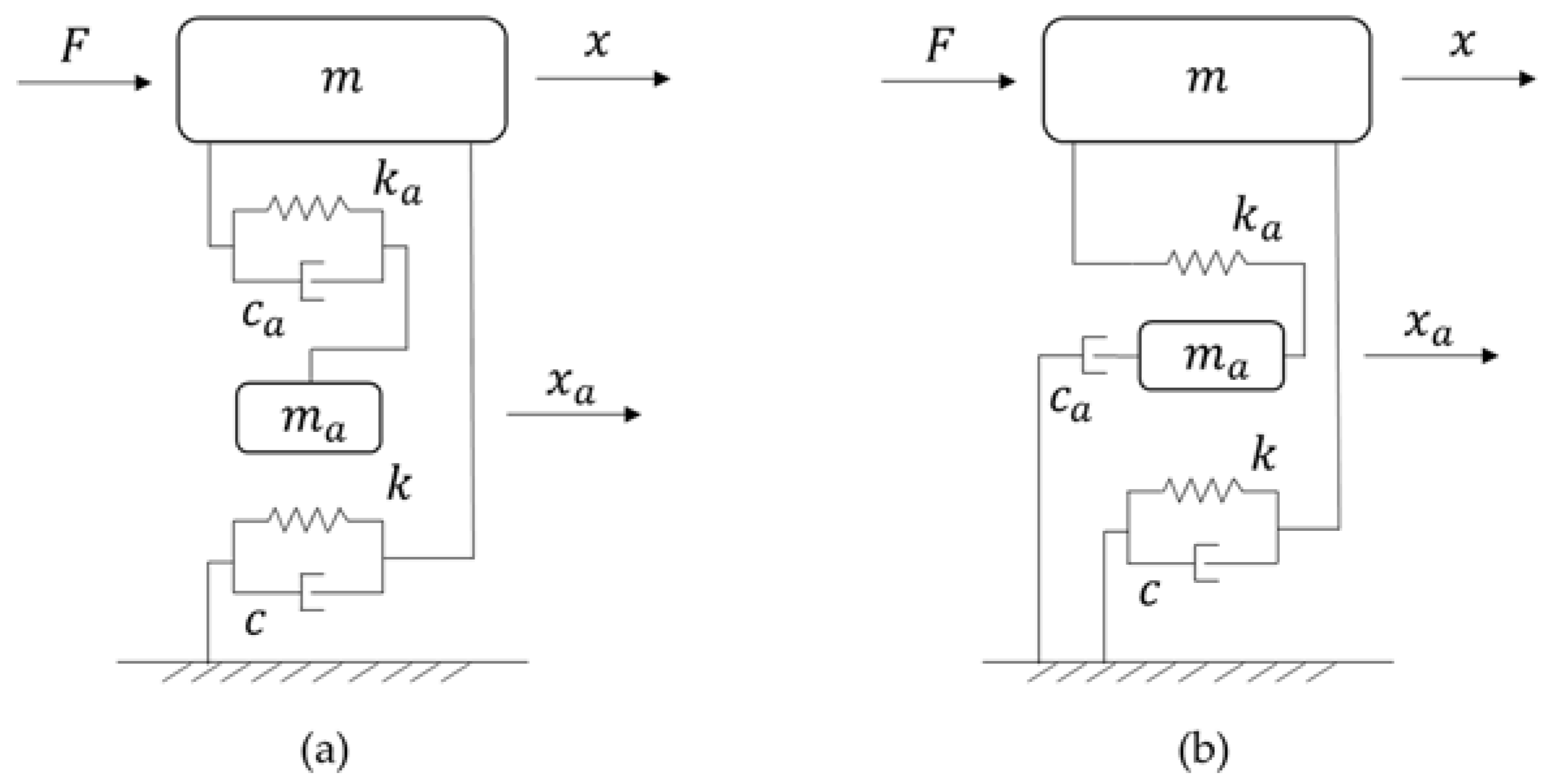
Vibration absorber or tuned mass damper (TMD) consists of mass and spring. When a host system is subjected to a harmonic excitation, its steady state response can be suppressed by using the vibration absorber with its natural frequency tuned to be the exciting frequency. The main shortcoming of the vibration absorber is a narrow operating bandwidth as its performance deteriorates significantly when the exciting frequency varies. Adding a damper in parallel with the absorber spring results in a damped vibration absorber. By designing the absorber damper properly, the operating bandwidth can be widened while the performance at the tuning frequency is compromised. Figure 1 shows two possible ways to add a damper. Model A is a traditional way and model B is a nontraditional way. The theories and methods to design an optimum damped model A are well developed [1,2,3,4]. Model B is considered to offer some advantages over model A. For example, when the damper requires a certain stroke space in a tight space, implementation of model B is easier than that of model A. For a pendulum-type TMD, model B may be the only viable option. When a vibration absorber is used to control resonance of a vibration isolator, placing the damper between the absorber mass and base reduces the amount of added mass to the isolated system. In [5], the optimum parameters of model B were investigated based on the “fixed-point” theory proposed in [1]. The study shows that given the same mass ratio, model B could offer more effective vibration control than model A. The results presented in [5] were verified by a slightly different approach in [6]. The use of model B to suppress vibration of a structure subjected to a harmonic ground excitation was addressed in [7]. The study reported in [8] addressed H2 optimization of model B for vibration control of structures under random excitation. The optimum parameters of model B in terms of minimizing the maximum velocity response were derived in [9]. The studies presented in [10,11] extended the optimum design of model B to a damped primary system. A detailed summary about the results of the optimum model B can be found in [12].

The interests of harvesting energy from ambient vibration have been driven by various applications such as power supply for wireless sensor networks [13], low-power actuators [14], and microsystems [15], etc. A typical vibration-based energy harvester consists of a mechanical system and a transduction device. The mechanical system couples environmental vibration to the transduction device that converts mechanical energy into electric one. A mass-spring system is a typical choice to maximize motion coupling. Three main transduction mechanisms are piezoelectric, electromagnetic and electrostatic. Many studies have been conducted on energy harvesting using the piezoelectricity [16,17,18,19,20,21,22]. Most of these studies have been focused on the following areas: the fundamental properties and modelling of piezoelectric material, the performance of piezoelectric devices under different external excitations, and the optimization of the harvested power. Similarly, a great amount of research has been conducted for another commonly used energy harvesting technique of using electromagnetic transduction [23,24,25,26,27,28,29].

Because a vibration-based energy harvester is similar to a vibration absorber, it is naturally desired to use the same device for simultaneous vibration suppression and energy harvesting. The dual mass system proposed in [30] consisted of a primary system and a vibration absorber. The system was utilized for energy harvesting from random force and base excitation. In [31], simultaneous vibration mitigation and energy harvesting were achieved by an electricity-generating tuned mass damper. A survey of control strategies for simultaneous vibration suppression and energy harvesting via piezoceramics was presented in [32]. The study presented in [33] integrated the tuned mass damper and electromagnetic shunted resonant damping to achieve a dual functional energy harvesting and vibration control. However, it should be noted that the existing attempts for the aforementioned purpose use model A. In [34], a model B based apparatus was developed for vibration suppression and energy harvesting. It is comprised of a primary system and a tunable model B. Both the stiffness and damping of the developed model B can be tuned such that its optimum performance can be investigated. In [34] steady-state responses of the combined system under harmonic base excitation were considered in terms of vibration suppression and energy harvesting.

Although most of energy harvesters are designed to operate at a steady-state condition, their performances under time-limited or transient responses are also of interest. For example, various environmental vibrations are time-limited. In [35], energy harvesting in bridge systems was investigated. A cantilever beam applied with a piezoelectric patch was used as the energy harvester. The study considered both the forced vibration during the vehicle passing and the free vibration after the vehicle passing. In [36], harvesting energy from the vibration of a passing train was investigated. The duration of the induced vibration depends on the speed of train and number of passenger coaches. The study focused on the maximum available energy that could be potentially harvested. Base excitation may be a series of impulses. In such a case, energy must be harvested from transient responses. In [37], an impact energy harvester was developed for the use in impulsive base excitation. The device consisted of two piezoelectric cantilever beams that are subjected impact of a sliding mass. The study dealt with both the transient responses and steady-state responses. Human motion is another example of shock excitation. In [38], two inductive energy harvesters were developed by exploiting different characteristics of the human gait. The first one is a multi-coil topology harvester that is aimed at the swing motion of the foot while the second one is a shock-type harvester that responds to heel strike. Transient responses provide an easy and quick way to test performance of a system. In [31], the proposed tuned mass damper was tested using free responses in order to demonstrate its effectiveness for vibration control and energy harvesting. The transient stage of an energy harvester is also an interesting aspect that has been investigated by some researchers. The study reported in [39] focused on the transient performance of energy harvesting systems initially at rest both mechanically and electrically. The standard and nonlinear harvesting circuits were compared in terms of harvested energy or time of harvesting. Transient behaviors of nonlinear energy harvesters become more intriguing and interesting. Especially nonlinear energy sink (NES) has been receiving increasing attention for its unique transient behaviors such as targeted energy transfer. Some attempts have been made to use the NES or its variant form for simultaneous vibration suppression and energy harvesting [40,41,42]. This paper investigates transient performance of the apparatus developed in [34].

The rest of the paper is organized as follows. Section 2 introduces the developed apparatus. Section 3 discusses the design of optimum model B for suppression of transient responses. Section 4 defines an index to measure the performance of energy harvesting. Section 5 presents a computer simulation study. Section 6 reports an experimental validation. Section 7 draws the main conclusions of the study.

2. Apparatus

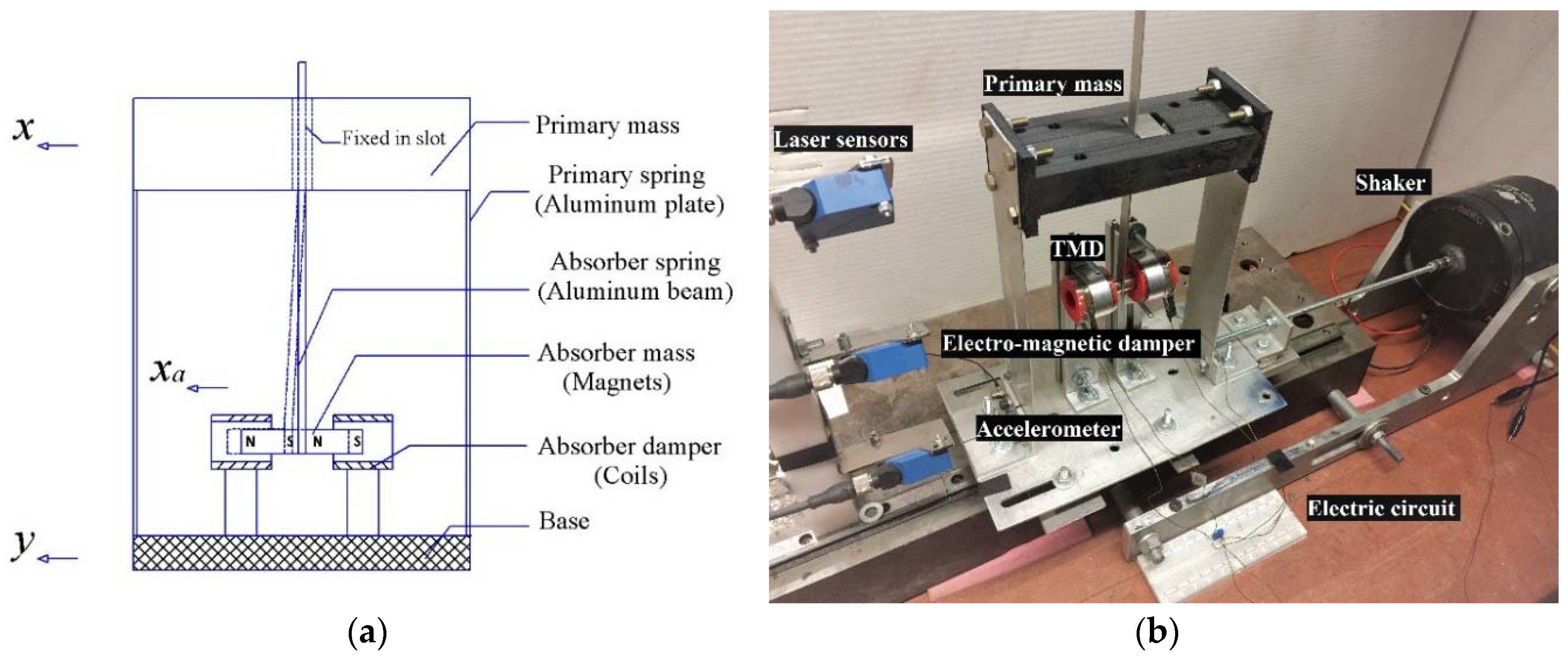
Figure 2a shows the schematic of the apparatus used in this study. Figure 2b shows a photo of the experimental set-up. The primary system consists of a 3-D print platform used as the primary mass and two aluminum plates used as the primary spring. The primary system is clamped to a base plate that is fastened to the ground in this study. A tunable vibration absorber is constructed by an aluminum beam that acts as a spring and a pair of magnets that act as a mass. The dimensions of the beam and magnets can be found in [34]. The upper end of the beam is clamped in a slot built in the primary mass block. By sliding the beam in the slot, its length can be adjusted so that the absorber’s natural frequency can be varied. A pair of coils are fastened on aluminum extrusions that are fixed on the base plate. As shown in Figure 2a, the two magnets are partially situated inside the coils to form an electromagnetic energy harvester. An electric circuit is formed by connecting the coils in series with a variable resistor that serves as an energy harvesting load.

Table 1. Parameters of the coils.

Inner Radius (mm)	Outer Radius (mm)	Length (mm)	Turns	Coil resistance (Ω)
12.175	18.525	31.75	320	2.3

lists the parameter values for the magnets and coils. Comparing Figure 2a with Figure 1b reveals that the developed apparatus belongs to model B because the absorber damper is connected between the absorber mass and the ground.

3. Optimum Model B for Suppression of Transient Responses

An optimum criterion is needed in order to design an optimum Model B. In [12], the stability maximization criterion (SMC) was employed for this purpose. The SMC is briefly outlined below. The state-space model of a linear system of an order $N$ with a single input can be given by

$$\dot{\mathit{X}}=\mathit{A}\mathit{X}+\mathit{B}\mathit{u}$$

(1)

where $\mathit{X}$ and $\mathit{u}$ are the state vector and input, respectively, $\mathit{A}$ is the state matrix and $\mathit{B}$ is the input influence vector. If all the eigenvalues ${\lambda }_i(i=1,2,\cdots ,N)$ of the state matrix is distinctive, $\mathit{A}$ is diagonalizable and semi-simple. Then the free response of the system can be written as

$$\mathit{X}(t)=e^{A(t-t_0)}\mathit{X}(t_0)={\displaystyle \sum _{i=1}^N{\mathit{P}}_i\mathit{X}(t_0)e^{{\lambda }_i(t-t_0)}}$$

(2)

where $\mathit{X}(t_0)$ is the initial state vector and ${\mathit{P}}_i$ is a matrix that can be found by the Lagrange’s interpolation polynomial as

$${\mathit{P}}_i=\frac{(\mathit{A}-{\lambda }_1\mathit{I})\cdots (\mathit{A}-{\lambda }_{i-1}\mathit{I})(\mathit{A}-{\lambda }_i\mathit{I})\cdots (\mathit{A}-{\lambda }_N\mathit{I})}{({\lambda }_i-{\lambda }_1)\cdots ({\lambda }_i-{\lambda }_{i-1})({\lambda }_i-{\lambda }_{i+1})\cdots ({\lambda }_i-{\lambda }_N)}$$

(3)

where $\mathit{I}$ is an unit matrix. The degree of stability of the system is defined as the absolute value of the maximum real part of the eigenvalues,

$$\mathsf{\Lambda }=\underset{i}{-\max }\mathrm{Re}({\lambda }_i)$$

(4)

Apparently the variable $\mathsf{\Lambda }$ represents the slowest decaying speed of the modal response. The following inequality holds:

$$\left|\mathit{X}(t)\right|=\left|e^{A(t-t_0)}\mathit{X}(t_0)\right|\le {\displaystyle \sum _{i=1}^N\left|{\mathit{P}}_i\mathit{X}(t_0)\right|e^{\mathsf{\Lambda }(t-t_0)}}$$

(5)

By maximizing $\mathsf{\Lambda }$, all the eigenvalues are forced to move far away from the imaginary axis in the left-hand complex plane so that the fastest decaying response can be achieved.

In what follows, application of the SMC to model B is briefly introduced. The equations of motion for free responses of the combined system can be defined by

$$m\ddot{x}+(k+k_a)x-k_a{x}_a+c\dot{x}=0$$

(6)

$$m_a{\ddot{x}}_a+c_a{\dot{x}}_a+k_a{x}_a-k_{a}x=0$$

(7)

where $m$ and $m_a$ are the mass of the primary system and the absorber system, respectively, $k$ and $k_a$ are the stiffness of the primary system and absorber system, respectively, $c$ and $c_a$ are the damping coefficient of the primary system and absorber system, respectively, $x$ and $x_a$ are the displacement of the primary system and absorber system, respectively. To facilitate analysis, Equations (6) and (7) can be reformulated as

$$\ddot{x}+({\omega }_p^2+\mu {\omega }_a^2)x-\mu {\omega }_a^2{x}_a+2{\zeta }_p{\omega }_p\dot{x}=0$$

(8)

$${\ddot{x}}_a+2{\zeta }_a{\omega }_a{\dot{x}}_a+{\omega }_a^2{x}_a-{\omega }_a^{2}x=0$$

(9)

by introducing the following variables

$${\omega }_p=\sqrt{\frac{k}{m}},{\omega }_a=\sqrt{\frac{k_a}{m_a}},\mu =\frac{m_a}{m_p},\beta =\frac{{\omega }_a}{{\omega }_p},{\zeta }_p=\frac{c}{2m_a{\omega }_p},{\zeta }_a=\frac{c_a}{2m_a{\omega }_a}$$

where ${\omega }_p$ and ${\omega }_a$ are the natural frequency of the primary system and absorber system, respectively, ${\zeta }_p$ and ${\zeta }_a$ are the damping ratio of the primary system and absorber system, respectively, $\mu$ is referred to as the mass ratio, and $\beta$ is referred to as the frequency tuning ratio. A dimensionless time $\tau ={\omega }_{p}t$ is defined so that the following relationships hold

$$\ddot{x}=\frac{d^{2}x}{d{t}^2}={\omega }_p^2\frac{d^{2}x}{d{\tau }^2}={\omega }_p^2{x}^{″},\dot{x}=\frac{dx}{dt}={\omega }_p\frac{dx}{d\tau }={\omega }_p{x}^{\prime }$$

(10)

Then Equations (8) and (9) become

$$x^{″}+(1+\mu {\beta }^2)x-\mu {\beta }^2{x}_a+2{\zeta }_p\dot{x}=0$$

(11)

$${x^{″}}_a+2\beta {\zeta }_a{\dot{x}}_a+{\beta }^2{x}_a-{\beta }^{2}x=0$$

(12)

With $\mathit{X}={[x^{\prime },{x^{\prime }}_a,x,x_a]}^T$, the state matrix $\mathit{A}$ can be expressed as

$$\mathit{A}=\left[\begin{array}{cccc}-2{\zeta }_p& 0& -(1+\mu {\beta }^2)& \mu {\beta }^2\\ 0& -2\beta {\zeta }_a& {\beta }^2& -{\beta }^2\\ 1& 0& 0& 0\\ 0& 1& 0& 0\end{array}\right]$$

(13)

The characteristic equation of the system is given as

$${\lambda }^4+2(g+{\zeta }_p){\lambda }^3+({\beta }^2+4{\zeta }_{p}g+1+\mu {\beta }^2){\lambda }^2+2({\zeta }_p{\beta }^2+g+\mu g{\beta }^2)\lambda +{\beta }^2=0$$

(14)

where $g=\beta {\zeta }_a$. For the system under consideration, the eigenvalues or the roots of Equation (14) are two pairs of complex conjugates that can be denoted as ${\lambda }_{1,2}=-a_1\pm j{b}_1,{\lambda }_{3,4}=-a_2\pm j{b}_2$. Then Equation (14) can be recast as

$$(\lambda +a_1+j{b}_1)(\lambda +a_1-j{b}_1)(\lambda +a_2+j{b}_2)(\lambda +a_2-j{b}_2)=0$$

(15)

Comparing the coefficients of Equation (15) with their counterparts of Equation (14) yields

$$2(g+{\zeta }_p)=2(a_1+a_2)$$

(16)

$${\beta }^2+4{\zeta }_{p}g+1+\mu {\beta }^2=s_1^2+s_2^2+4a_1{a}_2$$

(17)

$$2({\zeta }_p{\beta }^2+g+\mu g{\beta }^2)=2(a_1{s}_1^2+a_2{s}_2^2)$$

(18)

$${\beta }^2=s_1^2{s}_2^2$$

(19)

where $s_1^2=a_1^2+b_1^2$ and $s_2^2=a_2^2+b_2^2$. The derivation presented in [12] shows that the degree of stability will be maximized if the following conditions are satisfied:

$$a_1=a_2,s_1=s_2$$

(20)

If the primary system is free of damping or ${\zeta }_p=0$, the optimum frequency tuning ratio is found to be

$${\beta }^{*}=\frac{1-\sqrt{1-4\mu }}{2\mu }$$

(21)

And optimum damping ratio is given by

$${\zeta }_a^{*}=\frac{\sqrt{1-\sqrt{1-4\mu }}}{\sqrt{2}}$$

(22)

4. Index to Measure the Performance of Energy Harvesting

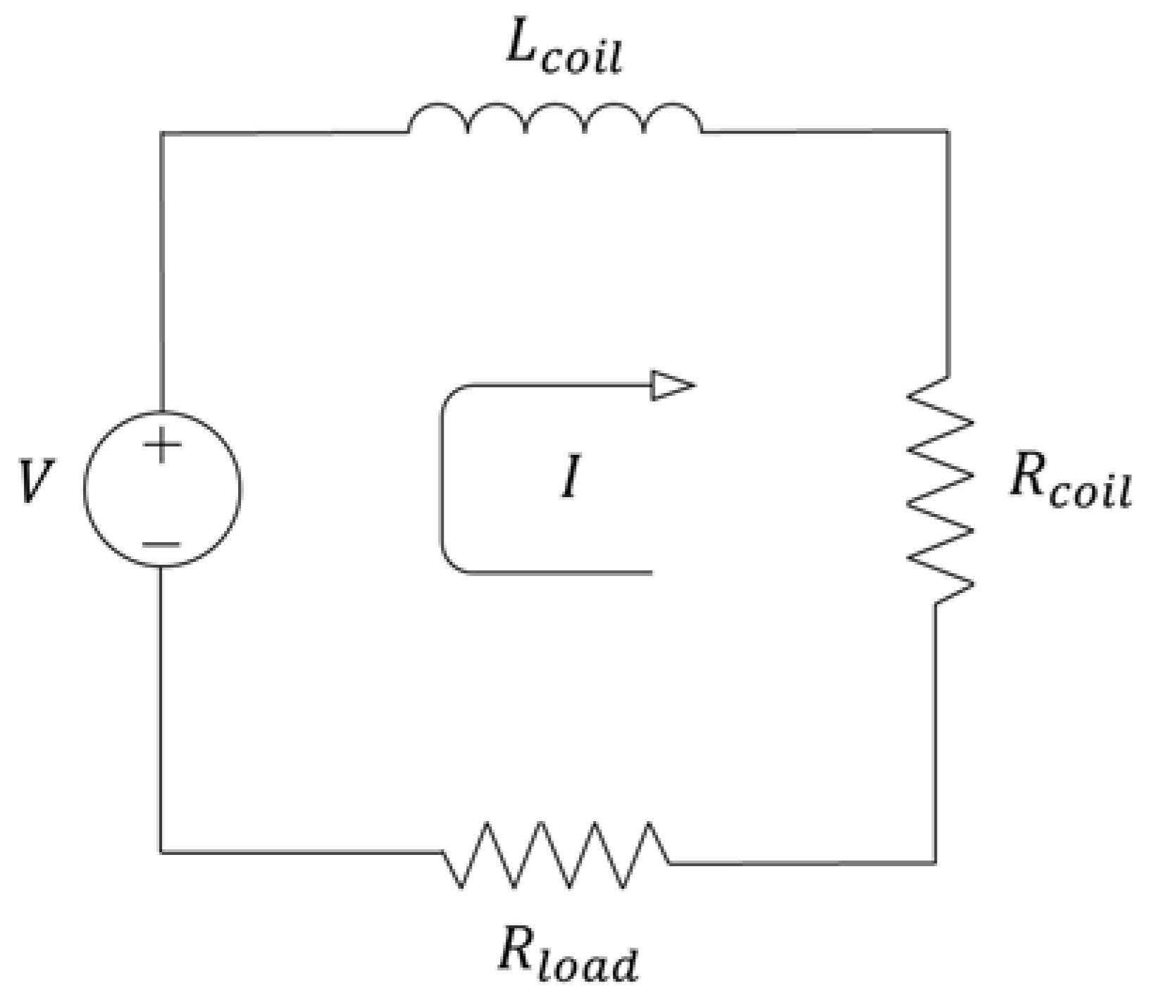
An index is needed to measure the performance of energy harvesting. In order to compute the harvested energy, the electro-mechanical coupling between the energy harvesting circuit and the absorber motion is briefly introduced. Figure 3 shows the circuit of energy harvesting for one coil where $L_{coil}$ and $R_{coil}$ are the inductance and resistance of the coil, respectively, and $R_{load}$ is the resistance of a resistive load. When the two coils are connected in series, applying Kirchhoff’s law to the circuit yields

$$2L_{coil}\frac{di}{dt}+\left(2R_{coil}+R_{load}\right)i=\mathsf{\Theta }{\dot{x}}_a$$

(23)

where $i$ is the induced current in the coils, $\mathsf{\Theta }$ is the so-called total transduction factor for the two coils connected in series, and ${\dot{x}}_a$ is the velocity of the absorber mass (magnets) relative to the base that is stationary for the case of free responses. The inductance’s effect can be neglected as its value is very small and frequency under consideration is low [34]. Thus the current can be approximated by

$$i=\frac{\mathsf{\Theta }}{2R_{coil}+R_{load}}{\dot{x}}_a$$

(24)

On the other hand, when the magnets are moving inside the coils, an electro-magnetic force is induced to oppose the motion. The electro-magnetic force $F_e$ is given by [34]

$$F_e=\mathsf{\Theta }i$$

(25)

Substituting Equation (24) in Equation (25) results in

$$F_e=c_e{\dot{x}}_a$$

(26)

where

$$c_e=\frac{{\mathsf{\Theta }}^2}{2R_{coil}+R_{load}}$$

(27)

is referred to as electrical damping coefficient.

For free response, the initial energy $E_{in}$ of the system is defined by

$$E_{in}=\frac{1}{2}k{X}_0^2+\frac{1}{2}m{V}_0^2+\frac{1}{2}{k}_a{(X_{a0}-X_0)}^2+\frac{1}{2}{m}_a{V}_{a0}^2$$

(28)

where $X_0$ and $X_{a0}$ are the initial displacement of the primary system and absorber system, respectively, $V_0$ and $V_{a0}$ are the initial velocity of the primary system and absorber system, respectively. The power harvested by the load resistor can be found by

$$p_{load}(t)=i^2(t)R_{load}=\frac{{\mathsf{\Theta }}^2{R}_{load}}{{(2R_{coil}+R_{load})}^2}{\dot{x}}_a^2(t)$$

(29)

Then the total harvested energy over a period $T$ can be computed by

$$E_{load}={\displaystyle {\int }_o^T{p}_{load}(t)dt}$$

(30)

An index that measures the performance of energy harvesting is defined as

$$I=\frac{E_{load}}{E_{in}}$$

(31)

When the primary system is damped, Equation (31) can also be written as

$$I=\frac{E_{load}}{E_{cm}+E_{ce}}$$

(32)

where $E_{cm}$ is the energy dissipated by the primary damper and $E_{ce}$ is the energy dissipated by the absorber damper. As the mechanical damping of the absorber system is negligible compared to the electrical damping induced by the energy harvesting system, the amount of the harvested energy satisfies,

$$E_{load}=\frac{R_{load}}{2R_{coil}+R_{load}}{E}_{ce}$$

(33)

5. Computer Simulation

A computer simulation is conducted to verify the optimum model B and investigate the energy harvesting efficiency. The parameter values used in the following simulation are based on the developed apparatus shown in Figure 2. For the primary system, $m=0.34$ kg and $k=2568.0$ N/m. For the absorber system, $m_a=0.048$ kg. The simulation considers both the undamped primary system and damped primary system.

5.1. Undamped Primary System

The optimum frequency tuning ratio and damping ratio for an undamped system are given by Equations (21) and (22). Using the mass ratio $\mu =m_a/m=0.048/0.34=0.141$, it is found that

$${\beta }^{*}=1.205,{\zeta }_a^{*}=0.4124$$

(34)

To verify the optimum parameters, a multi-objective optimization is conducted with two objective functions defined as

$$J_1(\beta ,{\zeta }_a)=\max (a_1,a_2)-\min (a_1,a_2)$$

(35)

$$J_2(\beta ,{\zeta }_a)=\left|\sqrt{a_1^2+b_1^2}-\sqrt{a_2^2+b_2^2}\right|$$

(36)

The first objective function measures the closeness of the real parts of the eigenvalues while the second objective function represents the closeness of the two natural frequencies of the combined system. A multi-objective optimization function in Matlab Global Optimization toolbox is used to search for the minimum objective functions within the range of $0\le \beta \le 1.5$ and $0\le {\zeta }_a\le 1$. This function uses the genetic algorithm to search for the solutions on the so-called Pareto front. A Pareto front is a set of nondominated solutions, being chosen as optimal, if no objective function can be improved without sacrificing at least one other objective function. All solutions in a Pareto set are equally optimal. The solution corresponding to the smallest damping ratio is chosen

$${\beta }^{*}=1.2048,{\zeta }_a^{*}=0.4122$$

(37)

with the corresponding objective function values as

$$J_1({\beta }^{*},{\zeta }_a^{*})=0.0001,J_2({\beta }^{*},{\zeta }_a^{*})=0.0352$$

(38)

These optimum values are almost identical to those given by the analytical results, verifying the correctness of Equations (21) and (22).

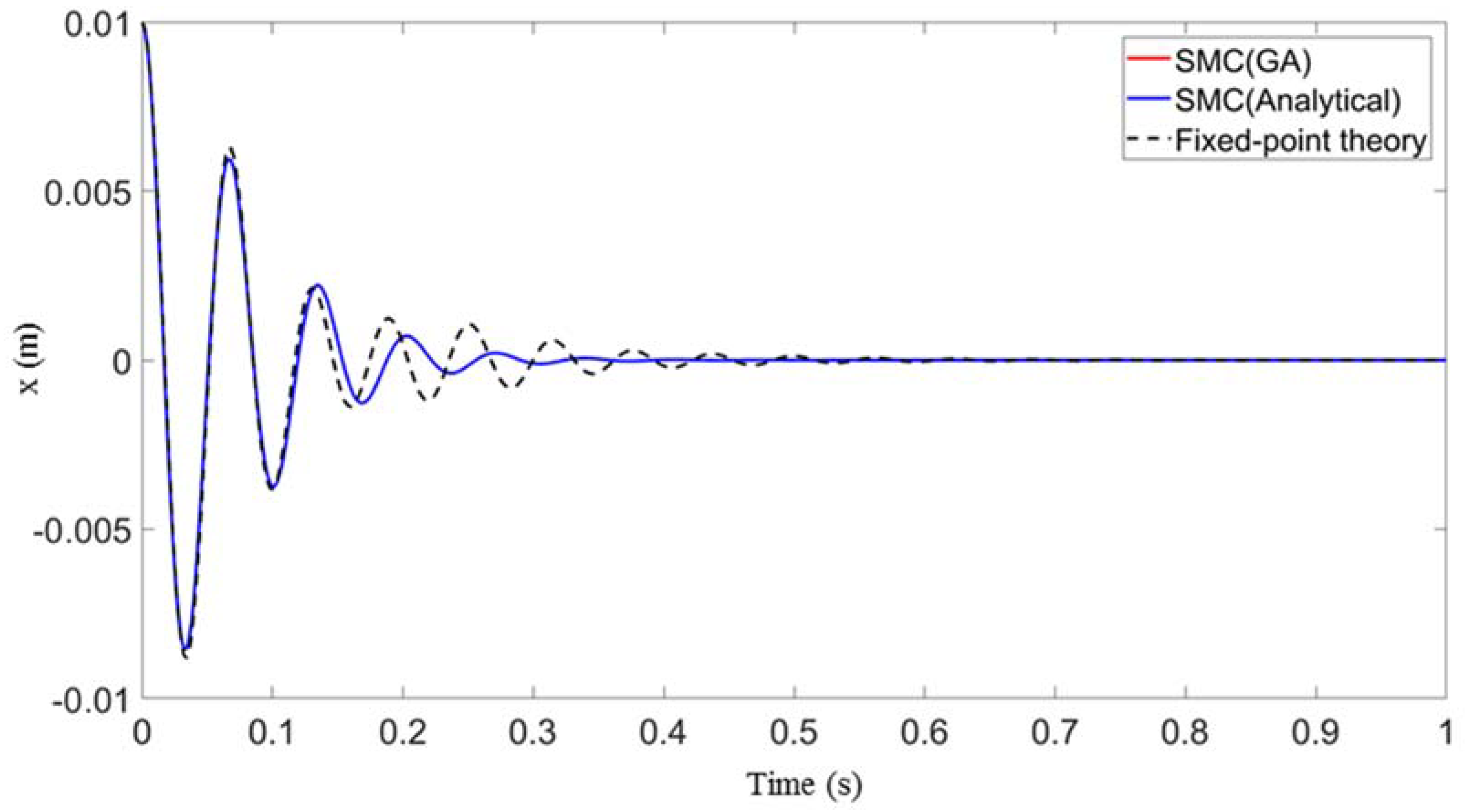
The transient responses of the system are generated with the initial conditions of $X_0=0.01$ m, $X_{a0}=0$, and $V_0=V_{a0}=0$. Figure 4 compares the responses of the primary mass from the system that is tuned in three different ways where SMC (GA) corresponds to the values given by Equation (37), SMC (Analytical) corresponds to the values given by Equation (34), and Fixed-points theory corresponds to the values determined by

$${\beta }^{*}=\sqrt{\frac{2}{2-\mu }}$$

(39)

and

$${\zeta }_a^{*}=\frac{1}{2}\sqrt{\frac{\mu \left({\mu }^2-8\mu -12\right)}{\left(\mu -2\right)\left({\mu }^2+2\mu +4\right)}}$$

(40)

The derivation of Equations (39) and (40) can be found in [34]. It can be seen that the first two responses are almost identical and decay faster than the third one. This reinforces the assertion that the fixed-point theory is not suitable for the case of suppressing the transient responses [12].

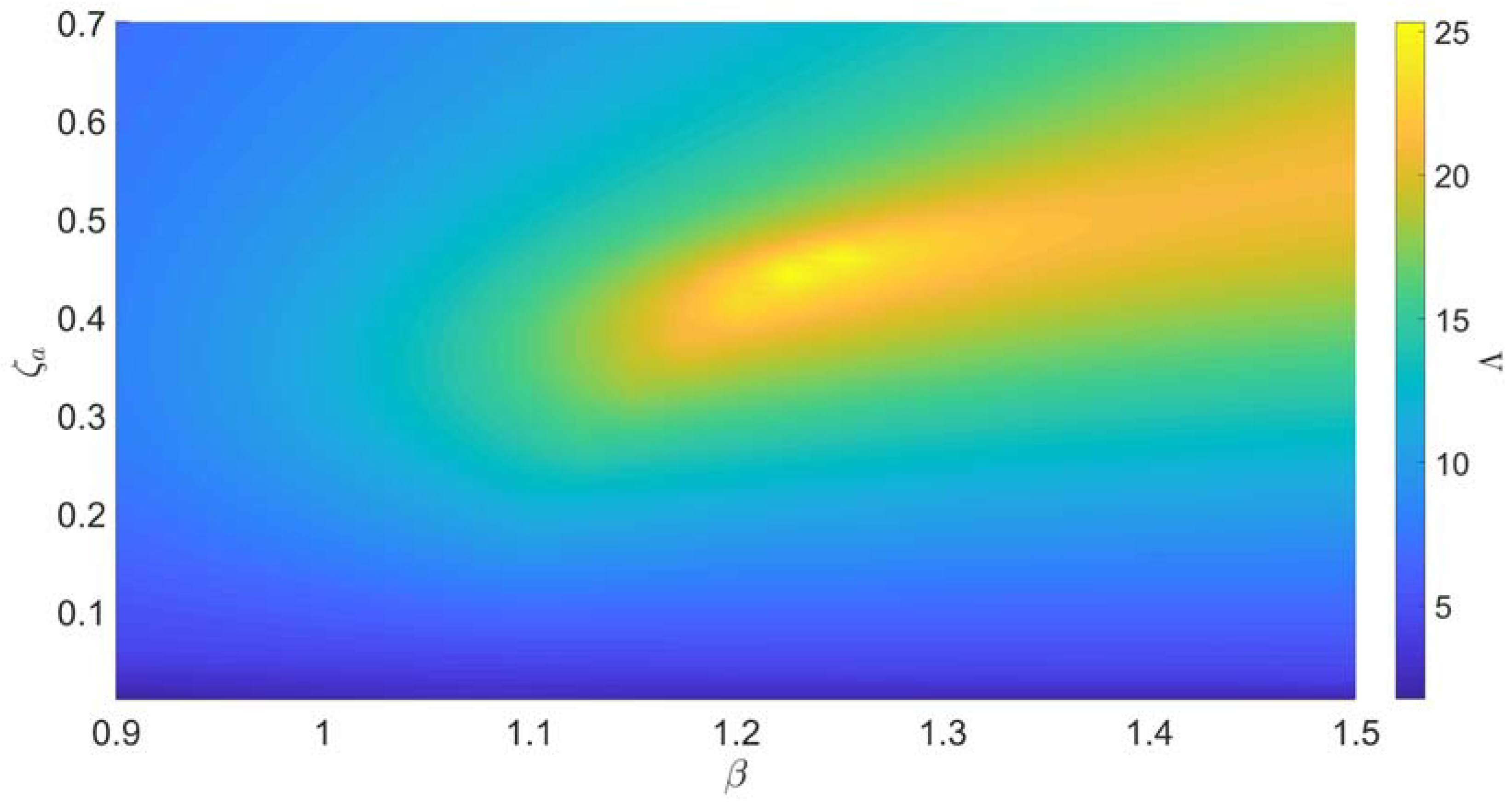
Simulations are also conducted to find out the relationship between the degree of stability and the tuning parameters. Figure 5 shows a contour plot of $\mathsf{\Lambda }$ vs. $\beta$ and ${\zeta }_a$. It can be seen that the maximum degree of stability occurs at the point of $\beta =1.2$ and ${\zeta }_a=0.41$. This is another validation for the analytical derivation. The plot also indicates that the greater the frequency tuning ratio, the higher the damping ratio is required to achieve a high degree of stability.

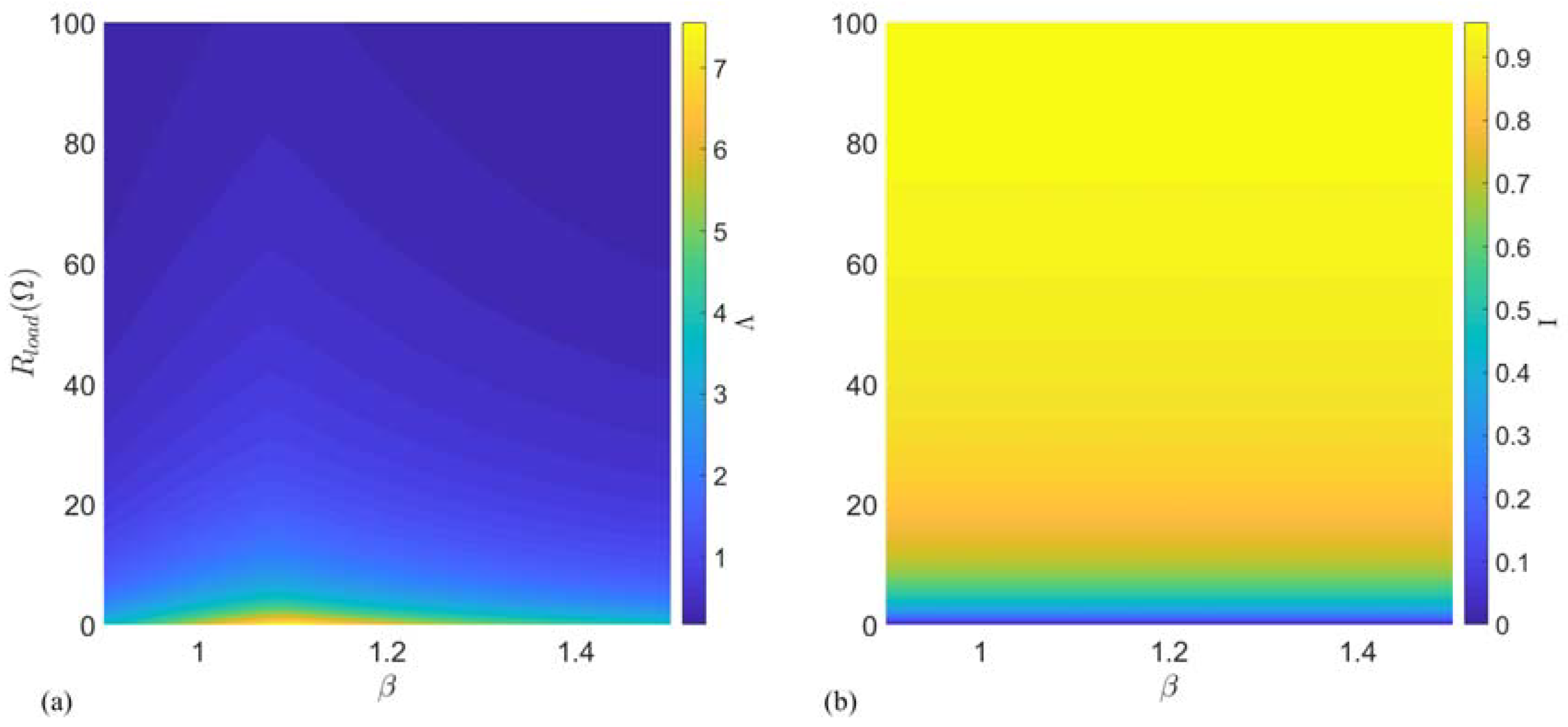
The mechanical damping in the absorber system is negligible compared with the electrical damping induced by the electromagnetic energy harvester [34]. To examine the effects of the load resistance $R_{load}$, it is assumed that $c_a=c_e$ or ${\zeta }_a={\zeta }_e$ in the following discussion. This way, the absorber damping coefficient is controlled by the load resistance defined by Equation (27). For the electromagnetic energy harvester used in the apparatus, the transduction factor is found to be $\mathsf{\Theta }=2.596$ Tm [34]. With the energy harvesting circuit is closed, the maximum damping coefficient is $c_{a\max }=1.465$ Ns/m, corresponding to the case of $R_{load}=0$. Thus, the maximum damping ratio is ${\zeta }_{a\max }=0.176$ if $\beta =1$. This means that the optimum damping ratio is not achievable by the present apparatus. Henceforth, the load resistance $R_{load}$ is treated as a tuning parameter. Figure 6a shows a contour plot for the degree of stability vs. $\beta$ and $R_{load}$. It can be seen that the highest degree of stability is achieved when $R_{load}=0$. It is easy to understand as the damping ratio is inversely proportional to the load resistance. Figure 6b shows the percentage of the harvested energy over the period of free responses. As predicted by Equation (32), the percentage of the harvested energy depends on only the load resistance if the primary system is undamped. The greater the load resistance, the greater the percentage of the harvested energy. This indicates that there is a trade-off between vibration suppression and energy harvesting.

5.2. Damped Primary System

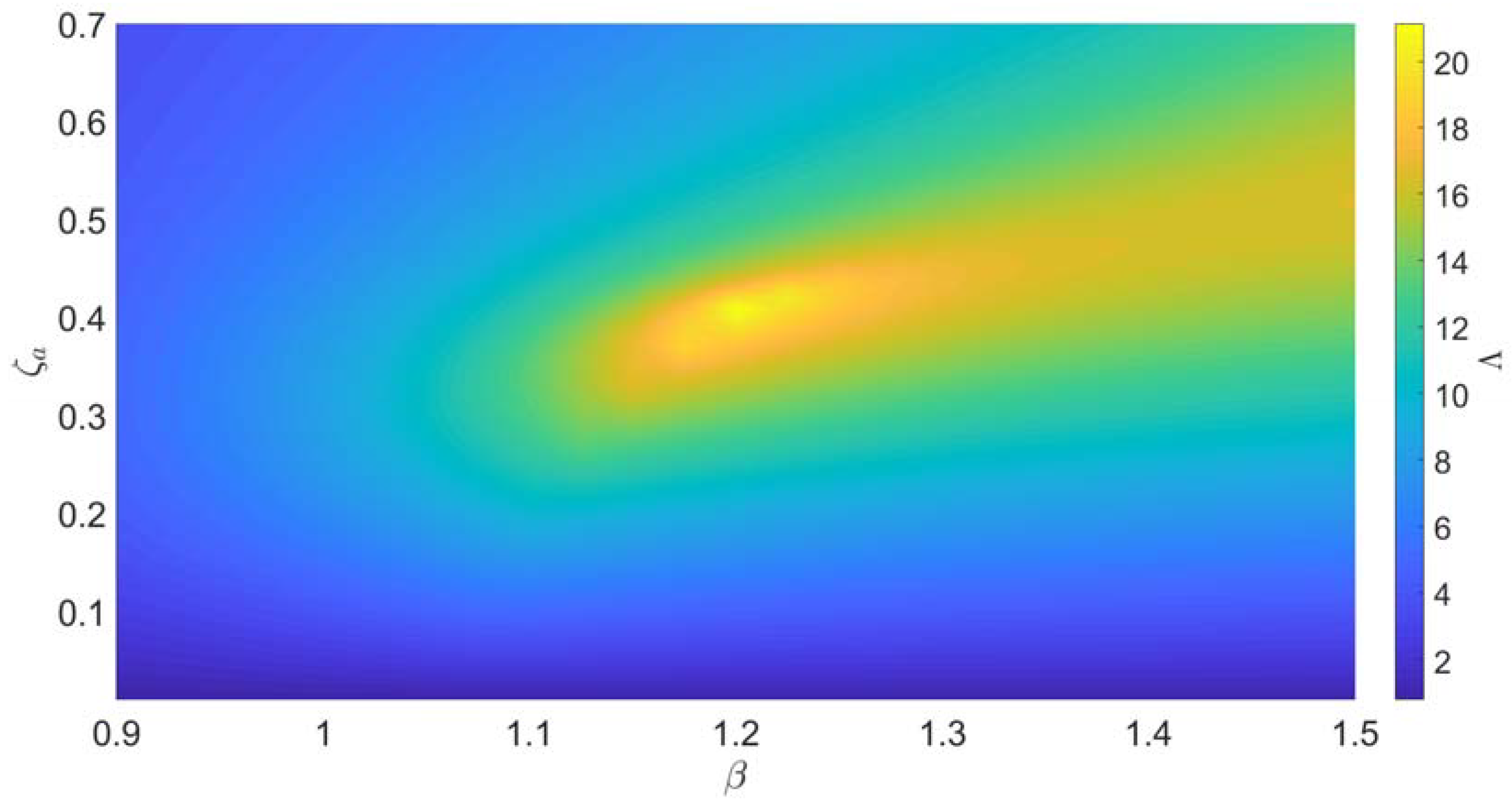
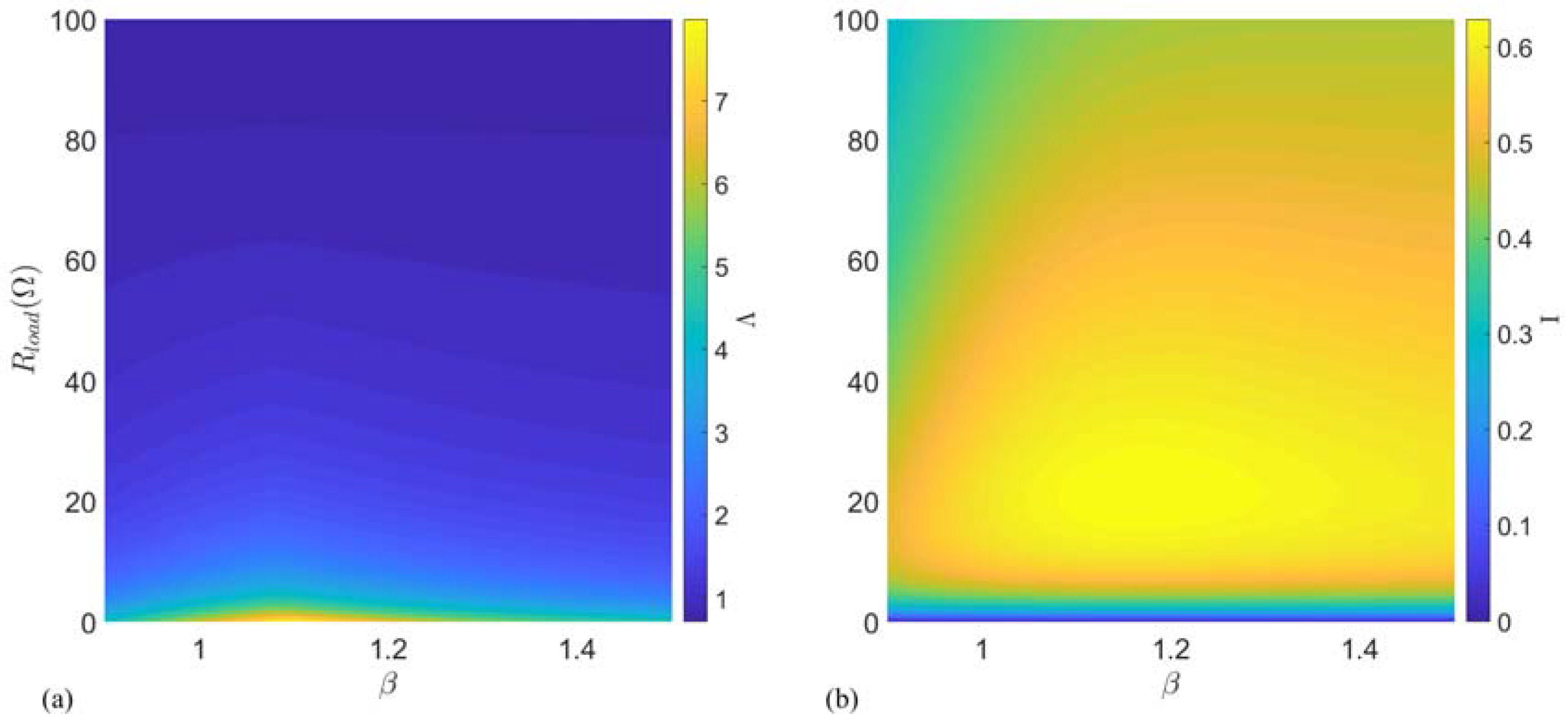
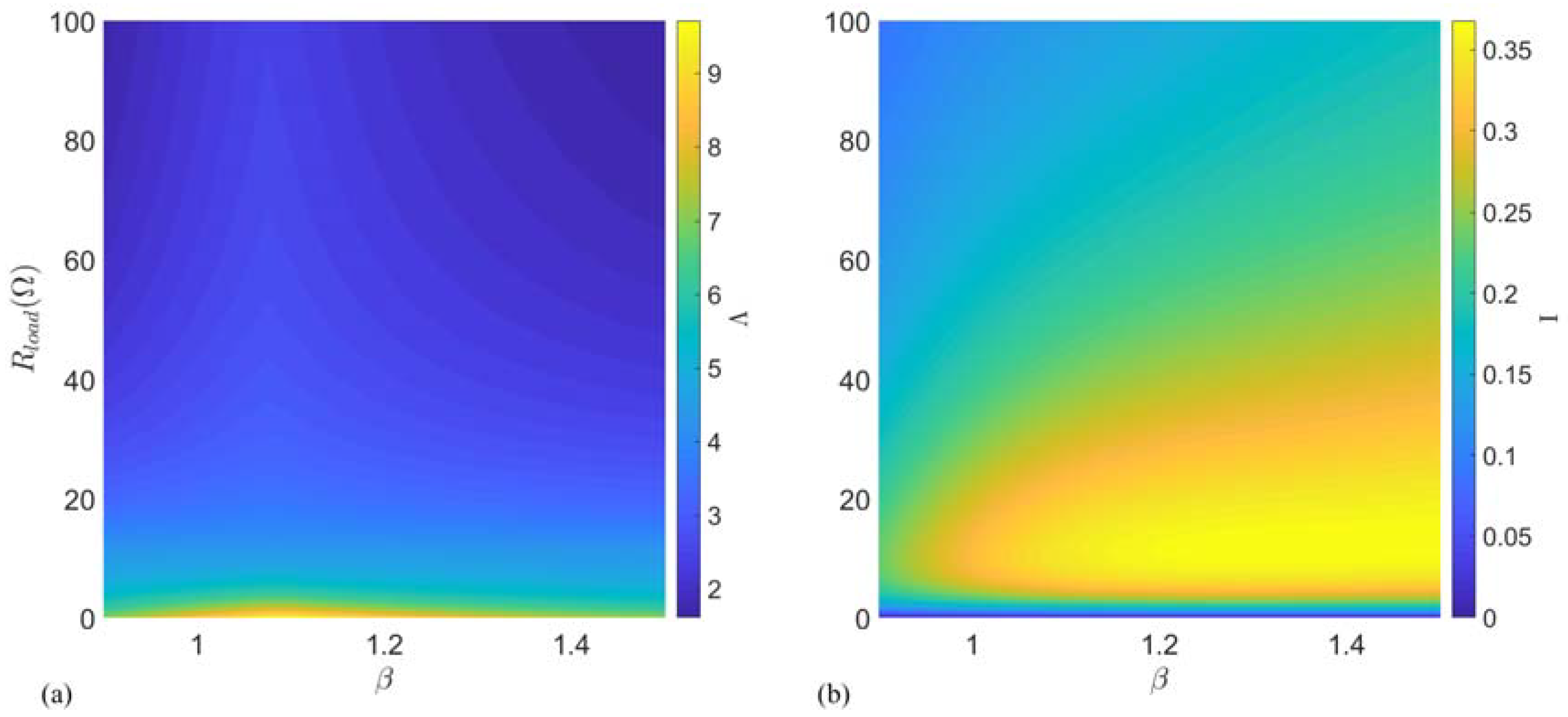
Now the effects of the primary damping are considered. Figure 7 shows the degree of stability vs. the frequency tuning ratio and damping ratio when $\zeta =0.01$. The maximum degree of stability still occurs at the point of $\beta =1.2$ and ${\zeta }_a=0.41$, indicating that a low level of damping in the primary system does not change the optimum parameters significantly. The degree of stability and the percentage of the harvested energy vs. the frequency tuning ratio and the load resistance are shown in Figure 8a,b, respectively. Again, from the viewpoint of vibration suppression, the load resistance should be set to zero. However, unlike the case of the undamped primary system shown in Figure 6b, there are the optimum load resistance and frequency tuning ratio that result in the maximum percentage of the harvested energy. This value is about $I_{\max }=0.63$ that occurs roughly at ${\beta }^{*}=1.175$ and $R_{load}^{*}=21\mathsf{\Omega }$ which corresponds to ${\zeta }_a^{*}=0.027$.

Figure 9 shows the case of increasing the primary damping ratio to 5%. With this damping level, there does not exist a maximum point within the parameter ranges under consideration. However, the general trend is that the maximum percentage of the harvested energy occurs around $R_{load}=12\mathsf{\Omega }$ when $\beta \ge 1.35$. For example, $I=0.3678$ at $\beta =1.35$ and $R_{load}=12\mathsf{\Omega }$ which corresponds to ${\zeta }_a=0.036$.

As shown in Figure 6, Figure 8, and Figure 9, there is a trade-off between the degree of stability and the harvested energy. To increase the system’s stability or suppress responses quickly, a zero load resistance is desired so that the absorber damping is maximized. However, depending on the level of the primary damping, there exists an optimum load resistance that maximizes the percentage of energy harvesting. To examine the trade-off situation, a multi-objective optimization is conducted. Two objective functions are defined as follows

$$J_1(\beta ,{\zeta }_a)=-\mathsf{\Lambda }$$

(41)

$$J_2(\beta ,{\zeta }_a)=-I$$

(42)

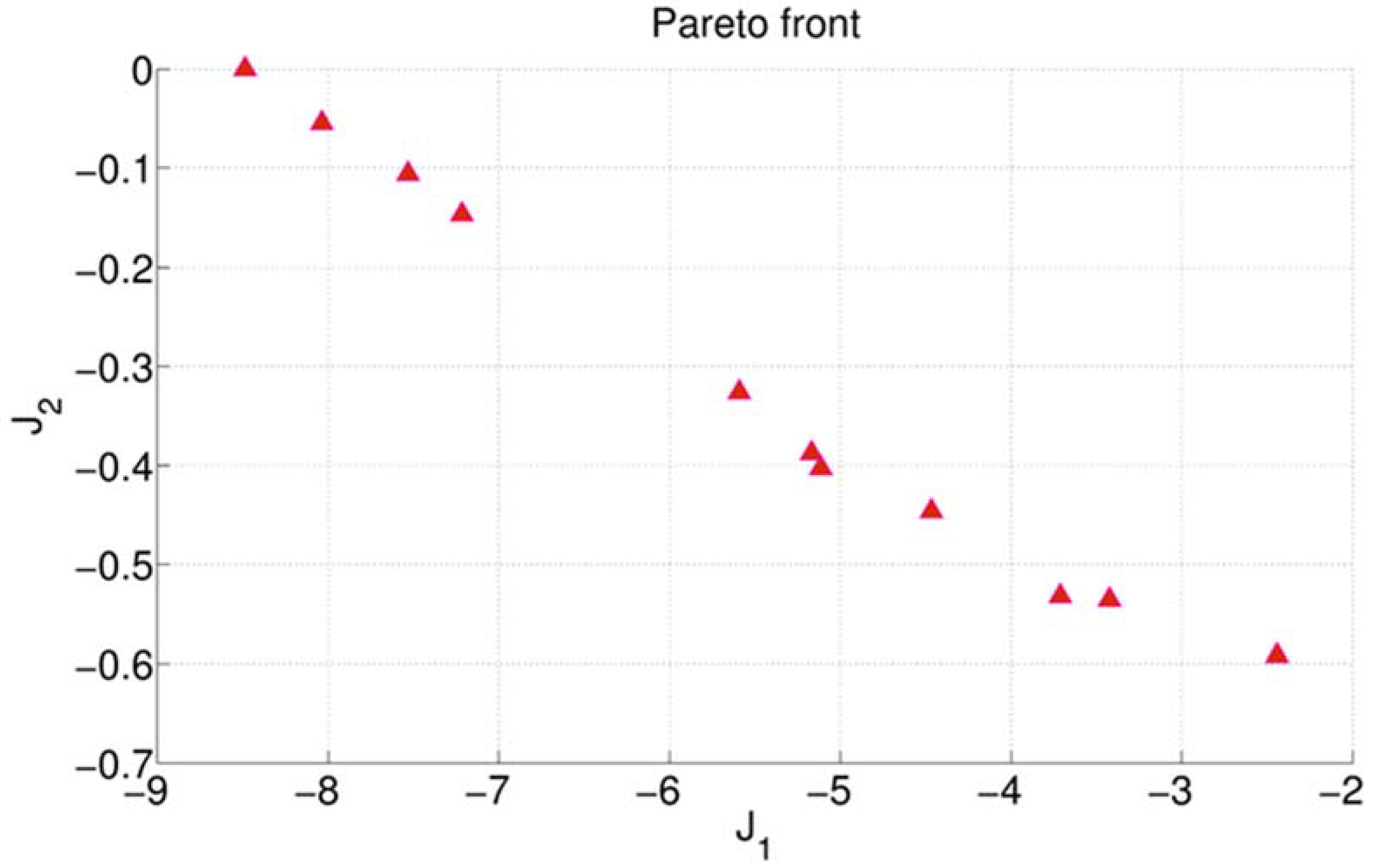
Again, a multi-objective optimization is conducted using the function built in Matlab Global Optimization toolbox to obtain the Pareto front. With the primary damping ratio of $\zeta =0.01$ and the search ranges of $0\le \beta \le 1.5$ and $0\le R_{load}\le 100\mathsf{\Omega }$, the obtained Pareto front is shown in Figure 10 and their corresponding values are listed in

Table 2. Solutions on the Pareto front.

$\mathit{\beta }$	${\mathit{R}}_{\mathit{l}\mathit{o}\mathit{a}\mathit{d}}(\mathsf{\Omega })$	$\mathit{I}$	$\mathsf{\Lambda }$
1.0986	0.0005	0.0001	8.4866
1.0989	0.2652	0.0548	8.0363
1.1043	0.7932	0.1471	7.2165
1.1050	0.5432	0.1061	7.5317
1.1052	3.3349	0.4027	5.1139
1.1147	6.2759	0.5323	3.7120
1.1236	2.2825	0.3261	5.5917
1.1437	3.0811	0.3876	5.1684
1.1461	3.9818	0.4463	4.4665
1.2110	6.0371	0.5357	3.4238
1.4863	7.0964	0.5919	2.4423

. It can be seen that the balanced choices for the $\beta$ and $R_{load}$ should be from the 5th row to 9th row in Table 2.

6. Experimental Results

An experimental study is conducted to verify the computer simulation results. A photo of the experimental set-up is shown in Figure 2b and the other details of the system can be found in [34]. By adjusting the length of the absorber beam, the frequency tuning ratio can be varied. A variable resistor is used to vary the load resistance from 0 to 100 $\mathsf{\Omega }$. Transient responses are generated by using the initial conditions: $X_0=X_{a0}=0.004$ m, and $V_0=V_{a0}=0$. The displacements of the primary mass and absorber mass are recorded by two laser reflex sensors (Wenglor CP24MHT80), respectively. The measured signals are preprocessed by a low-pass filter with a cut-off frequency of 80 Hz to reduce noise effect. The computer used in this study is equipped with a dSPACE dS1104 data acquisition board that collects the sensor signals and the voltage across the load resistor. A Simulink model is developed and connected to the dSPACE Control Desktop software to control the experiment. Using the measured voltage $V(t)$, the percentage of the harvested energy is calculated by

$$I=\frac{{\displaystyle {\int }_0^T{V}^2(t)/R_{load}dt}}{k{X}_0^2/2}$$

(43)

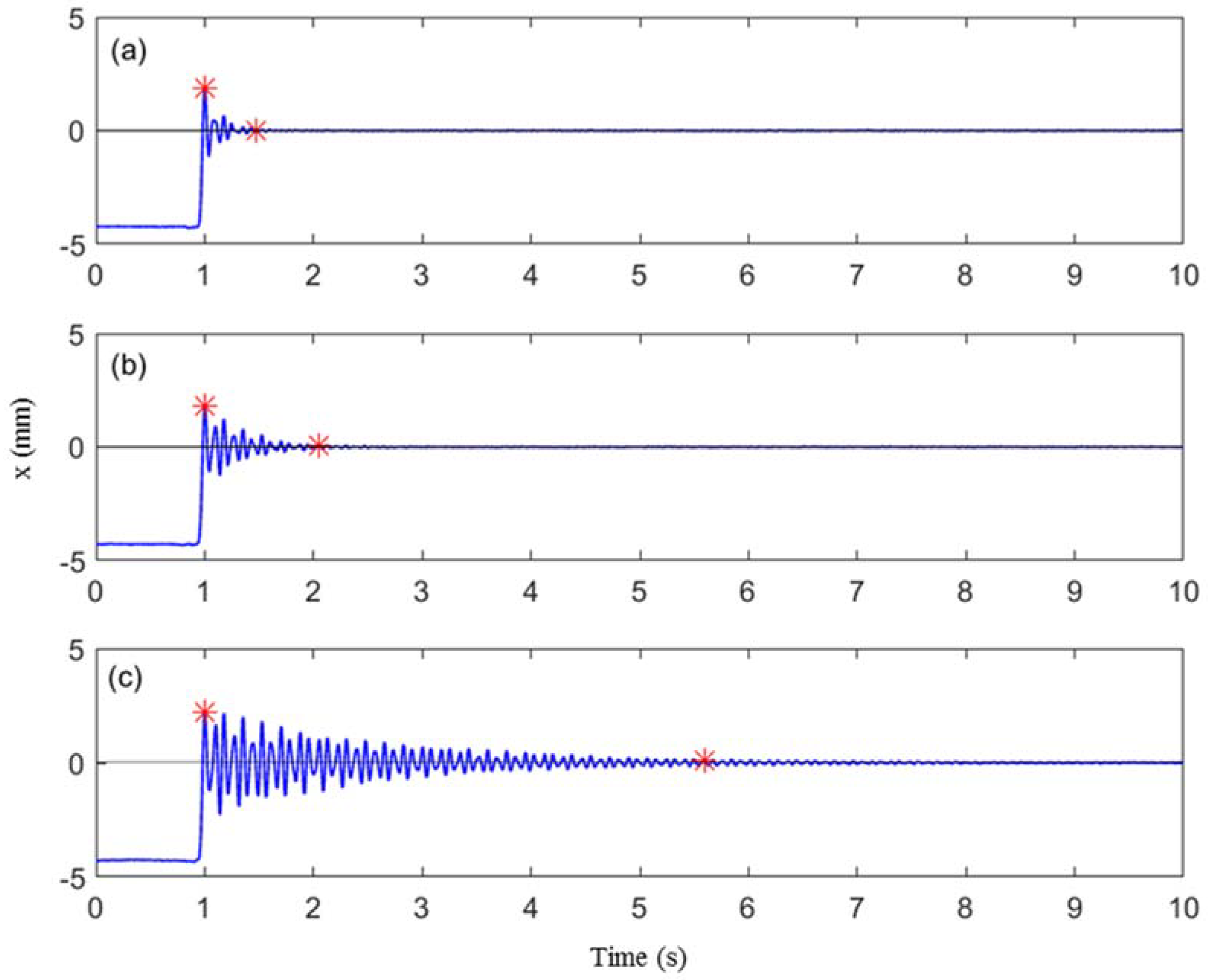
Figure 11 shows the responses of the primary mass when the load resistance takes three different values with the frequency tuning ratio set to be $\beta =1$. As shown in the figure, the smaller the load resistance, the faster the response decaying. The corresponding percentage of the harvested energy is also given in the figure. It is noted that these values are much smaller than those from the simulation. The explanation for such a discrepancy is that in the experiment, the primary mass is not able to oscillate back to the magnitude close to the initial displacement. This indicates that the real system is not exactly linear. Each of the responses in Figure 11 is marked by two asterisks. The first asterisk is placed at the highest peak while the second asterisk is placed at the first peak of those peaks that are equal or less than 5% of the highest peak. The duration $\mathsf{\Delta }t$ between the moment of the first asterisk and that of the second asterisk is referred to as the decaying time. The reciprocal of $\mathsf{\Delta }t$ or $1/\mathsf{\Delta }t$ is used as a measure for the degree of stability that is not readily available from the experimental results.

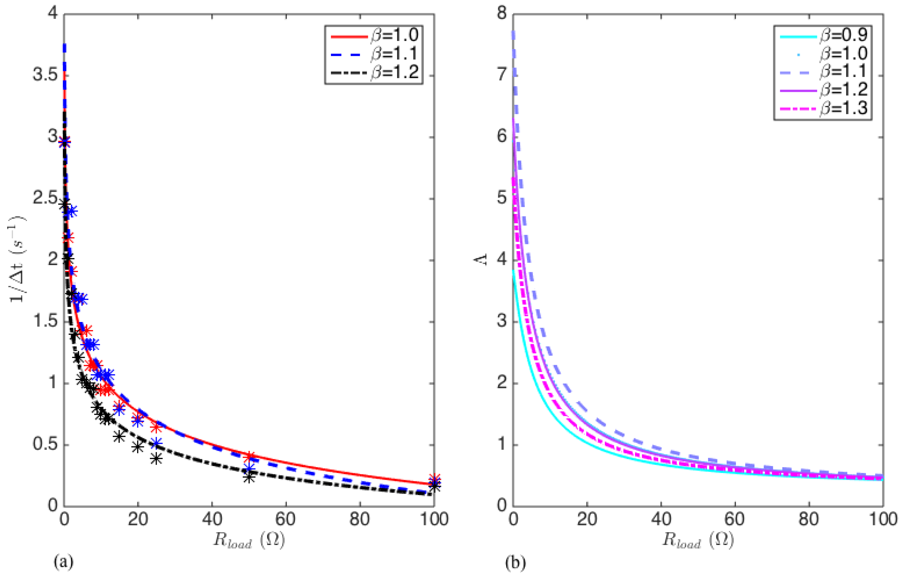
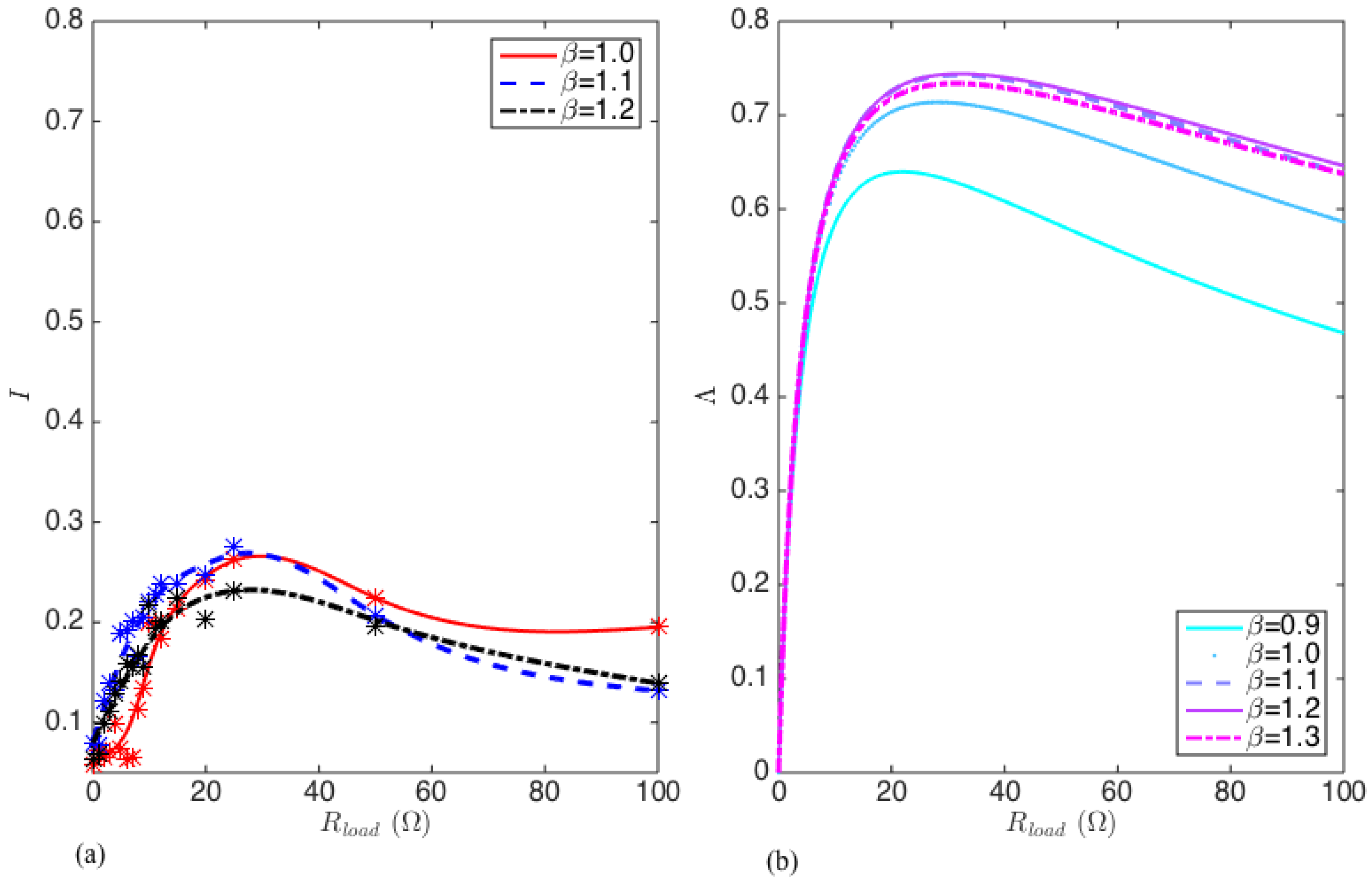
In what follows, the results obtained by three frequency tuning ratios $\beta =1.0,1.1,1.2$ are reported. For each of the three ratios, the load resistance $R_{load}$ is varied in the following sequence 0.2, 1, 2, 3, 4, 5, 6, 7, 8, 9, 10, 11, 12, 15, 20, 25, 50, 100 $\mathsf{\Omega }$. For each combination of $\beta$ and $R_{load}$, the measured response is used to find $\mathsf{\Delta }t$ and $I$. Figure 12a shows the reciprocals of the decaying times determined using the measured responses while Figure 12b shows the degree of stability determined using the simulation results. It can be seen that the general trends of $1/\mathsf{\Delta }t$ agree with those of $\beta$. The experimental results confirm that the degree of stability decreases with an increase of the load resistance. However, the influence of the frequency tuning ratio from the experimental results does not agree exactly with that from the simulation results.

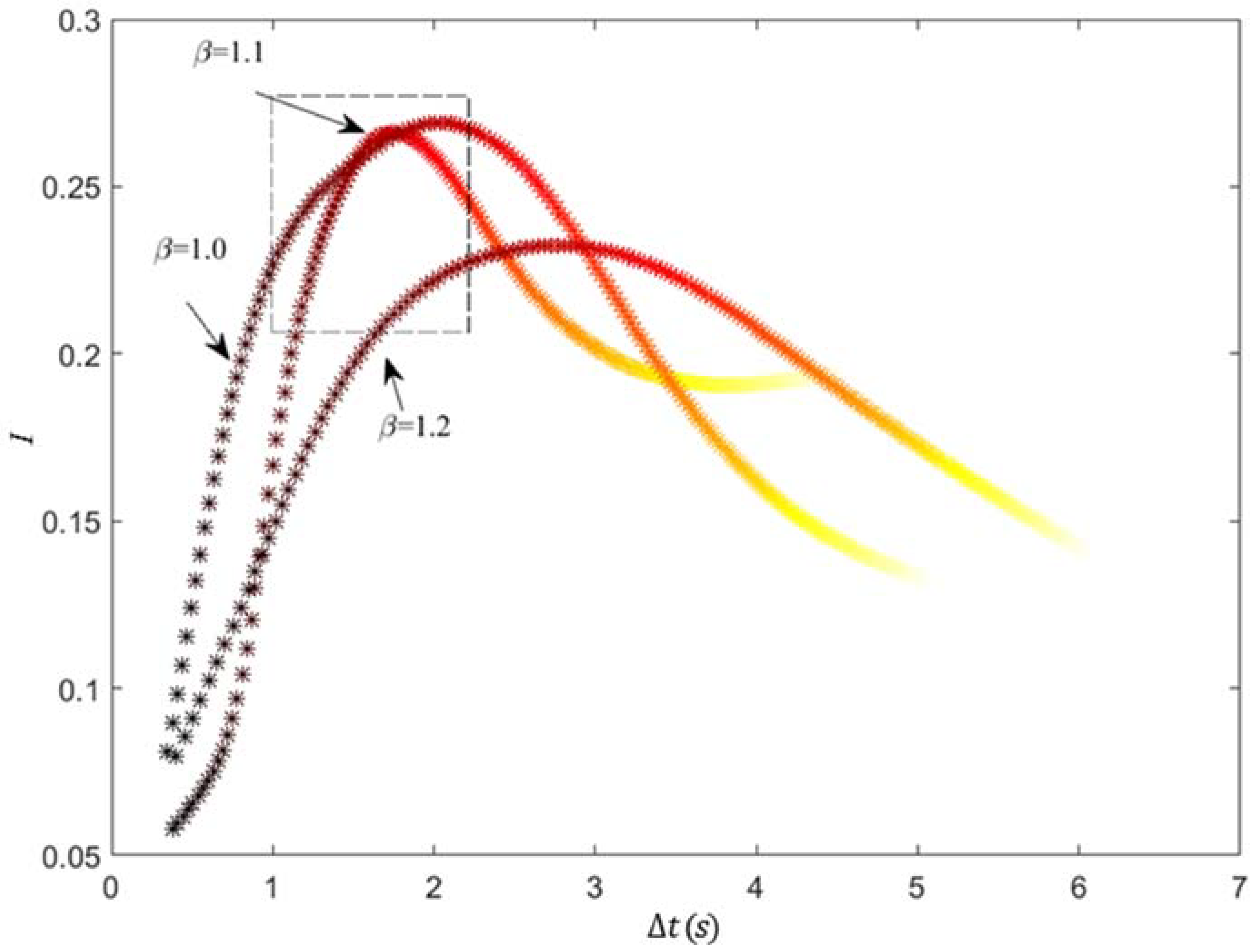
Figure 13a shows the percentages of the harvested energy based on the experimental results while Figure 13b gives the values based on the simulation results. It can be seen that the experimental results follow the general trends of the simulation results. For each of the three frequency tuning ratios, there exists an optimum load resistance that maximizes the harvested energy. Some discrepancies between the experimental results and the simulation ones are mainly attributed to three reasons. First the apparatus is not exactly linear. Therefore, the linear model using in the simulation cannot fully capture the system dynamics if vibration magnitude is large. Comparing Figure 4 and Figure 11 indicates that the initial displacement used in the experiment exceeds the linear range of the primary system so that the initial energy term or denominator in Equation (43) is overestimated. Second, the transduction factor of the electromagnetic energy harvester is approximated as constant. This approximation is valid only if the relative displacement of the absorber mass is small. The filtering operation may slightly distort the measured signals. These issues can be further explored in a follow-up investigation. Figure 14 provides the relationships between the percentage of the harvested energy and the decaying time for the three tuning conditions. The color of the curves corresponds to the load resistance values with lighter color representing higher load resistance. The figure reinforces the trade-off between vibration suppression and energy harvesting. A satisfactory balance can be achieved when the values of $\beta$ and $R_{load}$ are chosen from the area enclosed by a square in Figure 14.

7. Conclusions

A variant vibration absorber referred to as model B has been used to study vibration suppression and energy harvesting under transient responses. The apparatus allows to vary the absorber stiffness and load resistance of the energy harvester so that the frequency tuning and damping tuning can be realized. The optimum tuning conditions in terms of vibration suppression have been developed based on the Stability Maximization Criterion (SMC). An index referred to as the percentage of the harvested energy has been defined to measure the energy harvesting efficiency. A computer simulation has been conducted. The simulation results verify the validity of the optimum parameters based on the SMC. But the optimum damping ratio is too high to achieve using the developed energy harvester. The simulation is carried out in the ranges of the realistic frequency tuning ratios and load resistances. For an undamped primary system, it is found that the degree of stability is maximized if the load resistance is zero while the percentage of the harvested energy increases with an increase of the load resistance. Therefore, there is a trade-off between the vibration suppression and energy harvesting in terms of the load resistance. Two objective functions are defined to conduct a multi-objective optimization. The results provide a guidance for selection of the frequency tuning ratio and load resistance in order to achieve a balanced performance. An experimental study has been conducted. A term named as decaying time is defined. The reciprocal of the decaying time is used as a measure for the performance of vibration suppression or the degree of stability. The following has been found from the experimental results. The reciprocals of the decaying time follow the general trends of the degree of stability obtained from the computer simulation. The percentages of the harvested energy from the experiment also agree well the general trend of those from the simulation while the magnitude of the former is smaller than that of the latter. A comparison of the percentages of the harvested energy and the decaying times reinforces the simulation findings that a balanced performance of vibration suppression and energy harvesting can be achieved by properly choosing the frequency tuning ratio and load resistance.

References

- Den Hartog, J.P. Mechanical Vibrations, 2nd ed.; McGraw-Hill: New York, NY, USA, 1940. [Google Scholar]
- Brock, J.E. A Note on the Damped Vibration Absorber. J. Appl. Mech. 1946, 13, A-284. [Google Scholar]
- Warburton, G.B. Optimum Absorber Parameters for Various Combination of Responses and Excitation Parameters. Earthq. Eng. Struct. Dyn. 1982, 10, 281–401. [Google Scholar] [CrossRef]
- Rana, R.; Soong, T.T. Parametric Study and Simplified Design of Tuned Mass Dampers. Eng. Struct. 1998, 20, 193–204. [Google Scholar] [CrossRef]
- Ren, M.Z. A Variant Design of the Dynamic Vibration Absorber. J. Sound Vib. 2001, 245, 762–770. [Google Scholar] [CrossRef]
- Liu, K.; Liu, J. The Damped Dynamic Vibration Absorbers: Revisited and New Result. J. Sound Vib. 2005, 284, 1181–1189. [Google Scholar] [CrossRef]
- Wong, W.; Cheung, Y. Optimal Design of a Damped Dynamic Vibration Absorber for Vibration Control of Structure Excited by Ground Motion. Eng. Struct. 2008, 30, 282–286. [Google Scholar] [CrossRef]
- Cheung, Y.; Wong, W. H2 Optimization of a Non-traditional Dynamic Vibration Absorber for Vibration Control of Structures under Random Force Excitation. J. Sound Vib. 2011, 330, 1039–1044. [Google Scholar] [CrossRef]
- Cheung, Y.; Wong, W. Design of a Non-traditional Dynamic Vibration Absorber. J. Acoust. Soc. Am. 2009, 126, 564–567. [Google Scholar] [CrossRef] [PubMed]
- Liu, K.; Coppola, G. Optimal Design of Damped Dynamic Vibration Absorber for Damped Primary System. Trans. Can. Soc. Mech. Eng. 2010, 34, 119–135. [Google Scholar] [CrossRef]
- Anh, N.D.; Nguyen, N.X. Design of Non-traditional Dynamic Vibration Absorber for Damped Linear Structures. Proc. Inst. Mech. Eng. Part C J. Mech. Eng. Sci. 2014, 228, 45–55. [Google Scholar] [CrossRef]
- Xiang, P.; Nishitani, A. Optimum Design and Application of Non-traditional Tuned Mass Damper toward Seismic Responses Control with Experimental Test Verification. Earthq. Eng. Struct. Dyn. 2015, 44, 2199–2220. [Google Scholar] [CrossRef]
- Lynch, J.P.; Loh, K.J. A Summary Review of Wireless Sensors and Sensor Networks for Structural Health Monitoring. Shock Vib. Dig. 2006, 38, 91–128. [Google Scholar] [CrossRef]
- Paradiso, J.; Starner, T. Energy Scavenging for Mobile and Wireless Electronics. IEEE Pervasive Comput. 2005, 4, 18–26. [Google Scholar] [CrossRef]
- Beeby, S.P.; Tudor, M.J.; White, N.M. Energy Harvesting Vibration Sources for Microsystems Applications. Meas. Sci. Technol. 2006, 17, R175–R195. [Google Scholar] [CrossRef]
- Sodano, H.A.; Park, G.; Inman, D.J. Estimation of Electric Charge Output for Piezoelectric Energy Harvesting. Strain 2004, 40, 49–58. [Google Scholar] [CrossRef] [Green Version]
- Sodano, H.A.; Inman, D.J.; Park, G. Comparison of Piezoelectric Energy Harvesting Devices for Recharging Batteries. J. Intell. Mater. Syst. Struct. 2005, 16, 799–807. [Google Scholar] [CrossRef]
- Ng, T.H.; Liao, W.H. Sensitivity Analysis and Energy Harvesting for a Self-powered Piezoelectric Sensor. J. Intell. Mater. Syst. Struct. 2005, 16, 785–797. [Google Scholar] [CrossRef]
- Stephen, N.G. On Energy Harvesting from Ambient Vibration. J. Sound Vib. 2006, 293, 409–425. [Google Scholar] [CrossRef]
- Feenstra, J.; Granstrom, J.; Sodano, H. Energy Harvesting through a Backpack Employing a Mechanically Amplified Piezoelectric Stack. Mech. Syst. Signal Process. 2008, 22, 721–734. [Google Scholar] [CrossRef]
- Shahruz, S.M. Design of Mechanical Band-pass Filters for Energy Scavenging: Multi-degree-of-freedom Models. J. Vib. Control 2008, 14, 753–768. [Google Scholar] [CrossRef]
- Yoon, H.S. Active Vibration Confinement of Flexible Structures Using Piezoceramic Patch Actuators. J. Intell. Mater. Syst. Struct. 2008, 19, 145–155. [Google Scholar] [CrossRef]
- Beeby, S.P.; Torah, R.N.; Tudor, M.J. A Micro Electromagnetic Generator for Vibration Energy Harvesting. J. Micromech. Microeng. 2007, 17, 1257–1265. [Google Scholar] [CrossRef]
- Mann, B.P.; Sims, N.D. On the Performance and Resonant Frequency of Electromagnetic Induction Energy Harvesters. J. Sound Vib. 2010, 329, 1348–1361. [Google Scholar] [CrossRef]
- Sneller, A.J.; Mann, B.P. On the Nonlinear Electromagnetic Coupling between a Coil and an Oscillating Magnet. J. Phys. D Appl. Phys. 2010, 43, 295–305. [Google Scholar] [CrossRef]
- Cepnik, C.; Radler, O.; Rosenbaum, S.; Ströhla, T.; Wallrabea, U. Effective Optimization of Electromagnetic Energy Harvesters through Direct Computation of the Electromagnetic Coupling. Sens. Actuators A 2011, 167, 416–421. [Google Scholar] [CrossRef]
- Elvina, N.G.; Elvinb, A.A. An Experimentally Validated Electromagnetic Energy Harvester. J. Sound Vib. 2011, 30, 2314–2324. [Google Scholar] [CrossRef]
- Shen, W.; Zhu, S.; Xu, Y. An Experimental Study on Self-powered Vibration Control and Monitoring System Using Electromagnetic TMD and Wireless Sensors. Sens. Actuators A 2012, 180, 166–176. [Google Scholar] [CrossRef] [Green Version]
- Harne, R.L. Theoretical Investigations of Energy Harvesting Efficiency from Structural Vibrations Using Piezoelectric and Electromagnetic Oscillators. J. Acoust. Soc. Am. 2012, 132, 162–172. [Google Scholar] [CrossRef] [PubMed]
- Tang, X.; Zuo, L. Vibration Energy Harvesting from Random Force and Motion Excitations. Smart Mater. Struct. 2012, 21, 075025. [Google Scholar] [CrossRef]
- Tang, X.; Zuo, L. Simultaneous Energy Harvesting and Vibration Control of Structures with Tuned Mass Dampers. J. Intell. Mater. Syst. Struct. 2012, 23, 2117–2127. [Google Scholar] [CrossRef]
- Wang, Y.; Inman, D.J. A Survey of Control Strategies for Simultaneous Vibration Suppression and Energy Harvesting via Piezoceramics. J. Intell. Mater. Syst. Struct. 2012, 23, 2021–2037. [Google Scholar] [CrossRef]
- Zuo, L.; Cui, W. Dual-functional Energy-harvesting and Vibration Control: Electromagnetic Resonant Shunt Series Tuned Mass Dampers. J. Vib. Acoust. 2013, 135, 051018-1. [Google Scholar] [CrossRef] [PubMed]
- Yuan, M.; Liu, K.; Sadhu, A. Simultaneous Vibration Suppression and Energy Harvesting with a Non-traditional Vibration Absorber. J. Intell. Mater. Syst. Struct. 2018, 29, 1748–1763. [Google Scholar] [CrossRef]
- Zhang, Y.; Cai, S.; Deng, L. Piezoelectric-based Energy Harvesting in Bridge Systems. J. Intell. Mater. Syst. Struct. 2014, 25, 1414–1428. [Google Scholar] [CrossRef]
- Gatti, G.; Bennan, M.J.; Tehrani, M.G.; Thompson, D.J. Harvesting Energy from the Vibration of a Passing Train Using a Single-degree-of-freedom Oscillator. Mech. Syst. Signal Process. 2016, 66–67, 785–792. [Google Scholar] [CrossRef]
- Jacquelin, E.; Adhikari, S.; Friswell, M. A Piezoelectric Device for Impact Energy Harvesting. Smart Mater. Struct. 2011, 20, 105008. [Google Scholar] [CrossRef]
- Ylli, K.; Hoffmann, D.; Willmann, A.; Beker, P.; Folkmer, B.; Manoli, Y. Energy Harvesting from Human Motion: Exploiting Swing and Shock Excitations. Smart Mater. Struct. 2015, 24, 025029. [Google Scholar] [CrossRef]
- Lallart, M.; Inman, D.J.; Guyomar, D. Transient Performance of Energy Harvesting Strategies under Constant Force Magnitude Excitation. J. Intell. Mater. Syst. Struct. 2010, 21, 1279–1291. [Google Scholar] [CrossRef]
- Ahmadadadi, Z.; Khadem, S. Nonlinear Vibration Control and Energy Harvesting of a Beam Using a Nonlinear Energy Sink and a Piezoelectric Device. J. Sound Vib. 2014, 333, 4444–4457. [Google Scholar] [CrossRef]
- Kremer, D.; Liu, K. A Nonlinear Energy Sink with an Energy Harvester: Transient Responses. J. Sound Vib. 2014, 333, 4859–4880. [Google Scholar] [CrossRef]
- Zhang, Y.; Tang, L.; Liu, K. Piezoelectric Energy Harvesting with a Nonlinear Energy Sink. J. Intell. Mater. Syst. Struct. 2017, 28, 307–322. [Google Scholar] [CrossRef]
Figure 1.
Two types of vibration absorber (a) model A; (b) model B.
Figure 2.
(a) Schematic of the apparatus; (b) A photo of the experimental set-up.
Figure 3.
Circuit of the energy harvesting system.
Figure 4.
Responses of the primary system attached by the optimum model B tuned by the three different sets of values.
Figure 5.
Contour plot for the degree of stability when the primary system is free of damping or .
Figure 6.
Simulation results when the primary system is free of damping: (a) The degree of stability and (b) the percentage of the harvested energy.
Figure 7.
Contour plot for the degree of stability when the primary damping ratio is 1%.
Figure 8.
Simulation results when the primary damping ratio is 1%: (a) the degree of stability and (b) the percentage of the harvested energy.
Figure 9.
Simulation results when the primary damping ratio is 5%: (a) the degree of stability and (b) the percentage of the harvested energy.
Figure 10.
Pareto front for the two-objective optimization.
Figure 11.
Free responses of the primary mass when : (a) , ; (b) , ; (c) , (the first asterisk marks the highest response peak and the second asterisk marks the first peak of those peaks that are equal or less than 5% of the highest peak).
Figure 12.
Comparison of the experimental results and simulation results: (a) the reciprocals of the decaying time based on the experimental results (asterisks represent the measured values and the curves represent the curve-fitting results); (b) the degrees of stability based on the simulation results.
Figure 13.
Comparison of the percentages of the harvested energy: (a) based on the experimental results (asterisks represent the measured values and the curves represent the curve-fitting results); (b) based on the simulation results.
Figure 14.
The percentages of harvested energy vs. the decaying times for three different tunings.