Recovery of Differential Equations from Impulse Response Time Series Data for Model Identification and Feature Extraction


1
Department of Mechanical Engineering, Hamburg University of Technology, 21073 Hamburg, Germany
2
Centre for Audio Acoustics and Vibration, University of Technology Sydney, 2007 Broadway, Australia
3
Department of Mechanical Engineering, Imperial College London, London SW7 2AZ, UK
*
Author to whom correspondence should be addressed.
Vibration 2019, 2(1), 25-46; https://doi.org/10.3390/vibration2010002
Submission received: 6 December 2018
/
Revised: 4 January 2019
/
Accepted: 7 January 2019
/
Published: 10 January 2019
Abstract
:Time recordings of impulse-type oscillation responses are short and highly transient. These characteristics may complicate the usage of classical spectral signal processing techniques for (a) describing the dynamics and (b) deriving discriminative features from the data. However, common model identification and validation techniques mostly rely on steady-state recordings, characteristic spectral properties and non-transient behavior. In this work, a recent method, which allows reconstructing differential equations from time series data, is extended for higher degrees of automation. With special focus on short and strongly damped oscillations, an optimization procedure is proposed that fine-tunes the reconstructed dynamical models with respect to model simplicity and error reduction. This framework is analyzed with particular focus on the amount of information available to the reconstruction, noise contamination and nonlinearities contained in the time series input. Using the example of a mechanical oscillator, we illustrate how the optimized reconstruction method can be used to identify a suitable model and how to extract features from uni-variate and multivariate time series recordings in an engineering-compliant environment. Moreover, the determined minimal models allow for identifying the qualitative nature of the underlying dynamical systems as well as testing for the degree and strength of nonlinearity. The reconstructed differential equations would then be potentially available for classical numerical studies, such as bifurcation analysis. These results represent a physically interpretable enhancement of data-driven modeling approaches in structural dynamics.
1. Introduction
As measurement equipment and sensors have become less expensive and computationally more powerful in recent years, the amount and quality of data acquired in various engineering applications have steadily improved. While data have been collected and analyzed in classical laboratory testing ever since, online measurements of machines during operation are becoming increasingly popular. Revisiting the main reasons for data collection on mechanical structures, at least three fundamental motives can be identified:
- State observation and supervision, especially for quality assurance and human–machine interaction purposes during operation.
- Future state and fault prediction, commonly known as structural health monitoring [5].
While each of these objectives has unique features, specialized methods and particularities, there are common themes throughout all purposes for data acquisition in a mechanical engineering environment. Typically, time series data are collected, which is a number of values arranged in a sequence prescribed by time, and is then post-processed to yield quantities of interest. These quantities are the input values for the methods used and thus must be discriminative for the respective purpose. For example, a trend of changing feature values might indicate and predict a fault in a machine or its malfunction—a situation commonly studied in the field of structural health monitoring. While some of the post-processing methods do not rely on a sequential character, such as statistical moments, others, such as spectral analysis, are defined based on the temporal information of sequence data (frequencies). In both cases, the sample of values drawn from measurement are assumed to (a) represent the underlying distribution well and (b) remain stationary for the time of observation. However, real vibration data from complex operating structures are often non-stationary, leading to less descriptive classical signal processing features as the data become decreasingly stationary. Impact and impulse measurements represent a major challenge for feature extraction as the dynamics are highly transient and short, in some cases causing subsequent values to differ in orders of magnitudes [4,6]. Hence, discriminative features cannot always be derived from classical methods like the Fourier transform for those signals.
This work aims to derive new features for short and highly transient vibration time series data. Particularly, we propose to derive governing differential equations directly from the vibration data [7]. Along with increased data accessibility, a rise in data-driven methods can be observed. Recently, several methodologies have been proposed that enable the extraction of differential equations from time series data. Mostly driven by fluid dynamics applications, nonlinear system identification and control, different core methodologies can be observed:
In this work, we employ the Sparse Identification of Nonlinear Dynamics (SINDy) approach recently proposed by Brunton et al. [15]. Using SINDy, a set of ordinary differential equations that models the input time series data can be obtained. Because not all states can be measured during experiments, state space reconstructions are utilized to find the missing active degrees of freedom that are encoded in a measurement. Then, the sparse regression allows for finding a set of coefficients that represents a set of ordinary differential equations (ODEs) in a prescribed space of admissible ansatz functions. The core contribution of this work is similar to that of Oberst et al. [17] but is more comprehensive and general in that it constitutes an extension of SINDy to a higher degree of automation. Here, the SINDy ODE approximation is subjected to a constrained nonlinear optimization scheme to define equations that better replicate the input data and favor simplicity of the reconstructed model. The approximation quality is assessed by means of time series comparison measures. Hence, the proposed approach represents an integrated, data-driven model identification methodology that is specifically developed for short and transient signals [17]. The structure of the extracted set of ordinary differential equations (ODEs) can be used for several purposes, such as model identification, model updating, and as a feature engineering proxy for machine learning techniques. In the following, we illustrate the SINDy algorithm and related techniques in detail. Then, a single degree-of-freedom (DOF) damped oscillator is studied as a reference in various linear and nonlinear configurations. The complexity of the ODE identification is gradually increased by removing information. Opportunities and limitations of the proposed method are discussed with regards to model identification and feature engineering purposes.
2. Methods
In the following, we introduce the data-driven reconstruction of differential equations as well as several techniques that are required to yield an optimal reconstruction given time-limited and noise-contaminated data.
2.1. Sparse Identification of Non-Linear Dynamics—SINDy
We apply the methodology proposed by Brunton et al. [15] to find differential equations that describe measured time signals. The sparse identification of nonlinear dynamics (SINDy) makes use of a sparsity assumption on the observed dynamics: most physical phenomena can be described by governing equations that are rather sparse in the huge space of possible nonlinear functions. For instance, the Lorenz system consists of three ordinary differential equations with only two multiplicative terms of the system’s states. Hence, this system can be considered very sparse in the possible function space of polynomials, irrational functions and others. However, the Lorenz system exhibits regular as well as irregular dynamics and is able to describe some features of atmospheric convection, which is inarguably complex, involving a plethora of qualitatively different dynamics.
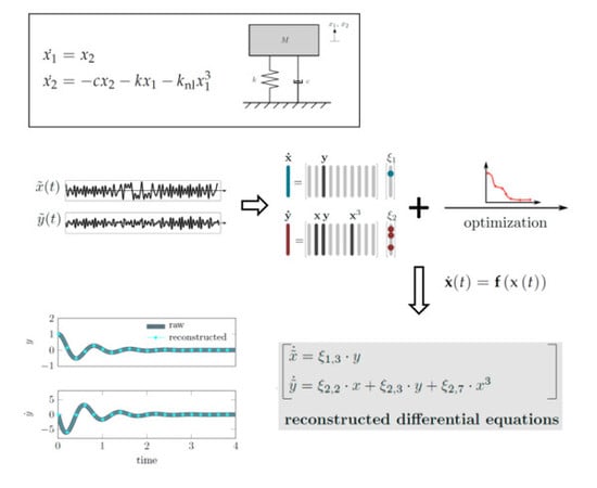
Next, the SINDy framework, as described in detail by Brunton et al. [15], is briefly introduced here, with focus on its interface to nonlinear optimization techniques. The procedure of SINDy is depicted in Figure 1. Here, only time-continuous physical flows of the type
are considered. The system states as well as their temporal derivatives are assumed to be accessible, while the underlying system is unknown. For instance, the system states can be measured during vibration experiments and their derivatives can be approximated numerically. Then, a library of nonlinear functions is compiled. The central objective of the reconstruction is to approximate from Equation (1) with as few terms as possible from the functions library, which is to find a sparse representation in the space of possible candidate functions. The state measurements and derivatives for time instances are collected in matrices and , respectively. To reconstruct the underlying system of differential equations, the over-determined system of equations
is evaluated using the function library for each system state. The central idea of SINDy is then to solve the resulting system of equations using a sparse regression approach. In contrast to classical solution schemes, such as least-squares algorithms, this procedure promotes sparsity in the coefficient matrix , which provides the best solution to the over-determined system. As a result, , which is the underlying dynamical system, is approximated by only a few functions from the library of ansatz functions. Hence, the solution to the reconstruction problem is sparse with respect to many possible candidate functions to approximate the nonlinear relation between system states and derivatives. The reconstructed set of differential equations can be read directly from the non-zero entries in the solution
where denotes the evaluation of the symbolic library of nonlinear functions and the reconstructed state. Essentially, each coefficient vector defines the linear combination of nonlinear functions for each state of the system:
Here, denotes one of the k ansatz functions, such as a quadratic polynomial , in —see also the example in Figure 1. The reconstruction result, i.e., the set of governing differential equations, is built from the sparse coefficient matrix and the library of nonlinear functions. This system of equations can then be subjected to further analysis, such as forward time integration or bifurcation analysis. In this work, we use the time integration of the reconstructed equations to compare the reconstructed dynamics to the observed dynamics , i.e., the input of SINDy, to define a measure for the reconstruction error estimate .
2.2. Time-Delay Embedding
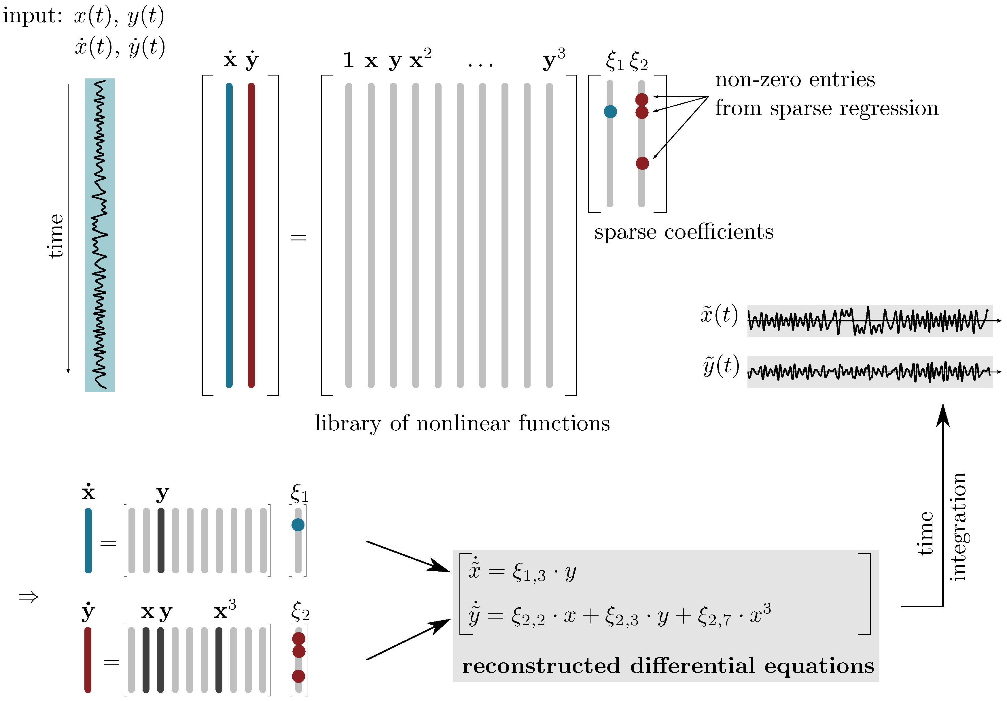
In measurements, data is limited to a finite number of signals points. Hence, only a fraction of the relevant dynamical states of a dynamical system can be measured in laboratory experiments. Time delay embedding allows for the reconstruction of the phase space of a deterministic motion that is observed in a uni-variate fashion. Takens’s theorem [18] guarantees that, for strictly deterministic processes, the trajectories in the reconstructed space have the same geometrical and dynamical properties as in the true phase space. Hence, time-delay embedding enables us to unfold the dynamics on an attractor, the invariant set, that is encoded in a single scalar time measurement. Then, the reconstructed attractor’s properties, so-called invariant measures, can be studied, which include so-called static quantities like the correlation dimension or dynamic quantities like the Lyapunov spectrum [19,20]. Time-delay embedding, given by
essentially re-arranges the scalar time series via sampling into a m-variate time series . Here, denotes the delay, which measures the distance of successive entries that are arranged to the instantaneous state vector of embedding dimension m—see Figure 2. The embedding parameters are obtained sequentially. First, the optimal delay value is derived from the temporal correlations present in the time series . The aim is to find temporally maximal de-correlated state space vectors. Hence, common approaches for deriving involve the first zero of the signal’s auto-correlation function (ACF) or the first minimum of the auto-mutual information (AMI) function which takes also nonlinear correlations into account. The embedding dimension must be chosen to be larger than twice the attractor’s dimension. For example, the motion on a limit cycle, i.e., a one-dimensional attractor, has to be embedded into two dimensions to fully unfold the attractor. While there exist multiple approaches to estimate the embedding dimension, the false nearest neighbor (FNN) algorithm is the standard tool for deriving the global dimension m [20,21,22]. The FNN algorithm iteratively increases the embedding dimension and at the same time tracks neighborhood relations in the m-dimensional phase space. False nearest neighbors are defined as states that are neighbors in dimension m but lose their neighborhood relation once the embedding dimension is increased to . The fraction of false nearest neighbors measures the overall share of those points on all state space vectors. Once the attractor is fully unfolded, states remain neighbors even if the dimension is further increased. Hence, the required embedding dimension is characterized by a low fraction of false neighbors in the m-dimensional reconstructed phase space. In this work, we employ time-delay embedding to reconstruct multivariate trajectories from uni-variate time series measurements. Additionally, the SINDy-reconstructed dynamics can be compared to measured dynamics by employing embedding parameters as error metric, cf. [23].
2.3. Uncertainty Suppressing Numerical Differentiation
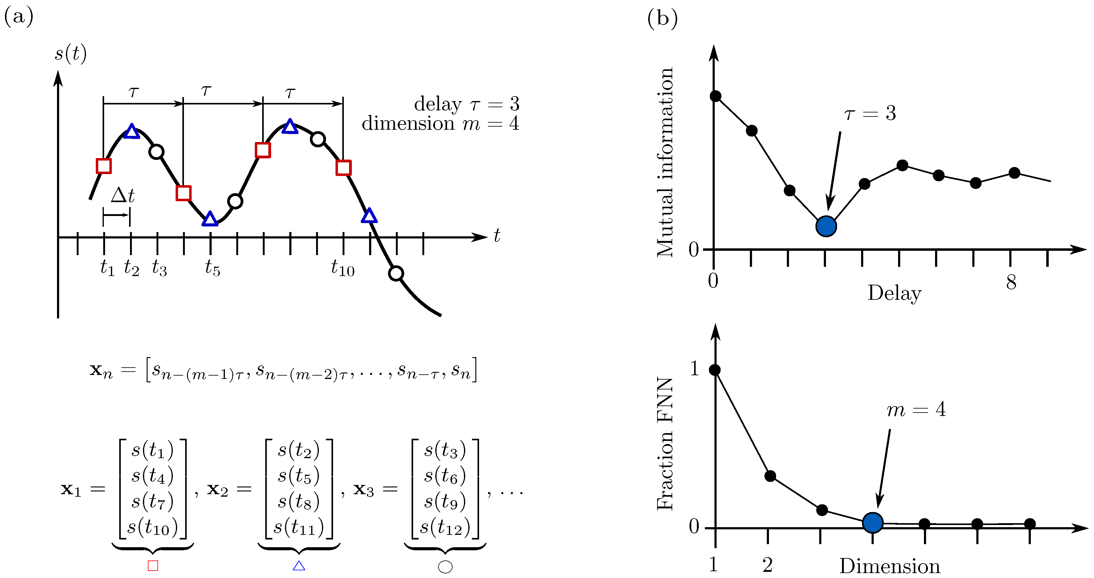
Besides all states, SINDy also requires the states’ time derivatives, either measured or generated numerically. Classical numerical differentiation schemes, such as finite differences, exhibit noise amplification—as a rule of thumb, accuracy decreases by one order of magnitude per differentiation [24]. As measurements are always contaminated with noise, a differentiation scheme is required that is particularly robust to account for this additional loss of accuracy. We employ Total Variation Regularized Numerical Differentiation, TVRegDiff, as introduced by [25] and proposed in [15], to be used within SINDy. The central idea of this differentiation scheme is to regularize the differentiation itself by balancing (a) the irregularity introduced by the derivative and (b) the error introduced by the smoothing property using a regularization parameter. Hence, this regularization parameter, denoted as , plays a crucial role. In the following, we propose an integrated and completely data-driven approach for choosing an appropriate for the specific data under study. In fact, the regularized derivative can serve as a filtering method. The regularization can then be utilized to also dampen noise in the differentiation step. The smoothed derivative is then integrated in time to yield a qualitatively enhanced (filtered) version of the input signal—see illustrative examples in Appendix A. In this work, we use TVRegDiff to compute the numerical derivatives of states with respect to time. In order to arrive at a self-consistent procedure, we substitute the original states with the time-integrated derivatives for usage in the SINDy procedure as explained before. This approach ensures that states and derivatives are matching. Here, we propose to define a time series difference measure that compares the raw input signal to the one obtained through numerical derivation and time-integration similar to Oberst et al. [17]. The search of the difference minimum will yield the optimal regularization parameter—see Figure 3. In order to reduce boundary effects at the beginning and end of each time series, the five first and last samples are discarded after differentiation.
2.4. Time Series Comparison Measures
This work extracts differential equations from time series input data. Hence, appropriate error measures have to be chosen to compare the reconstructed dynamics with the input data and thus quantify the reconstruction quality. Particularly, the set of reconstructed ODEs can be integrated in time (setting the initial value to the first input data entry) to create the reconstructed time series. Depending on the qualitative character of the time series and the specific reconstruction purpose, the reconstruction error needs to be defined. This objective represents an analogon to research fields of time series classification and time series feature engineering, where finding discriminative features forms the central methodical challenge [26,27,28]. The types of features, and thus possible candidates for definition of the reconstruction error, can be clustered as follows:
- Instance-based schemes that compare contemporaneous pairs of time series instances. In the simplest case, sequences are subtracted from each other. Modifications and advanced approaches include warping methods that add more flexibility and the ability to also take into account phase shifts.
- Higher-level features based on transforms, sampling strategies or correlation measures. Examples include statistical moments and linear transforms, such as the Fourier transform. Time series comparison is then performed based on features extracted from the transforms, such as the standard deviation or major periodicities.
- Quantifiers for qualitative behavior, mostly borrowed from nonlinear time series analysis and complexity sciences [29]. Here, the actual shape of the sequence is rather irrelevant. Instead, the qualitative nature of the dynamics encoded in the time series is of interest: dynamical invariants quantify the degree of regularity, entropy, or fractal properties of the sequence when studied in a dynamical framework, cf. [17].
Depending on the specific signal, reconstruction purpose and availability of data, any of the aforementioned features may be chosen to quantify the reconstruction error between the input and SINDy-reconstructed time series. In this work, we use the cumulative difference between reconstructed and original signal as a measure for instance-based reconstruction error due to its higher robustness, computational efficiency, and simplicity of implementation compared to e.g., recurrence plot-based measures [17].
2.5. Constrained Nonlinear Optimization
The sparse regression solution of the over-determined SINDy system of equations is not continuous in the sense of the coefficient matrix , which is a function of the sparsity parameter . This means that a fixed set of coefficients will result from a range of sparsification levels . If is increased, at some point, an additional coefficient entry will be set to zero. Until then, the coefficients remain constant. As a result, SINDy may be able to find the correct locations of non-zero coefficient entries, but not their optimal absolute value. We propose to use a nonlinear optimization scheme to fine-tune the entries in the sparse coefficient matrix found by SINDy. In this work, the Matlab routine fmincon is employed to run the optimization using the sequential quadratic programming (sqp) method. For each non-zero coefficient, we prescribe a lower and upper bound. Then, the optimizer finds the optimal set of coefficients with respect to the cost function, which measures the difference between input signal and reconstruction signal. Hence, the SINDy results represent the first approximation of the reconstruction and the nonlinear optimization fine-tunes the model for the best fit. Depending on the specific reconstruction objective, the cost function may be formulated such that it penalizes complexity and nonlinearities, promotes matching spectral properties [30], or improves other characteristics of the reconstructed model.
2.6. Models Used
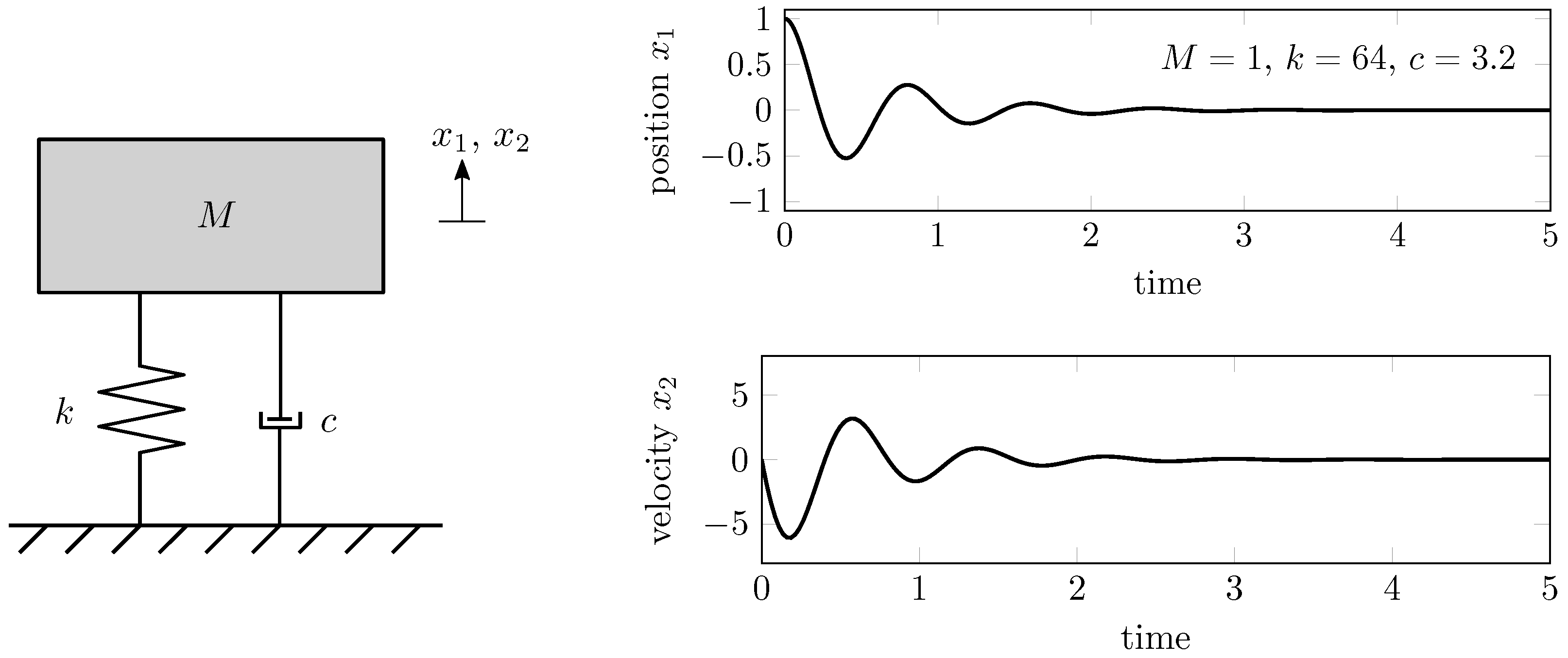
We employ a linear, 1-DOF, viscously damped mechanical oscillator to illustrate the automation and optimization extensions of SINDy. Special focus is put on the short and highly transient nature of ring-down data, i.e., impulse-response-type time series data. As a reference, the oscillator is defined as shown in Figure 4. Owing to high damping levels, there are usually only a few significant oscillations. Hence, determining classical features of ring-down data, such as the decay rate, may be challenging and prone to errors. In the following, we discuss the reconstruction in the phase space, which is represented by a first-order description of the form
This dynamical system is integrated in time for 4 s using a sampling time of s. If not denoted differently, a unit initial deflection is prescribed, i.e., . For the sake of clearer notation, we discard the physical units in the following discussions.
3. Results
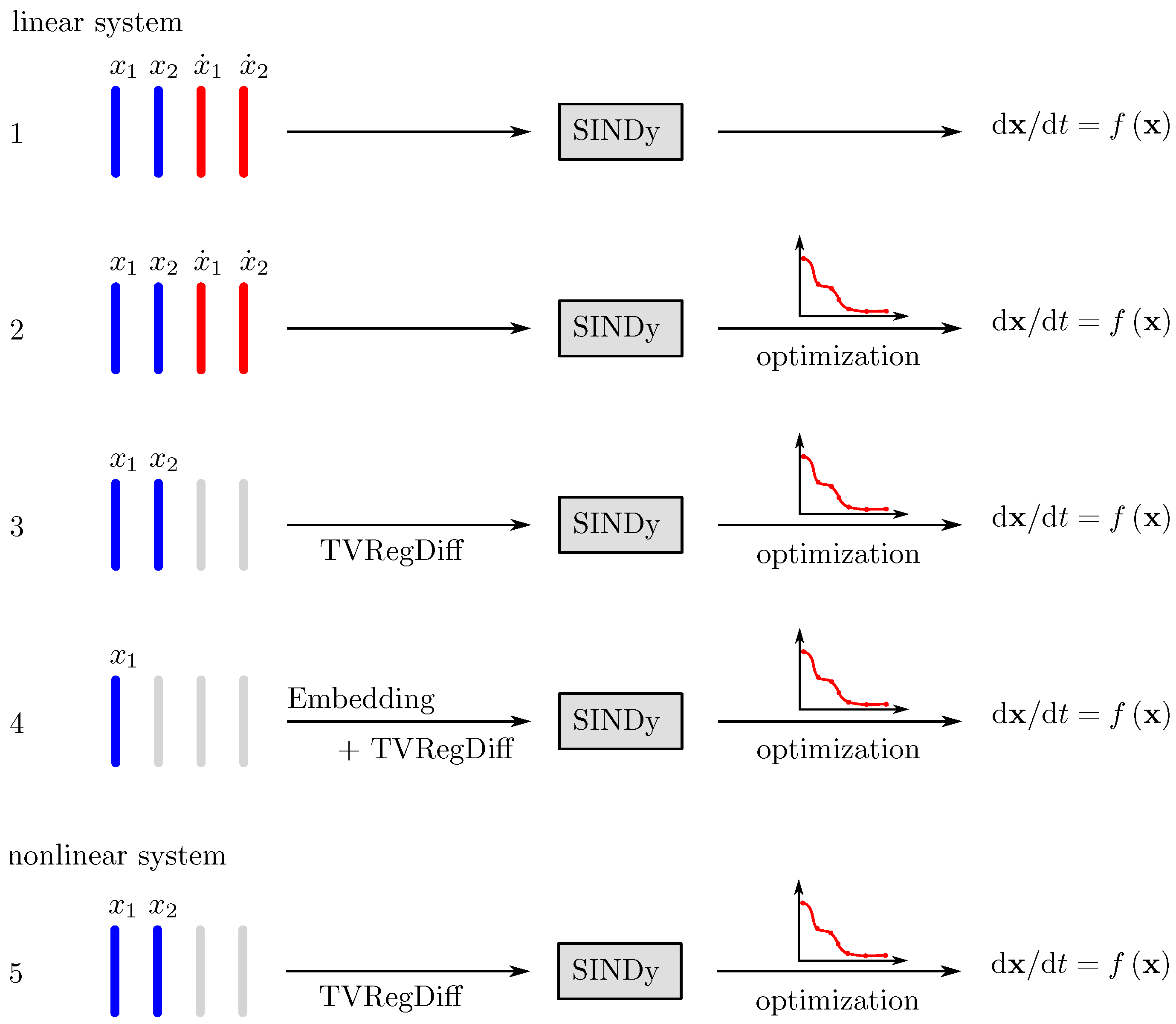
We elaborate on the proposed SINDy extensions using the example of the mechanical oscillator that oscillates freely. In the first step, the linear damped oscillator is subjected to the SINDy reconstruction for various degrees of input information level. The complexity of the reconstruction task is increased incrementally. First, the analytical derivatives are replaced by the regularized derivatives. Then, only the first state is recorded, which requires reconstructing the second state using time delay embedding. Secondly, we illustrate how the optimization procedure can improve both the reconstruction quality and the simplicity of the reconstructed models. Finally, a cubic stiffness term is introduced and identified by the proposed methods. These cascades of decreasing amounts of information available to SINDy are illustrated in Figure 5.
3.1. Instance-Based Error Measure
As the error measure, we employ the cumulative absolute Euclidean distance, given by
throughout the following discussion. For each DOF, the difference is computed between the true and reconstructed states per time step . Then, all differences are added up to form the scalar error measure . To achieve a balanced error measure, each time series of length N is normalized by the respective maximum of the true states per DOF. Hence, differences in position and velocity are weighted equally in the error measure and do not depend on the actual value range per DOF.
3.1.1. Providing Full Information: All States and Analytical Derivatives
Initially, all information is provided for SINDy: position and velocity signals as well as their derivatives are provided from the time integration of the equations of motion. As we provide a library of polynomials up to order , the exact coefficients should be found by SINDy. However, as the parameter remains the sparsification level, which has to be defined according to the length, the sampling time, the nonlinear function library and the qualitative nature of the dynamics. Following the previous illustrations, the sparsification parameter is varied in the full range between non-zero entries (NZE) of to NZE . Meanwhile, the error measure is computed from the time domain solutions of instantaneous SINDy results. Then, the optimal sparsification parameter is chosen such that it minimizes the error measure. The resulting SINDy reconstruction is integrated in time and compared to the input signal—see Figure 6. The result of SINDy matches perfectly with the analytical expression for the oscillator. Even though polynomials up to order were permitted, the optimal sparsification level yields the correct first-order differential equations and with coefficients equaling zero for all other entries, thus an NZE fraction of . As the error is close to machine precision, we do not need to further tune the non-zero coefficients, regardless of whether or not the true solution of the input signal is known.
3.1.2. Providing Less Information: All States and Numerical Derivatives
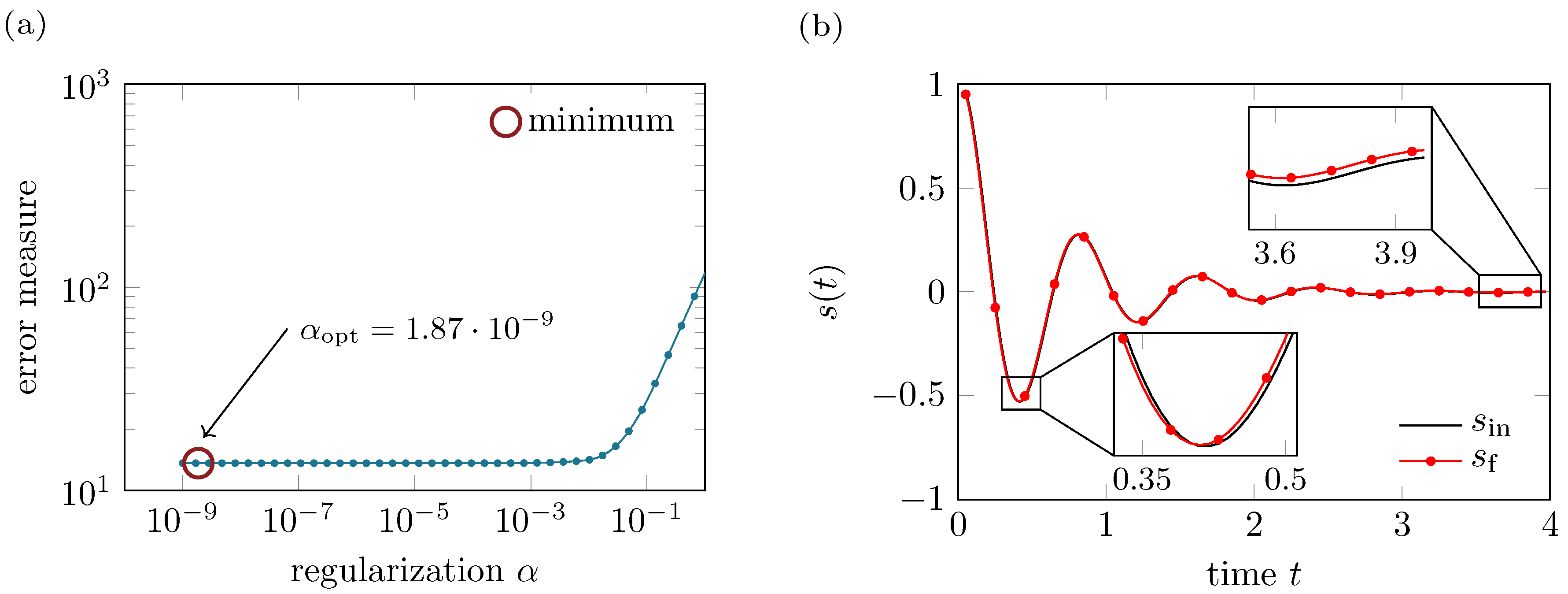
Analytical derivatives will hardly be available for an analysis as proposed here. In other words, if states and derivatives were available, there would be different solutions to find the best system of differential equations that links states with derivatives. Hence, in this scenario, we record only the states and and compute their derivatives using TVRegDiff. Therefore, the regularization parameter , has to be set prior to applying SINDy. Here, we consider noise-free signals, which makes the selection of rather straightforward. Following the description illustrated in Figure 3, we adapt the regularization such that it minimizes the difference between an input state and the state which is obtained after time integration of the numerical derivative—see Figure 7. When dealing with noise-contaminated signals, this is a semi-automated procedure that must be supervised by the user in order to make use of the filtering property of regularized derivatives, depicted in Appendix A.
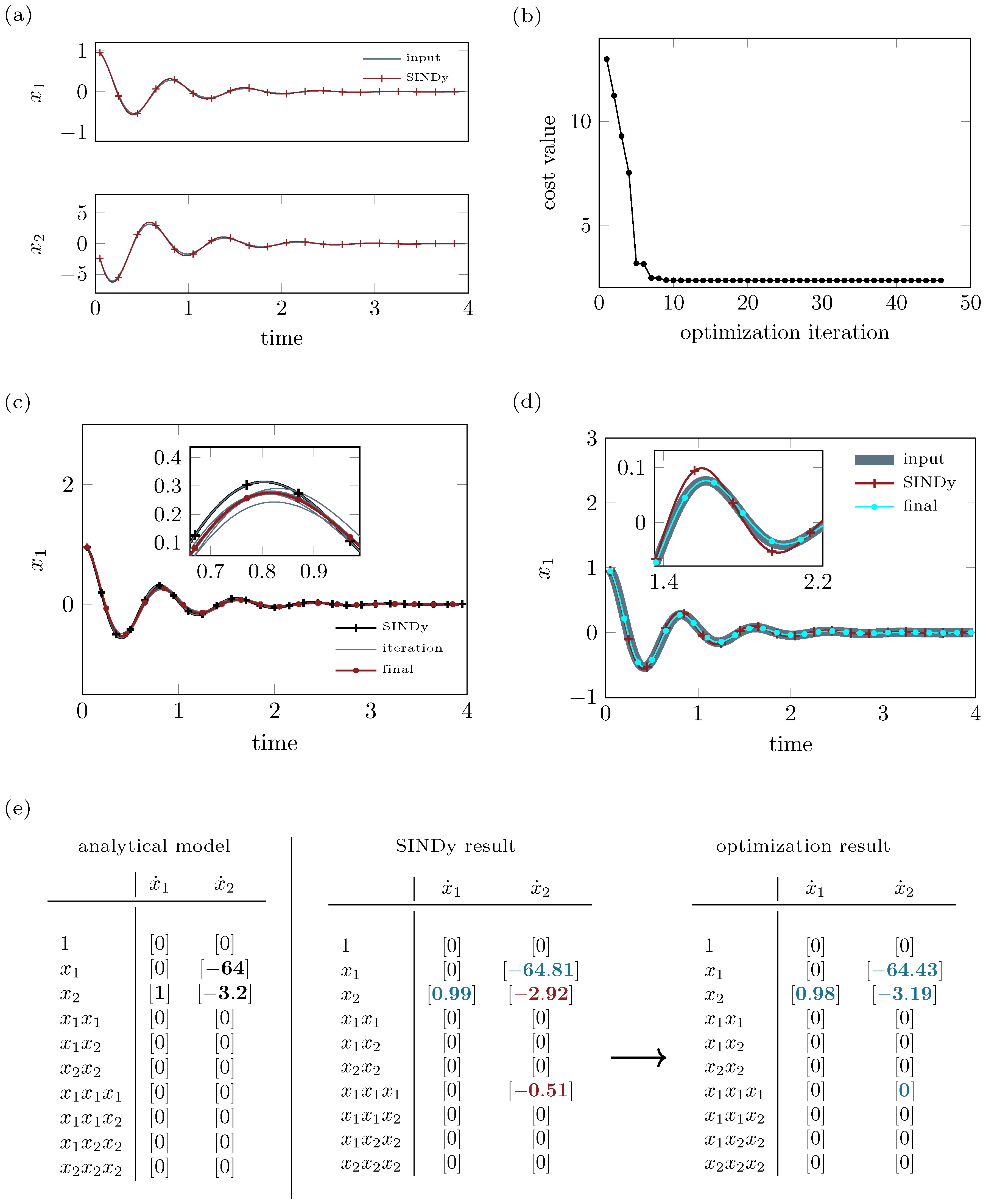
The filtered states, that is the time integrated numerical derivatives, are fed as input to the SINDy procedure along with the numerical derivatives. Using a maximal polynomial order , the sparse reconstruction is obtained following the procedure elaborated before. The best reconstruction is obtained for a sparsification parameter . The reconstructed time signals for and match well with the input signals—see Figure 8a. Out of the 20 possible coefficients, there are four non-zero entries: , . The cubic term represents an artefact that was introduced by SINDy: compared to the true system of equations, one can observe that the linear system’s eigenfrequency is slightly too large (), while the damping term is slightly smaller (), which explains the additional cubic stiffness term. This cubic term creates larger restoring forces and thus compensates for the lack of damping in the system. As the reconstruction error is rather small, and the reconstructed dynamics are sparse in the admissible nonlinear function library space, one may finish the reconstruction at this point.
However, we strive for an even smaller reconstruction error, fewer model terms and a test for nonlinearity. In particular, the latter objective may be of interest for various studies in system identification scenarios. In structural dynamics modeling, the degree of linearity is a point of crucial importance. Since linear systems obey the superposition principle, analysis of these systems can be performed with ease using a variety of established methods. Strongly nonlinear systems, on the other hand, require more complex analytical methods and can exhibit a profusion of qualitatively different dynamics that typically have not been understood as thoroughly as those of linear systems. Hence, in the current case, it might be interesting to see whether the cubic stiffness term is a decisive model parameter, or if the system can be modeled in linear fashion instead.
A central contribution of our work is the extension of the SINDy reconstruction with a nonlinear optimization procedure. The optimization problem is formulated such that the non-zero coefficients are subjected to a bounded optimization with respect to a global cost function that measures the difference of input and reconstructed time signals. The non-zero entries (NZE) in found by SINDy represent the starting point for the optimization, which is permitted to change the NZE values within prescribed boundaries and . The optimization boundaries are set in relative fashion, i.e., allowing for a certain fraction of change with respect to the initial value. However, to promote sparsification during the optimization, we set one of the boundaries to zero. This approach, which allows for further elimination of model parameters, corresponds to the dropout or pruning procedure, a well-known concept of complexity reduction in artificial neural networks [31]. Here, we allow a maximal relative change of according to
In our case, the non-zero entries in obtained by SINDy are the coefficients of in the first differential equation and those of , and in the second differential equation. Figure 8b depicts the optimization iterations of the bounded nonlinear optimization. The error measure decays quickly within the first ten iterations. Only slight adaptations are made in the following iterations before the optimization algorithm finishes at 48 iterations. When observed in the time domain, the optimization iterations are not visible in the full-scale time signal but can be identified through high magnification of the peak regions—see Figure 8c. The final minimisation result is then compared to the input signal, i.e., the reconstruction aim, and the SINDy result in Figure 8d. Through optimization, the reconstruction error has been reduced by to . While the reconstruction has been enhanced, the coefficient matrix has also become sparser thanks to this method: The auxiliary cubic stiffness term that was computed by SINDy is erased by the optimization, which makes use of the dropout option discussed before. The reconstructed set of differential equations after optimization is very similar to the analytical model which was used to create the input data—see Figure 8e.
3.1.3. Providing Less Information: State Space Reconstruction and Numerical Derivatives
In the next step, the amount of information provided by the signal input is further reduced. In real measurements, only a few measurement points are available for data acquisition. Therefore, only a fraction of the active degrees of freedom will be measured and available to the reconstruction procedure. We mimic this situation by restricting the input data to a single scalar time series, e.g., of the oscillator. The missing information about other relevant degrees of freedom in the true phase space has to be reconstructed using time delay embedding. Then, TVRegDiff allows for computing the corresponding derivatives that can be used for the SINDy reconstruction with subsequent coefficient optimization.
The embedding parameters , are found for the time series by the first zero of the auto-correlation function and by the false nearest neighbor algorithm—see Figure 9. The resulting trajectories , in the reconstructed phase space and their respective numerical derivatives are used as inputs to SINDy.
The optimized SINDy reconstruction is computed for polynomials varying from degrees to . For each configuration, the sparsity as well as the reconstruction error estimate between trajectories and their reconstruction is computed. The corresponding sets of ODEs are listed in Table 1. Generally speaking, the reconstructed ODEs will not mimic the analytical oscillator as a result of the embedding step. The reconstruction of the trajectories maps the input to another space and, therefore, the resulting states cannot be compared directly to the analytical model. In contrast, the general structure of the dynamical system as well as nonlinearity serve as viable parameters for comparison.
The previous study involving both true model states exhibits a reconstruction error of . In the current study with less information, reconstruction errors of the same order of magnitude can be observed. As the polynomial degree is increased, the reconstruction error decreases slightly before it saturates for . The coefficient matrices exhibit predominantly constant entries beginning with the simplest model, where . As a result of this trend and the low reconstruction error, one can conclude that a reconstruction using only linear combinations of the monomials and is sufficient. However, since the original analytical model in this investigation was the simple linear oscillator, the resulting linear reconstruction is not very surprising. Still, the processes of embedding and numerical differentiation could have introduced artefacts that would have increased the model complexity after reconstruction. Depending on a specific objective, one may use the linear, or also the nonlinear models that arise from this study. The latter models show a smaller reconstruction error, while the number of non-zero entries increases. This means that SINDy arrives at better reconstructions with an increasing number of terms and, as a result, greater model complexity. Thus, both the reconstruction error and the model complexity have to be balanced. For a specific application, either of those objectives may be favored.
In conclusion, SINDy is able to reconstruct dynamical models that reproduce the observed dynamics to a high degree, even if only a limited amount of input information is provided. In this case, a single state of the mechanical oscillator suffices to reconstruct a dynamical model that captures the salient feature of the dynamics and exhibits low reconstruction errors for a linear model. This result is promising for the application of the proposed methods to real experimental impulse data, which offer limited access to the states of the system and thus require embedding approaches.
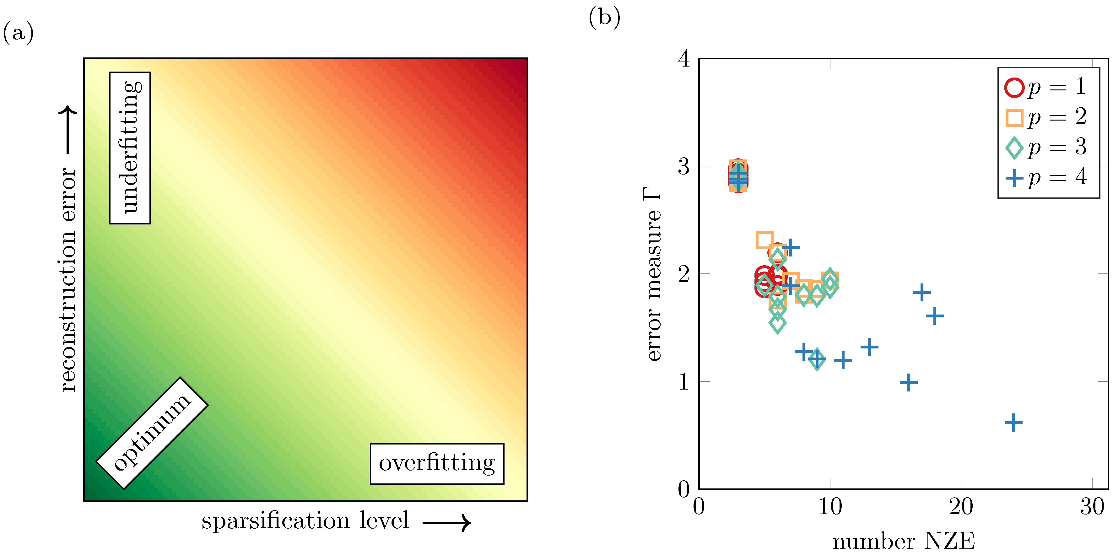
3.2. Balancing Reconstruction Error and Model Complexity
As illustrated in the previous study, reconstruction error and model complexity represent conflicting objectives when dealing with incomplete or noisy data. We classify those conflicting objectives in the framework of under- and over-fitting models, which is a classical framework in system identification and machine learning research. The number of non-zero coefficients in the reconstructed set of ODEs is a proxy for the model complexity. Hence, each SINDy model can be located in the plane spanned by model complexity and reconstruction error—see Figure 10a. Re-visiting the assumption of sparse dynamics, models of low complexity and low reconstruction error are the optimal solution to the time series based reconstruction challenge. A simple model with high reconstruction error does not capture all of the salient dynamics of the input and is thus under-fitted. On the contrary, if high complexity is required to obtain a low reconstruction error, the model may over-fit the dynamics and is unlikely to yield a generally applicable result.
To display a sample case for selecting an optimal trade-off between model complexity and reconstruction error, we revisit the reconstruction from limited input data. In the previous study, the time delay embedding was computed from the first state of the analytical oscillator. In measurements, one will most likely measure a combination of the system’s states rather than a single active degree of freedom. Thus, we study how the composition of the measured signal impacts the reconstruction error. The input to the time delay embedding is now an aggregate of both states and according to , where the scaling parameter prescribes the mixing ratio of both states. To study the effect of different input information, polynomial orders up to are studied and is varied in the range with a step size of . The resulting reconstruction results are displayed in Figure 10b. The best reconstructions, consisting of low complexity models with low error, are found for . Lower polynomial orders result in simple but imprecise reconstructions, while is prone to over-fitting, i.e., generating models of high complexity that reproduce the given data well, but generalize weakly. Depending on the specific purpose of the reconstruction, either configuration may be favorable. Still, the illustration of the resulting models in the complexity-error plane helps to find the optimal choice of parameters such as the number of candidate functions in the library .
3.3. Model Identification Studies
For illustrative purposes, we simulate three qualitatively different model identification scenarios. First, data is generated for different system configurations driven by a control parameter. This control parameter is then identified in the reconstructed models. Second, reconstruction models are built for data that stems from the same system, but for different initial conditions. This case is designed to represent multiple measurements that contain different amounts of information about a given dynamical system. Finally, data are generated for a linear and weakly nonlinear system configuration. Here, we illustrate the potential of the proposed methods to serve as a test for nonlinearity.
3.3.1. Identification of Parameter Dependencies
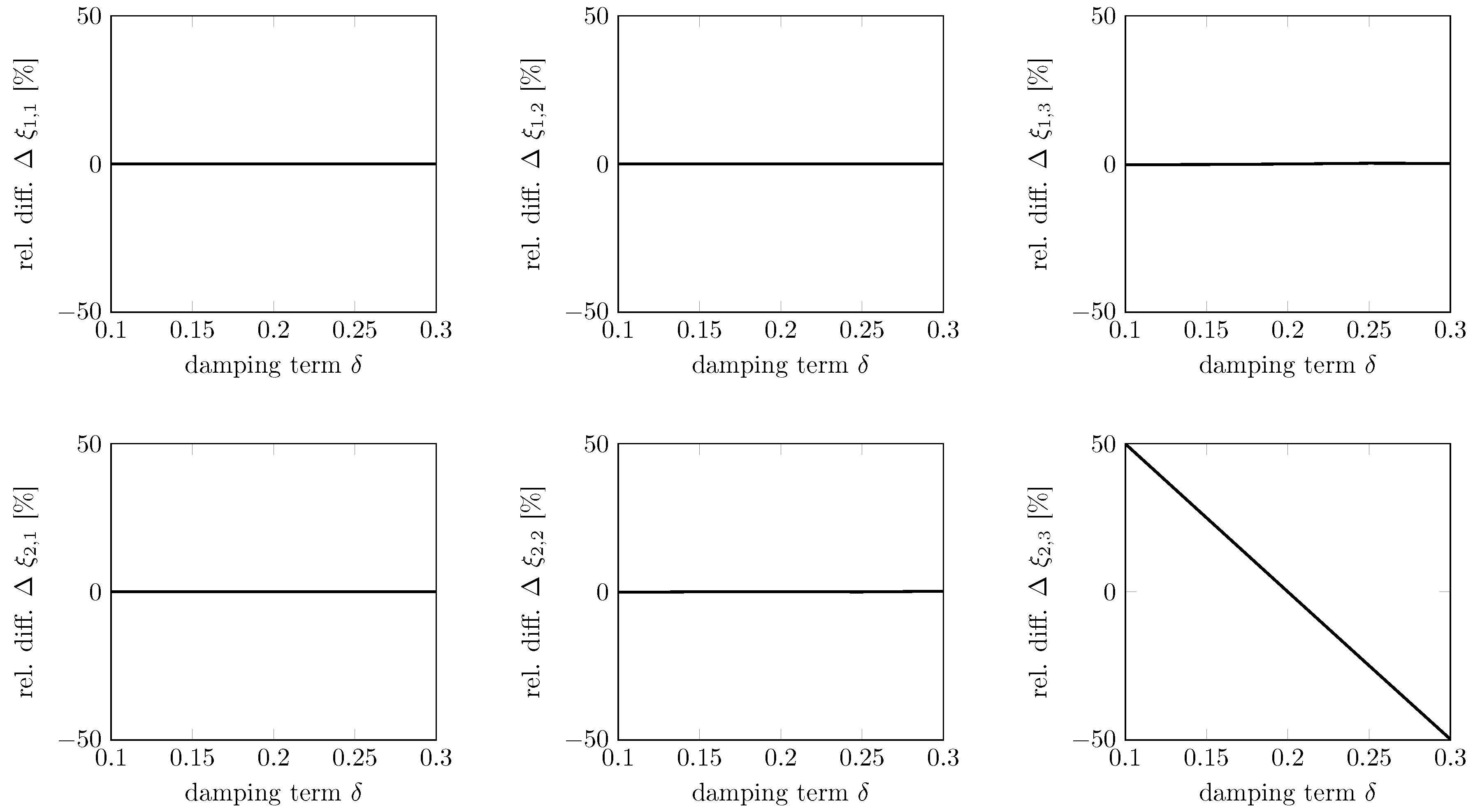
In this study, the damping term is varied as a control parameter in the range of . Optimized reconstruction models are created from each input time series and the non-zero coefficient matrix entries are recorded. As the reference system configuration, the standard value is selected. Figure 11 depicts the relative change of each coefficient relative to the reference model. The two states , are used with polynomial degree such that six ODE coefficients result. It can be observed that five out of those six coefficients remain constant throughout the control parameter variation, while only changes significantly. Hence, the control parameter variation can be traced back to a single term in the reconstructed models. Consequently, this model parameter has to be studied in order to investigate control parameter changes in simulations. Of course, this scenario is well-constructed to illustrate a simple parameter dependency. However, the concept of tracking model parameters along with control parameters can be transferred directly to more complicated and more realistic parameter identification challenges. Moreover, this procedure can be used in an inverse sense to identify the model parameters that are invariant under parameter changes.
3.3.2. Robust Model Parameter Identification
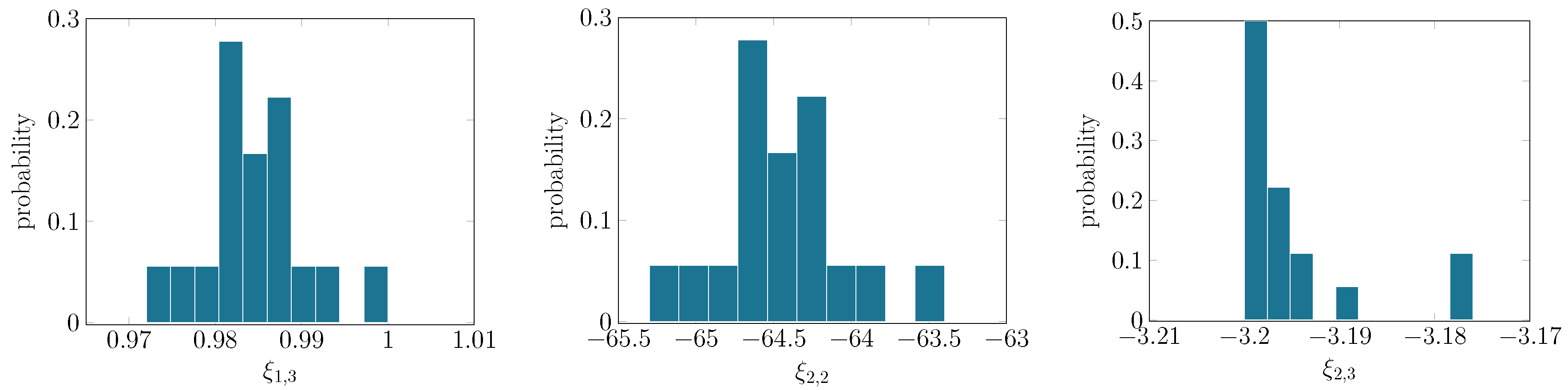
Imagine testing a dynamical system using hammer impacts. Naturally, each excitation is different, but the dynamical system remains the same. We try to simulate this situation by varying the initial conditions for creating various input time series of the oscillator. Each realization stems from the same dynamical system, and thus we look for one model reconstructed from all data. For each piece of input data, an optimized SINDy model is computed and coefficient values are recorded. Figure 12 depicts histograms of the relevant, i.e., non-zero, coefficient matrix entries. In order to define the optimal model, one would select representative coefficient values, such as the most frequent or median values, from these histograms and form the final coefficient matrix. Here, the final model with , and would result from the most frequent coefficient values, which is a good approximation of the true analytical model used to generate the data (, , ). This procedure is different from the one proposed by Brunton et al. [15], where all data are stacked into a large data matrix and subjected to a single SINDy reconstruction. Due to the highly transient nature and resulting spectra of amplitudes of the data recorded in this work, we suggest deriving multiple models instead.
3.3.3. Test for Nonlinearity
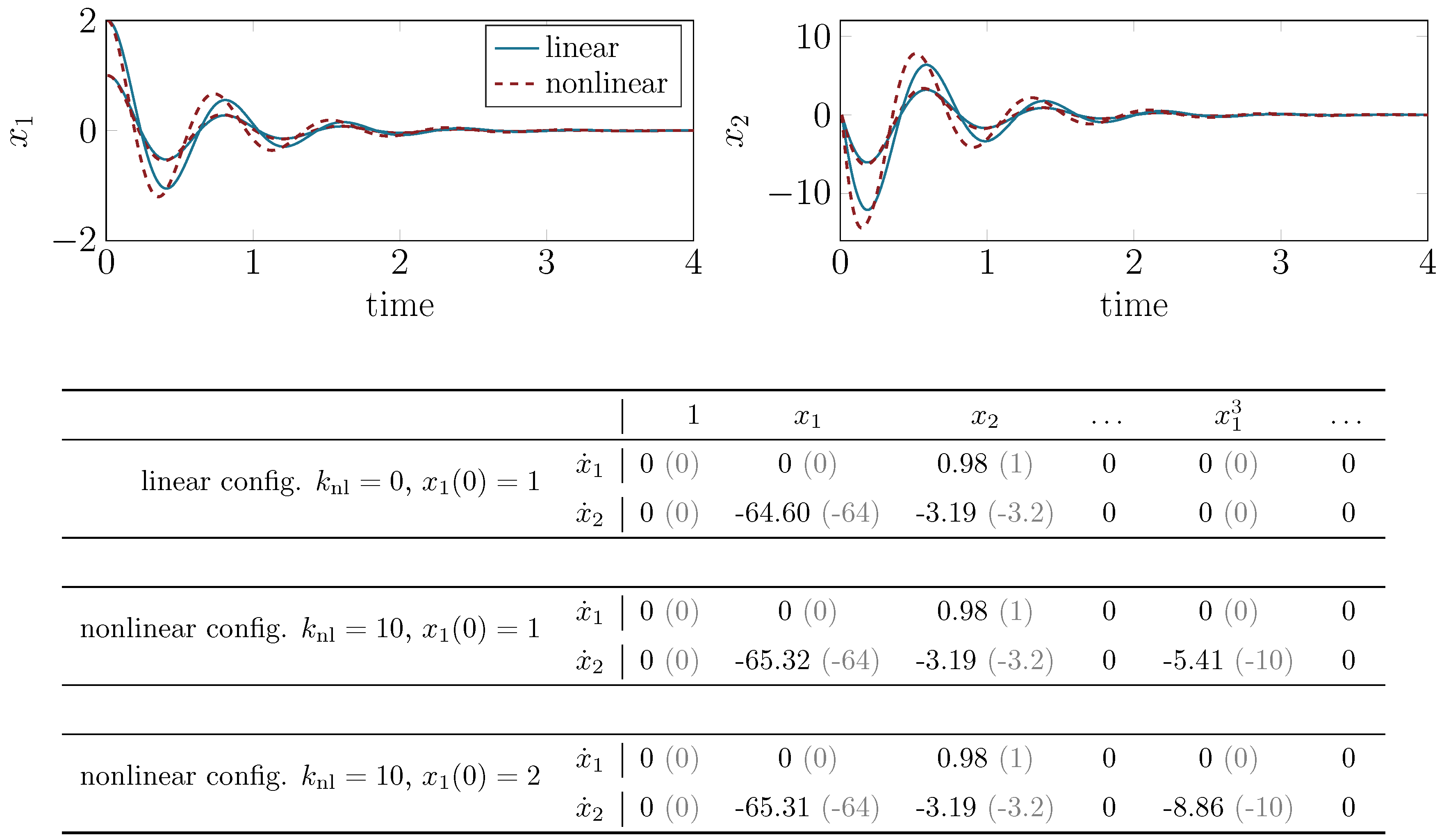
In order to extend the findings from the given mechanical oscillator to nonlinear dynamics, we introduce an additional cubic stiffness term such that the governing equations read
The reference configuration is given by , and, in the nonlinear configuration, , if not denoted differently. Figure 13 displays the analytical states , for both the linear as well as nonlinear configuration of the 1-DOF oscillator. For small initial values, the nonlinearity is practically inactive and only minimal differences to the linear configuration can be observed in the time domain. However, the SINDy reconstruction clearly identifies a non-zero entry for the ansatz polynomial and thus allows for testing for nonlinearity, even if the time traces are barely distinguishable in the time domain. However, while the cubic stiffness parameter is underestimated, the linear stiffness is overestimated. This result matches well with the understanding of linearization of the cubic stiffness for small displacement values. As the initial displacement is increased, the nonlinearity becomes active and visible in time domain and the SINDy model exhibits a cubic stiffness term that is closer to that of the analytical model.
3.4. Feature Generation for Unsupervised Time Series Classification Tasks
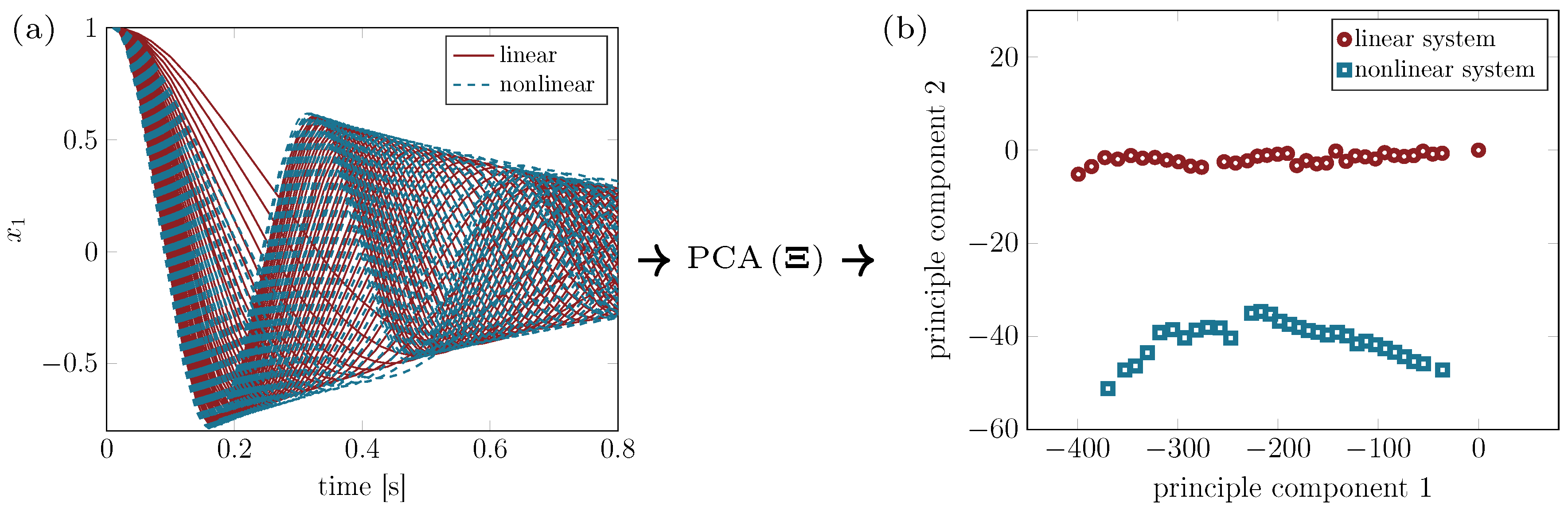
Finally, we illustrate a sample case for using the SINDy reconstruction as a feature generator. In various fields of research, the discrimination of time series data forms the central challenge for both supervised as well as unsupervised classification tasks. To mimic the situation of an unsupervised classification task, we compute various ring-down time series data from varying model configurations. We then compute the reconstruction and employ the resulting ODE coefficients as features for describing the input data. These features are then used to solve the classification task in this setting. Particularly, the linear stiffness is varied over a wide range of values , while the nonlinear stiffness is kept constant for two different scenarios. First, the oscillator is considered in the linear configuration, i.e., . Then, a constant cubic stiffness of is considered. For each of those configurations, 40 time-series realizations ( s) with varying linear stiffness terms are created. Then, optimized SINDy reconstruction models are computed for each input. The highest polynomial order is set to and both states , from the analytical model are used as input to the reconstruction. The first epochs of all the 80 input time series of state are depicted in Figure 14. While it may seem easy to distinguish some of the linear system responses from the nonlinear responses, most of the time traces overlap. Due to rather small amplitudes and strong damping, classical methods for describing and discriminating those dynamics may fail to cluster the data into two distinct groups representing the linear and nonlinear configurations of the underlying model, as shown in the previous discussion. In particular, the nonlinearity may be negligible for higher linear stiffness terms, which makes it nearly impossible to distinguish the system response from the raw time series data stemming from a purely linear system. We employ the proposed methods to derive optimized SINDy reconstructions and then collect the resulting ODE coefficients into a matrix. In five cases, the SINDy ODE reconstruction was unstable, and was hence discarded. The resulting matrix has 75 rows, each corresponding to one reconstruction, and 20 columns, each of which result from the coefficients for the library of polynomials up to the third order for two states. For each observation, we treat the coefficients as discriminative features for describing the input time series data. The 20-dimensional feature space is reduced to two dimensions by principle component analysis (PCA). Hence, for each observation, two generalized features are given by the projection of the features onto the first and second principle components ()—see Figure 14. In this feature space, two distinct clusters form, which, since we know the label for each observation, can be traced back to the underlying dynamical systems. The features created by our methods exhibit variance in mainly one direction for the linear oscillator, which corresponds to the variation of the linear stiffness term. On the contrary, the features derived for the signals stemming from the nonlinear systems show additional variance in the second principle component, which makes them distinguishable from the linear system features. We note that the linear stiffness has been varied over one order of magnitude for both cases in order to complicate the classification task. Still, our results illustrate that the unsupervised time series classification task can be solved using the SINDy reconstruction models as feature generator in a highly automated fashion. The gaps in both clusters at stem from the five invalid SINDy reconstructions. Naturally, this approach can be employed equally for supervised classification tasks, by assigning a label to an unknown input according to a-priori knowledge that was gathered from labeled training data.
4. Conclusions
In this work, we propose several extensions to the SINDy method, which allows for reconstructing differential equations from time series input data. The reconstruction is sparse in the space of possible candidate functions and thus represents a minimal model for the observed dynamics. The main contribution of this work comprises of a highly automated parameter selection approach and of a sophisticated optimization procedure to fine-tune reconstructed models. Special focus is put on short and highly transient time series data as commonly obtained from impulse response and ring-down vibration measurements. Employing a 1-DOF oscillator, we illustrate the proposed extensions as well as common use-cases and challenges that may also arise and be observed in real-life laboratory data. These situations include limited data availability, noise contamination, and uncertain parameters of the dynamical system under study. The main findings and features of the proposed framework are summarized as follows:
- Reconstruction of dynamic minimal models: The sparse regression reconstructs systems of differential equations from time series data. Hence, these equations can be studied and analyzed by classical methods and provide detailed insight into the governing dynamics underlying an observation.
- Model reconstruction for limited input data: The proposed framework automates and optimizes the model reconstruction procedure while being suited well for accommodating limited data quality resulting from the amount of information, noise contamination, and unknown model dimensions.
- Test for nonlinearity: The qualitative character of the underlying dynamical system can be estimated in terms of linearity and type and degree of nonlinearity by inspecting the set of reconstructed differential equations.
- Model identification and model updating methods: The optimized reconstruction allows for identification of terms that depend explicitly on parameters that are prescribed or measured during experimentation. After identifying those terms in the reconstructed ODEs, uncertainty and bifurcation studies can be used in predictive modeling approaches to design safe and efficient structures without extensive testing.
- Time series feature generation for classification and regression tasks: The reconstructed models represent features that are discriminative and possibly superior to classical time series features for uni-variate, short and highly transient input data.
Future research will use the proposed framework of methods to identify dynamic minimal models and change the system underlying these minimal models taking real-life vibration measurements, such as hammer-impact testing during modal analysis of mechanical structures.
Author Contributions
Conceptualization, M.S., S.O. and N.H.; Software and Investigation, M.S.; Writing—Original Draft Preparation, M.S.; Writing—Review and Editing, S.O. and N.H.; Supervision and Project Administration, S.O. and N.H.
Funding
This research was funded by Deutsche Forschungsgemeinschaft (DFG) within the priority program ’calm, smooth, smart’ under grant HO 3852/21-1. M.S. acknowledges the financial support S.O. over the UTS Centre for Audio, Acoustics and Vibration (CAAV) international visitor funds.
Acknowledgments
The Matlab code provided by Steven Brunton was used to generate the SINDy reconstruction. The authors would like to thank Edgar Hoover for his assistance in improving the clarity of the manuscript.
Conflicts of Interest
The authors declare no conflict of interest. The funders had no role in the design of the study; in the collection, analyses, or interpretation of data; in the writing of the manuscript, or in the decision to publish the results.
Abbreviations
The following abbreviations are used in this manuscript:
| DOF | Degree Of Freedom |
| NZE | Non-Zero Entries |
| ODE | Ordinary Differential Equation |
| SINDy | Sparse Identification of Nonlinear Dynamics |
| TVRegDiff | Total Variation Regularized Numerical Differentiation |
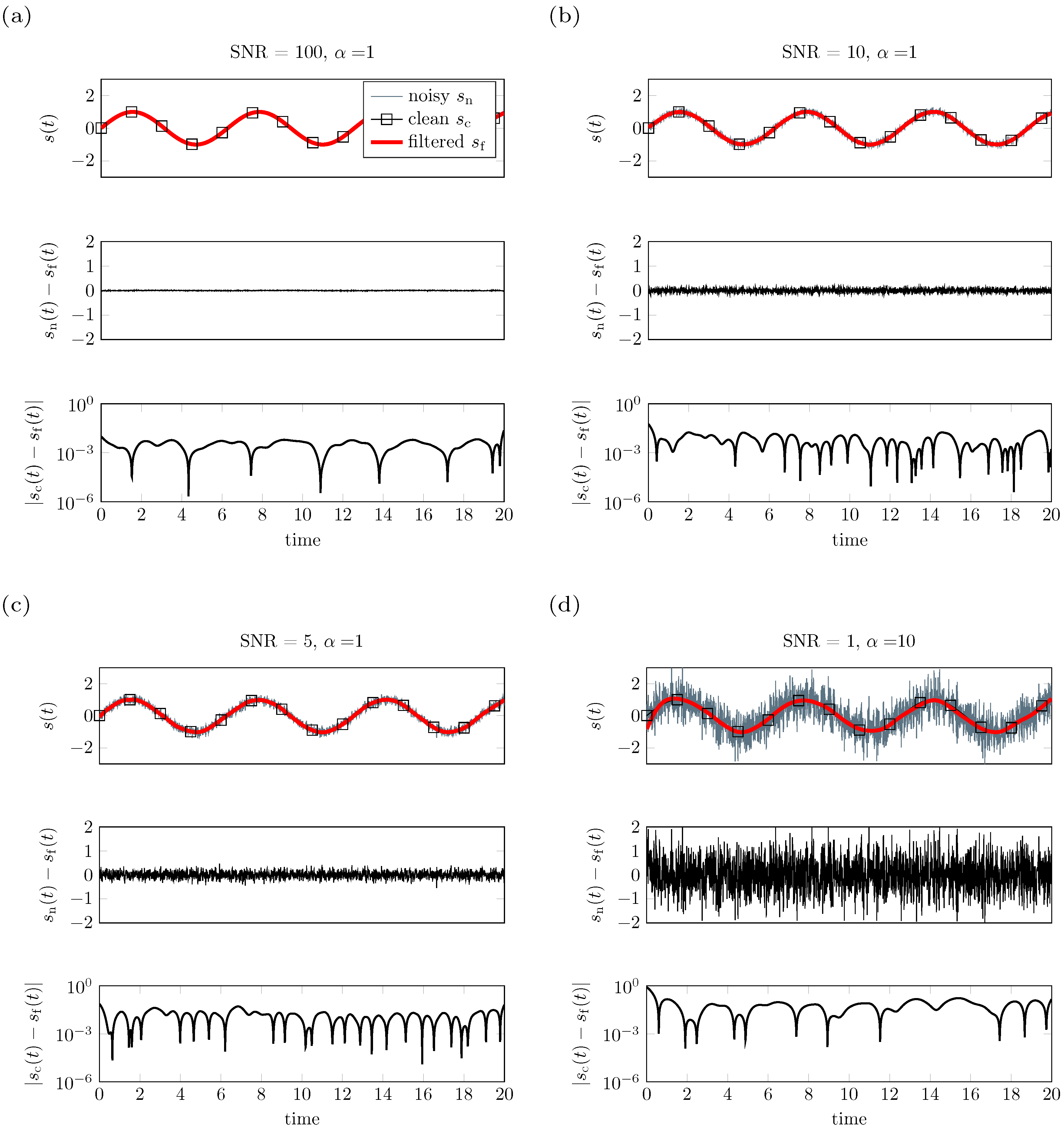
Appendix A. The Filtering Property of TVRegDiff Numerical Derivation Schemes
Figure A1 illustrates the filtering property of the TVRegDiff scheme with appropriate choice of the regularization parameter for different signal-to-noise ratios.
Figure A1.
Filtering by integration of regularized derivatives: different noise levels applied to sinusoidal oscillation . Clean signal is indicated by , noisy (signal-to-noise ratio SNR) signal by and filtered signal, which is obtained from time integration of the numerical derivative, . Regularization parameters were employed for computing derivatives using TVRegDiff, and SNR values decrease from (a) to (d)

References
- Ondra, V.; Sever, I.A.; Schwingshackl, C.W. A method for non-parameteric identification of nonlinear vibration systems with asymmetric restoring forces from a resonant decay response. Mechan. Syst. Signal Process. 2019, 114, 239–258. [Google Scholar] [CrossRef]
- Ondra, V.; Sever, I.A.; Schwingshackl, C.W. A method for detection and characterisation of structural nonlinearities using the Hilbert transform. Mechan. Syst. Signal Process. 2017, 83, 210–227. [Google Scholar] [CrossRef]
- Pesaresi, L.; Stender, M.; Ruffini, V.; Schwingshackl, C.W. DIC Measurement of the Kinematics of a Friction Damper for Turbine Applications. In Dynamics of Coupled Structures, Volume 4, Conference Proceedings of the Society for Experimental Mechanics Series; Springer: Cham, Switzerland, 2017; pp. 93–101. [Google Scholar]
- Kurt, M.; Chen, H.; Lee, Y.; McFarland, M.; Bergman, L.; Vakakis, A. Nonlinear system identification of the dynamics of a vibro-impact beam: Numerical results. Arch. Appl. Mech. 2012, 82, 1461–1479. [Google Scholar] [CrossRef]
- Farrar, C.R.; Worden, K. An introduction to structural health monitoring. Philos. Trans. R. Soc. A 2007, 365, 303–315. [Google Scholar] [CrossRef] [PubMed] [Green Version]
- Nuawi, M.Z.; Bahari, A.R.; Abdullah, S.; Ariffin, A.K.; Nopiah, Z.M. Time Domain Analysis Method of the Impulse Vibro-acoustic Signal for Fatigue Strength Characterisation of Metallic Material. Procedia Eng. 2013, 66, 539–548. [Google Scholar] [CrossRef]
- Crutchfield, J.P.; McNamara, B.S. Equations of motion from a data series. Complex Syst. 1987, 1, 121. [Google Scholar]
- Kurt, M.; Eriten, M.; McFarland, M.; Bergman, L.; Vakakis, A. Methodology for model updating of mechanical components with local nonlinearities. J. Sound Vib. 2015, 357, 331–348. [Google Scholar] [CrossRef]
- Moore, K.; Kurt, M.; Eriten, M.; McFarland, M.; Bergman, L.; Vakakis, A. Direct detection of nonlinear modal interactions from time series measurements. Mechan. Syst. Signal Process. 2018. [Google Scholar] [CrossRef]
- González-García, R.; Rico-Martínez, R.; Kevrekidis, I.G. Identification of distributed parameter systems: A neural net based approach. Comput. Chem. Eng. 1998, 22, S965–S968. [Google Scholar] [CrossRef]
- Raissi, M.; Karniadakis, G.E. Hidden physics models: Machine learning of nonlinear partial differential equations. J. Comput. Phys. 2018, 357, 125–141. [Google Scholar] [CrossRef] [Green Version]
- Gouesbet, G.; Letellier, C. Global vector-field reconstruction by using a multivariate polynomial L2 approximation on nets. Phys. Rev. E 1994, 49, 4955–4972. [Google Scholar] [CrossRef]
- Liu, W.-D.; Ren, K.F.; Meunier-Guttin-Cluzel, S.; Gouesbet, G. Global vector-field reconstruction of nonlinear dynamical systems from a time series with SVD method and validation with Lyapunov exponents. Chin. Phys. 2003, 12, 1366. [Google Scholar]
- Wang, W.X.; Yang, R.; Lai, Y.C.; Kovanis, V.; Grebogi, C. Predicting catastrophes in nonlinear dynamical systems by compressive sensing. Phys. Rev. Lett. 2011, 106, 154101. [Google Scholar] [CrossRef] [PubMed]
- Brunton, S.L.; Proctor, J.L.; Kutz, J.N. Discovering governing equations from data by sparse identification of nonlinear dynamical systems. Proc. Natl. Acad. Sci. USA 2016, 113, 3932–3937. [Google Scholar] [CrossRef] [PubMed]
- Rudy, S.H.; Brunton, S.L.; Proctor, J.L.; Kutz, J.N. Data-driven discovery of partial differential equations. Sci. Adv. 2017, 3, e1602614. [Google Scholar] [CrossRef]
- Oberst, S.; Stender, M.; Baetz, J.; Campbell, G.; Lampe, F.; Morlock, M.; Lai, J.C.; Hoffmann, N. Extracting differential equations from measured vibro-acoustic impulse responses in cavity preparation of total hip arthroplasty. In Proceedings of the 15th Experimental Chaos and Complexity Conference, Madrid, Spain, 4–7 June 2018. [Google Scholar]
- Takens, F. Detecting strange attractors in turbulence. In Dynamical Systems and Turbulence; Springer: Berlin/Heidelberg, Germany, 1981; pp. 366–381. [Google Scholar]
- Kantz, H.; Schreiber, T. Nonlinear Time Series Analysis; Cambridge University Press: Cambridge, UK, 2003. [Google Scholar]
- Oberst, S.; Lai, J.C. A statistical approach to estimate the Lyapunov spectrum in disc brake squeal. J. Sound Vib. 2015, 334, 120–135. [Google Scholar] [CrossRef]
- Abarbanel, H.D.I.; Brown, R.; Sidorowich, J.J.; Tsimring, L.S. The analysis of observed chaotic data in physical systems. Rev. Mod. Phys. 1993, 65, 1331–1392. [Google Scholar] [CrossRef]
- Kennel, M.B.; Brown, R.; Abarbanel, H.D.I. Determining embedding dimension for phase-space reconstruction using a geometrical construction. Phys. Rev. A 1992, 45, 3403–3411. [Google Scholar] [CrossRef]
- Oberst, S.; Baetz, J.; Campbell, G.; Lampe, F.; Lai, J.C.; Hoffmann, N.; Morlock, M. Vibro-acoustic and nonlinear analysis of cadavric femoral bone impaction in cavity preparations. Int. J. Mech. Sci. 2018, 144, 739–745. [Google Scholar] [CrossRef]
- Gilmore, R.; Lefranc, M.; Tufillaro, N.B. The Topology of Chaos. Am. J. Phys. 2003, 71, 508–510. [Google Scholar] [CrossRef]
- Chartrand, R. Numerical Differentiation of Noisy, Nonsmooth Data. ISRN Appl. Math. 2011, 2011, 1–11. [Google Scholar] [CrossRef] [Green Version]
- Fulcher, B.D.; Jones, N.S. Highly Comparative Feature-Based Time-Series Classification. IEEE Trans. Knowl. Data Eng. 2014, 26, 3026–3037. [Google Scholar] [CrossRef] [Green Version]
- Bagnall, A.; Lines, J.; Hills, J.; Bostrom, A. Time-Series Classification with COTE: The Collective of Transformation-Based Ensembles. IEEE Trans. Knowl. Data Eng. 2015, 27, 2522–2535. [Google Scholar] [CrossRef]
- Fulcher, B.D.; Jones, N.S. hctsa: A Computational Framework for Automated Time-Series Phenotyping Using Massive Feature Extraction. Cell Syst. 2017, 5, 527–531.e3. [Google Scholar] [CrossRef] [PubMed]
- Marwan, N.; Romano, M.C.; Thiel, M.; Kurths, J. Recurrence plots for the analysis of complex systems. Phys. Rep. 2007, 438, 237–329. [Google Scholar] [CrossRef]
- Stender, M.; Papangelo, A.; Allen, M.; Brake, M.; Schwingshackl, C.; Tiedemann, M. Structural Design with Joints for Maximum Dissipation. In Shock & Vibration, Aircraft/Aerospace, Energy Harvesting, Acoustics & Optics; Springer: Cham, Switzerland, 2016; Volume 9, pp. 179–187. [Google Scholar]
- Srivastava, N.; Hinto, G.; Krizhevsky, A.; Sutskever, I.; Salakhutdinov, R. Dropout: A simple way to prevent neural networks from overfitting. J. Mach. Learn. Res. 2014, 15, 1929–1958. [Google Scholar]
Figure 1.
Schematic illustration of the SINDy procedure, closely related to the illustration given in [15]. System states and their derivatives are required as time series input. Then, a library of nonlinear candidate functions is compiled. The resulting over-determined system of equations is solved by sparsity-promoting regression techniques to yield a sparse reconstruction of the underlying dynamical system in terms of ordinary differential equations.

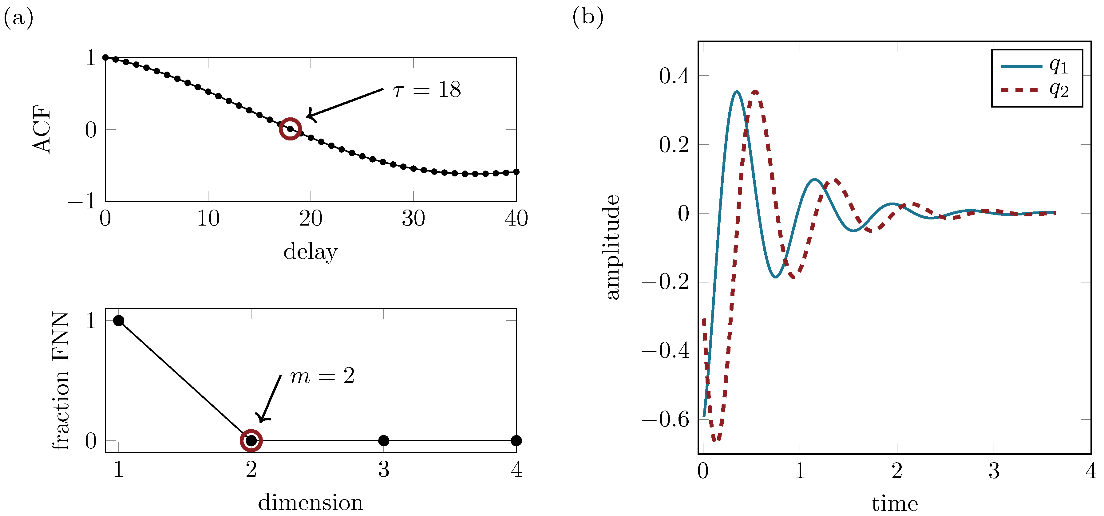
Figure 2.
(a) schematic illustration of the time delay embedding procedure using the embedding parameters and m that were obtained from (b), the first minimum of the auto-mutual information function and the dimension with vanishing fraction of false nearest neighbors, respectively.
Figure 2.
(a) schematic illustration of the time delay embedding procedure using the embedding parameters and m that were obtained from (b), the first minimum of the auto-mutual information function and the dimension with vanishing fraction of false nearest neighbors, respectively.

Figure 3.
Integrated approach for finding the optimal regularization parameter for the numerical differentiation using TVRegDiff: the time integration of the numerical derivative allows for deriving an error measure that can be used to adapt the regularization parameter for noise contaminated input time series.

Figure 4.
Linear 1-DOF viscously damped oscillator and time traces of position and velocity for an initial deflection of .
Figure 4.
Linear 1-DOF viscously damped oscillator and time traces of position and velocity for an initial deflection of .

Figure 5.
Overview of the studies performed using the 1-DOF oscillator. The reconstruction task becomes increasingly challenging due to decreasing amounts of information available and added nonlinearity.
Figure 5.
Overview of the studies performed using the 1-DOF oscillator. The reconstruction task becomes increasingly challenging due to decreasing amounts of information available and added nonlinearity.

Figure 6.
(a) Finding the optimal sparsification level as minimum of the error measure; (b) comparison of input signal to SINDy reconstruction with maximal polynomial order .
Figure 6.
(a) Finding the optimal sparsification level as minimum of the error measure; (b) comparison of input signal to SINDy reconstruction with maximal polynomial order .

Figure 7.
Comparison of the input time signal and the filtered one obtained through time integration of the regularized numerical derivative. (a) Error measure as a function of the regularization parameter and (b) the resulting signal for an optimal regularization .
Figure 7.
Comparison of the input time signal and the filtered one obtained through time integration of the regularized numerical derivative. (a) Error measure as a function of the regularization parameter and (b) the resulting signal for an optimal regularization .

Figure 8.
Two-step reconstruction procedure: (a) comparison of input data and SINDy reconstruction that used regularized numerical derivatives; (b,c) iterations of the bounded optimizer on the non-zero coefficients to reduce the difference between input and reconstruction signal; (d) result of the two-step reconstruction and (e) evolution of the coefficient matrices obtained from SINDy and the optimization procedure in comparison to the analytical oscillator model that generated the initial input signals.

Figure 9.
(a) Determining the embedding parameters as a first zero of the ACF and vanishing fraction of the FNN algorithm for ; (b) resulting trajectories and in the reconstructed phase space.
Figure 9.
(a) Determining the embedding parameters as a first zero of the ACF and vanishing fraction of the FNN algorithm for ; (b) resulting trajectories and in the reconstructed phase space.

Figure 10.
(a) Balancing model complexity and reconstruction error: depending on a specific parameter selection, the reconstructed equations may represent under-, well-, and over-fitting models, as depicted in this schematic representation; (b) depicts the resulting model characteristics for various input configurations and varying polynomial orders of the nonlinear functions library. In this case, most of the configurations result in very complex, i.e., unsatisfactory, reconstructions.

Figure 11.
Relative deviation of the reconstructed ODE coefficients from the reference configuration as function of the control parameter . As a reference, is chosen to identify those terms that are invariant under the parameter change.
Figure 11.
Relative deviation of the reconstructed ODE coefficients from the reference configuration as function of the control parameter . As a reference, is chosen to identify those terms that are invariant under the parameter change.

Figure 12.
Model identification from various measurements: Histograms of the non-zero coefficient matrix entries resulting from 36 realizations of the same linear oscillator for all possible combinations of the initial conditions with highest polynomial order . For model coefficient identification, the most frequent or median coefficient value may be selected from the histograms. The underlying analytical model is given by , , .

Figure 13.
Comparison of linear and nonlinear 1-DOF oscillators in time domain (top) and in terms of the optimized SINDy reconstruction models (bottom). The analytical model parameters are indicated by the coefficient values given in brackets in the table. Only non-vanishing terms are displayed here for a maximal polynomial order of .

Figure 14.
(a) 40 time series realizations for various linear stiffness terms for the linear () and the nonlinear configuration (). The resulting SINDy coefficient entries are used as descriptive features for classification of the input data; (b) using the principle component analysis, the feature space is reduced to two dimensions to find two clusters that can be traced back to the character of the underlying dynamical model that generated the input data.


Table 1.
Coefficient matrices for optimized SINDy reconstruction for maximal polynomial degrees p and resulting reconstruction error . The states and were taken from the time delay embedded signal and used as input signals—see Figure 9. Terms that are not displayed became zero in this analysis. The reconstruction for failed with an error of and 13 NZE after optimization.
| 1 | Other Terms | |||||||
|---|---|---|---|---|---|---|---|---|
| , | 0 | −0.74 | −5.84 | - | - | - | - | |
| −0.008 | 10.60 | −2.45 | - | - | - | - | ||
| , | 0 | −0.75 | −5.82 | −0.06 | - | - | - | |
| −0.007 | 10.62 | −2.45 | 0 | - | - | - | ||
| , | 0 | −0.81 | −5.84 | −0.13 | 0.51 | 0.16 | - | |
| 0 | 10.60 | −2.39 | 0 | 0 | 0 | - | ||
| , | 0 | −0.85 | −5.86 | 0 | 0.7080 | 0 | −0.96 −1.44 | |
| 0 | 10.54 | −2.36 | 0 | 0 | 0 | 0 |
© 2019 by the authors. Licensee MDPI, Basel, Switzerland. This article is an open access article distributed under the terms and conditions of the Creative Commons Attribution (CC BY) license (http://creativecommons.org/licenses/by/4.0/).
Share and Cite
MDPI and ACS Style
Stender, M.; Oberst, S.; Hoffmann, N. Recovery of Differential Equations from Impulse Response Time Series Data for Model Identification and Feature Extraction. Vibration 2019, 2, 25-46. https://doi.org/10.3390/vibration2010002
AMA Style
Stender M, Oberst S, Hoffmann N. Recovery of Differential Equations from Impulse Response Time Series Data for Model Identification and Feature Extraction. Vibration. 2019; 2(1):25-46. https://doi.org/10.3390/vibration2010002
Chicago/Turabian StyleStender, Merten, Sebastian Oberst, and Norbert Hoffmann. 2019. "Recovery of Differential Equations from Impulse Response Time Series Data for Model Identification and Feature Extraction" Vibration 2, no. 1: 25-46. https://doi.org/10.3390/vibration2010002