Electromagnetic Vacuum Densities Induced by a Cosmic String

Abstract

We investigate the influence of a generalized cosmic string in $(D+1)$-dimensional spacetime on the local characteristics of the electromagnetic vacuum. Two special cases are considered with flat and locally de Sitter background geometries. The topological contributions in the vacuum expectation values (VEVs) of the squared electric and magnetic fields are explicitly separated. Depending on the number of spatial dimensions and on the planar angle deficit induced by the cosmic string, these contributions can be either negative or positive. In the case of the flat bulk, the VEV of the energy–momentum tensor is evaluated as well. For the locally de Sitter bulk, the influence of the background gravitational field essentially changes the behavior of the vacuum densities at distances from the string larger than the curvature radius of the spacetime.

1. Introduction

The formation of topological defects is one of the interesting consequences of symmetry breaking phase transitions in the early Universe. Depending on the topology of the vacuum manifold, these are domain walls, strings, monopoles and textures. Among them, cosmic strings have been of increasing interest due to the importance that they may have in cosmology [1]. This class of defects are sources of a number of interesting astrophysical effects such as the generation of gravitational waves, high-energy cosmic rays, and gamma ray bursts. Another interesting effect is the influence of cosmic strings on the temperature anisotropies of the cosmic microwave background radiation. More recently, a mechanism for the generation of the cosmic string type objects is proposed within the framework of brane inflation [2,3].

Depending on the underlying microscopic model, the cosmic strings can be either nontrivial field configurations or more fundamental objects in superstring theories. In the simplest theoretical model describing straight cosmic strings, the influence of the latter on the surrounding geometry at large distances from the core is reduced to the generation of a planar angle deficit. In quantum field theory, among the most interesting effects of the corresponding nontrivial spatial topology is the vacuum polarization. This effects have been discussed for scalar, fermion and vector fields (see, for instance, references cited in [4,5]).

In the present paper, we present the results of the investigations for the influence of a cosmic string on the vacuum electromagnetic fluctuations. The vacuum expectation value (VEV) of the energy–momentum tensor for the electromagnetic field around a cosmic string in $D=3$ spatial dimensions has been obtained in [6,7] based on the Green function. For superconducting cosmic strings, assuming that the string is surrounded by a superconducting cylindrical surface, in [8] the electromagnetic energy produced in the lowest mode is evaluated. The VEVs of the squared electric and magnetic fields, and of the energy–momentum tensor for the electromagnetic field inside and outside of a conducting cylindrical shell in the cosmic string spacetime have been investigated in [9]. The corresponding VEVs, the Casimir–Polder and the Casimir forces in the geometry of two parallel conducting plates on the background of cosmic string spacetime were discussed in [10,11]. The repulsive Casimir–Polder forces acting on a polarizable microparticle in the geometry of a straight cosmic string are investigated in [12,13]. The Casimir–Polder interaction between an atom and a metallic cylindrical shell in cosmic string spacetime has been studied in [14] (see also [15]). The electromagnetic field correlators and the VEVs of the squared electric and magnetic fields around a cosmic string in background of $(D+1)$-dimensional locally de Sitter (dS) spacetime are evaluated in [16] (for quantum vacuum effects in the geometry of two straight parallel cosmic strings, see [17] and references therein).

The organization of the paper is as follows. In the next section, we present the complete set of the electromagnetic field mode functions on the bulk of a $(D+1)$-dimensional generalized cosmic string geometry. In Section 3, by using these mode functions, the VEVs of the squared electric and magnetic fields are investigated. The VEV of the energy–momentum tensor is studied in Section 4. In Section 5, we consider the VEVs of the squared electric and magnetic fields, and of the vacuum energy density for a cosmic string in locally dS spacetime. The main results are summarized in Section 6.

2. Electromagnetic Field Modes Around a Cosmic String in Flat Spacetime

In the first part of the paper, we consider a quantum electromagnetic field with the vector potential $A_{\mu }\left(x\right)$ in the background of a $(D+1)$-dimensional flat spacetime, in the presence of an infinitely long straight cosmic string with the line element

$$d{s}^2=d{t}^2-d{r}^2-r^{2}d{\varphi }^2-{\left(d\mathbf{z}\right)}^2,$$

(1)

where $\mathbf{z}=\left(z^3,...,z^D\right),$$0\le \varphi \le {\varphi }_0$ and the points $(r,\varphi ,\mathbf{z})$ and $(r,\varphi +{\varphi }_0,\mathbf{z})$ are to be identified. The geometry described by Equation (1) is flat everywhere except the points on the axis $r=0$ where one has a delta-type singularity. Though the local characteristics of the cosmic string spacetime in the region $r>0$ are the same as those in flat spacetime, for ${\varphi }_0\ne 2\pi$ these manifolds differ globally. We are interested in the influence of nontrivial topology induced by a planar angle deficit on local characteristics of the electromagnetic vacuum. In the canonical quantization procedure, we need to know a complete orthonormal set $\{A_{\left(\beta \right)\mu },A_{\left(\beta \right)\mu }^{*}\}$ of solutions to the classical field equations ${\partial }_{\nu }\left(\sqrt{\left|g\right|}{F}^{\mu \nu }\right)=0$, where $F_{\mu \nu }$ is the electromagnetic field tensor, $F_{\mu \nu }={\partial }_{\mu }{A}_{\nu }-{\partial }_{\nu }{A}_{\mu }$, and g is the determinant of the metric tensor. Here and below, the set $\left(\beta \right)$ of quantum numbers specifies the mode functions. In the Coulomb gauge one has $A_{\left(\beta \right)0}=0$, ${\partial }_l(\sqrt{\left|g\right|}{A}_{\left(\beta \right)}^l)=0$, $l=1,...,D$.

In the problem at hand, the set of quantum numbers is specified as $\left(\beta \right)=(\gamma ,m,\mathbf{k},\sigma )$. Here, $0⩽\gamma <\infty$ is the radial quantum number, $m=0,\pm 1,\pm 2,\dots$ is the azimuthal quantum number, $\mathbf{k}=(k_3,\dots ,k_D)$ is the momentum in the subspace $\left(z^3,...,z^D\right)$, and $\sigma =1,\dots ,D-1$ enumerates the polarization states. The cylindrical modes for the electromagnetic field are given by

$$\begin{array}{ccc}\hfill A_{\left(\beta \right)\mu }& =& C_{\left(\beta \right)}\left(0,\frac{iqm}{r},-r{\partial }_r,0,\dots ,0\right)J_{q\left|m\right|}\left(\gamma r\right)e^{i(qm\varphi +\mathbf{k}·\mathbf{z}-\omega t)},\sigma =1,\hfill \\ \hfill A_{\left(\beta \right)\mu }& =& C_{\left(\beta \right)}\omega \left(0,{ϵ}_{\sigma l}+i\frac{\mathbf{k}·{ϵ}_{\sigma }}{{\omega }^2}{\partial }_l\right)J_{q\left|m\right|}\left(\gamma r\right)e^{i(qm\varphi +\mathbf{k}·\mathbf{z}-\omega t)},\sigma =2,\dots ,D-1,\hfill \end{array}$$

(2)

where $l=1,\dots ,D$, $q=2\pi /{\varphi }_0$, $\omega =\sqrt{{\gamma }^2+k^2}$, $k^2={\sum }_{l=3}^D{k}_l^2$, and $J_{\nu }\left(x\right)$ is the Bessel function of the first kind. The scalar products are given as $\mathbf{k}·\mathbf{z}={\sum }_{l=3}^D{k}_l{z}^l$ and $\mathbf{k}·{\mathit{ϵ}}_{\sigma }={\sum }_{l=3}^D{k}_l{ϵ}_{\sigma l}$. For the polarization vector ${\mathit{ϵ}}_{\sigma }$, one has ${ϵ}_{\sigma 1}={ϵ}_{\sigma 2}=0$, $\sigma =2,\dots ,D-1$, and the relations

$$\begin{array}{ccc}\hfill \sum _{l,n=3}^D\left({\omega }^2{\delta }_{nl}-k_l{k}_n\right){ϵ}_{\sigma l}{ϵ}_{{\sigma }^{\prime }n}& =& {\gamma }^2{\delta }_{\sigma {\sigma }^{\prime }},\hfill \\ \hfill {\omega }^2\sum _{\sigma =2}^{D-1}{ϵ}_{\sigma n}{ϵ}_{\sigma l}-k_n{k}_l& =& {\gamma }^2{\delta }_{nl},l,n=3,...,D.\hfill \end{array}$$

(3)

The polarization state $\sigma =1$ is the mode of TE type and $\sigma =2,\dots ,D-1$ correspond to $D-2$ modes of the TM type.

The coefficients $C_{\left(\beta \right)}$ are determined by the normalization condition for vector fields. For a general background with the metric tensor $g_{ik}$ this condition is written as

$$\int d^{D}x\sqrt{\left|g\right|}{g}^{00}[A_{\left({\beta }^{\prime }\right)\nu }^{*}\left(x\right){\nabla }_0{A}_{\left(\beta \right)}^{\nu }\left(x\right)-\left({\nabla }_0{A}_{\left({\beta }^{\prime }\right)\nu }^{*}\left(x\right)\right)A_{\left(\beta \right)}^{\nu }\left(x\right)]=4i\pi {\delta }_{\beta {\beta }^{\prime }},$$

(4)

where ${\nabla }_{\mu }$ stands for the covariant derivative and ${\delta }_{\beta {\beta }^{\prime }}$ is understood as the Kronecker symbol for discrete components of the collective index $\beta$ and the Dirac delta function for the continuous ones. In the problem under consideration, by using the standard integral for the product of Bessel functions, one finds

$$|C_{\left(\beta \right)}{|}^2=\frac{q}{{\left(2\pi \right)}^{D-2}\gamma \omega },$$

(5)

for all the polarizations $\sigma =1,\dots ,D-1$.

With a given set of mode functions (Equation (2)), the VEV of any physical quantity $F\{A_{\mu }\left(x\right),A_{\nu }\left(x\right)\}$ bilinear in the field is evaluated by making use of the mode-sum formula

$$\langle 0|F\{A_{\mu }\left(x\right),A_{\nu }\left(x\right)\}|0\rangle =\sum _{\beta }F\{A_{\left(\beta \right)\mu }\left(x\right),A_{\left(\beta \right)\nu }^{*}\left(x\right)\},$$

(6)

where $|0\rangle$ stands for the vacuum state and

$$\sum _{\beta }=\sum _{\sigma =1}^{D-1}\sum _{m=-\infty }^{\infty }\int d\mathbf{k}{\int }_0^{\infty }d\gamma .$$

(7)

The expression in the right-hand side of Equation (6) is divergent and requires a regularization with the subsequent renormalization. The regularization can be done by introducing a cutoff function or by the point splitting. A very convenient tool for studying one-loop divergences is the heat kernel expansion (for a general introduction with applications to conical spaces, see [18,19]). The heat kernels of Laplacians for higher spin fields and the related asymptotic expansions on manifolds with conical singularities were studied in [20]. In the following, we use an approach based on the cutoff function. Compared with the point splitting, it essentially simplifies the calculations of the topological contributions in the VEVs of local observables.

3. VEVs of the Squared Electric and Magnetic Fields

First, we consider the VEV of the squared electric field. This VEV is obtained by making use of the mode-sum formula

$$\langle 0|E^2|0\rangle \equiv \langle E^2\rangle =-g^{00}{g}^{il}\sum _{\beta }{\partial }_0{A}_{\left(\beta \right)i}\left(x\right){\partial }_0{A}_{\left(\beta \right)l}^{*}\left(x\right).$$

(8)

Note that the VEV of the electric field squared determines the Casimir–Polder potential between the cosmic string and a polarizable particle with a frequency-independent polarizability. We will regularize the VEV by introducing the cutoff function $e^{-b{\omega }^2}$ with $b>0$ (about using this kind of cutoff function in the evaluation of the Casimir energy see, for example, [21]). Substituting the mode functions and using (3), the regularized VEV is presented in the form

$$\begin{array}{ccc}\hfill {\langle E^2\rangle }_{\mathrm{reg}}& =& \frac{4{\left(4\pi \right)}^{1-D/2}q}{\mathrm{\Gamma }(D/2-1)}\underset{m=0}{\overset{\infty }{{\sum }^{\prime }}}{\int }_0^{\infty }dk{k}^{D-3}{\int }_0^{\infty }d\gamma \frac{\gamma }{\omega }{e}^{-b{\omega }^2}\hfill \\ & & \times \left\{\left({\gamma }^2+2k^2\right)G_{qm}\left(\gamma r\right)+\left[(D-2){\gamma }^2+(D-3)k^2\right]J_{qm}^2\left(\gamma r\right)\right\},\hfill \end{array}$$

(9)

where the prime on the summation sign means that the term $m=0$ should be taken with the coefficient 1/2 and the function

$$G_{\nu }\left(x\right)={J_{\nu }^{\prime }}^2\left(x\right)+\frac{{\nu }^2}{x^2}{J}_{\nu }^2\left(x\right)$$

(10)

is introduced.

For the further transformation of the right-hand side in Equation (9), we use the integral representation

$$\frac{1}{\omega }=\frac{2}{\sqrt{\pi }}{\int }_0^{\infty }dy{e}^{-({\gamma }^2+k^2)y^2}.$$

(11)

After the evaluation of the k-integrals, one gets

$$\begin{array}{ccc}\hfill {\langle E^2\rangle }_{\mathrm{reg}}& =& \frac{2^{4-D}q}{{\pi }^{(D-1)/2}}\underset{m=0}{\overset{\infty }{{\sum }^{\prime }}}{\int }_0^{\infty }\frac{dy}{w^{D/2}}{\int }_0^{\infty }d\gamma \gamma \left[\left(D-2-w{\partial }_w\right)G_{qm}\left(\gamma r\right)\right.\hfill \\ & & \left.+\left(D-2\right)\left(\frac{D-3}{2}-w{\partial }_w\right)J_{qm}^2\left(\gamma r\right)\right]e^{-w{\gamma }^2},\hfill \end{array}$$

(12)

where $w=b+y^2$. Next, we use the integral [22]

$${\int }_0^{\infty }d\gamma \gamma e^{-w{\gamma }^2}{J}_{qm}\left(\gamma r\right)J_{qm}\left(\gamma r^{\prime }\right)=\frac{1}{2w}exp\left(-\frac{r^2+{r^{\prime }}^2}{4w}\right)I_{qm}\left(\frac{r{r}^{\prime }}{2w}\right),$$

(13)

with $r^{\prime }=r$ and with $I_{\nu }\left(x\right)$ being the modified Bessel function. The remaining integral over $\gamma$ is written as

$${\int }_0^{\infty }d\gamma \gamma e^{-w{\gamma }^2}{G}_{qm}\left(\gamma r\right)=\underset{r^{\prime }\to r}{lim}\left({\partial }_r{\partial }_{r^{\prime }}+\frac{q^2{m}^2}{r{r}^{\prime }}\right){\int }_0^{\infty }d\gamma \frac{e^{-w{\gamma }^2}}{\gamma }{J}_{qm}\left(\gamma r\right)J_{qm}\left(\gamma r^{\prime }\right).$$

(14)

By taking into account that $e^{-w{\gamma }^2}={\gamma }^2{\int }_w^{\infty }dt{e}^{-t{\gamma }^2}$ and using Equation (13), one finds

$${\int }_0^{\infty }d\gamma \frac{e^{-w{\gamma }^2}}{\gamma }{J}_{qm}\left(\gamma r\right)J_{qm}\left(\gamma r^{\prime }\right)=\frac{1}{2}{\int }_0^{1/\left(4w\right)}\frac{dx}{x}{e}^{-(r^2+{r^{\prime }}^2)x}{I}_{qm}\left(2r{r}^{\prime }x\right).$$

(15)

Substituting this into Equation (14), we obtain

$${\int }_0^{\infty }d\gamma \gamma e^{-w{\gamma }^2}{G}_{qm}\left(\gamma r\right)=\frac{u}{r^2}\left({\partial }_u+1\right)e^{-u}{I}_{qm}\left(u\right),$$

(16)

with the notation $u=r^2/\left(2w\right)$.

By taking into account Equations (13) and (16) and passing in Equation (12) from the integration over y to the integration over u, one finds

$$\begin{array}{ccc}\hfill {\langle E^2\rangle }_{\mathrm{reg}}& =& \frac{4q}{{\left(2\pi \right)}^{(D-1)/2}{r}^{D+1}}{\int }_0^{r^2/\left(2b\right)}du\frac{u^{(D-1)/2}}{\sqrt{1-2bu/r^2}}\left[\left(D-2+{\partial }_{u}u\right)\left({\partial }_u+1\right)\right.\hfill \\ & & \left.+\left(D-2\right)\left(\frac{D-3}{2}+{\partial }_{u}u\right)\right]e^{-u}\underset{m=0}{\overset{\infty }{{\sum }^{\prime }}}{I}_{qm}\left(u\right).\hfill \end{array}$$

(17)

For the further transformation, we use the formula [10,23]

$$\underset{m=0}{\overset{\infty }{{\sum }^{\prime }}}{I}_{qm}\left(u\right)=\frac{1}{q}\underset{l=0}{\overset{[q/2]}{{\sum }^{\prime }}}{e}^{ucos(2l\pi /q)}-\frac{1}{2\pi }{\int }_0^{\infty }dy\frac{sin\left(q\pi \right)e^{-ucoshy}}{cosh\left(qy\right)-cos\left(q\pi \right)},$$

(18)

where $[q/2]$ stands for the integer part of $q/2$ and the prime on the summation sign means that the terms $l=0$ and $l=q/2$ (for even values of q) should be taken with additional coefficient 1/2. In the case $q=1$ the $l=0$ term remains only. From here, it follows that the contribution of the term $l=0$ in the VEV (Equation (17)) corresponds to the VEV in flat spacetime in the absence of cosmic string. We denote the corresponding regularized VEV by ${\langle E^2\rangle }_{\mathrm{reg}}^{\left(0\right)}$. The latter is obtained from Equation (17) taking the $l=0$ term in Equation (18) instead of the series over m:

$${\langle E^2\rangle }_{\mathrm{reg}}^{\left(0\right)}=\frac{\left(D-1\right)\mathrm{\Gamma }((D+1)/2)}{2^{D-1}{\pi }^{D/2-1}\mathrm{\Gamma }(D/2)b^{(D+1)/2}}.$$

(19)

The remaining part in Equation (17) is the contribution induced by the cosmic string (topological part). This part is finite in the limit $b\to 0$ and the cutoff can be removed. We denote the topological part in the VEV of the squared electric field as ${\langle E^2\rangle }_{\mathrm{t}}$:

$${\langle E^2\rangle }_{\mathrm{t}}=\underset{b\to 0}{lim}\left[{\langle E^2\rangle }_{\mathrm{reg}}-{\langle E^2\rangle }_{\mathrm{reg}}^{\left(0\right)}\right].$$

(20)

Substituting Equation (18) into Equation (17), separating the $l=0$ term and taking the limit $b\to 0$, after the evaluation of the u-integral, for the topological contribution, we find the following result

$${\langle E^2\rangle }_{\mathrm{t}}=-\frac{\mathrm{\Gamma }(\left(D+1\right)/2)}{{\left(4\pi \right)}^{(D-1)/2}{r}^{D+1}}\left[\left(D-1\right)c_{D+1}+2\left(D-3\right)c_{D-1}\right],$$

(21)

with the notation

$$c_n\left(q\right)=\underset{l=1}{\overset{[q/2]}{{\sum }^{\prime }}}\frac{1}{{sin}^n(\pi l/q)}-\frac{q}{\pi }sin\left(q\pi \right){\int }_0^{\infty }dy\frac{{cosh}^{-n}y}{cosh\left(2qy\right)-cos\left(q\pi \right)},$$

(22)

where the prime means that for even values of q the term $l=[q/2]$ should be taken with coefficient 1/2. Note that the functions (Equation (22)) also appear in the coefficients of the heat kernel expansion in the background of cosmic string spacetime (see [24,25]).

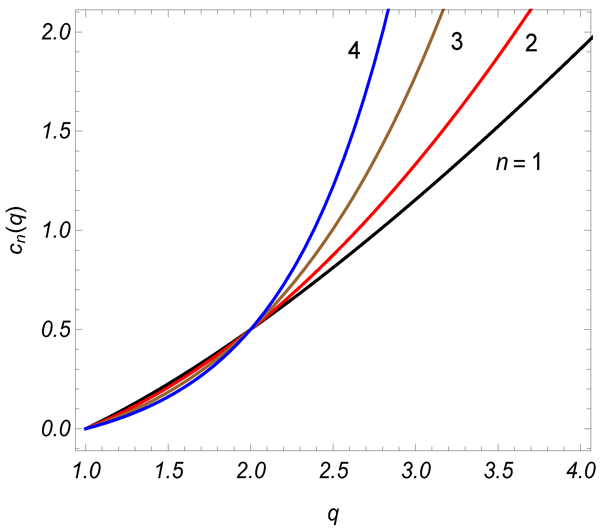
In Figure 1, we have plotted the functions $c_n\left(q\right)$ for different values of n. These functions are monotonically increasing positive functions of $q>1$. For them, one has $c_n\left(2\right)=1/2$ and $c_n\left(q\right)>c_{n+1}\left(q\right)$ for $1<q<2$. In the region $q>2$ we have $c_n\left(q\right)<c_{n+1}\left(q\right)$.

From Equation (21), we conclude that the topological part in the VEV of the squared electric field is negative for $D⩾3$ and for $q=2$ one gets

$${\langle E^2\rangle }_{\mathrm{t}}=-\frac{\mathrm{\Gamma }(\left(D+1\right)/2)}{2{\left(4\pi \right)}^{(D-1)/2}{r}^{D+1}}\left(3D-7\right),q=2.$$

(23)

For even values of n, the function $c_n\left(q\right)$ can be further simplified by using the recurrence scheme described in [26]. In particular, one has $c_2\left(q\right)=(q^2-1)/6$ and

$$\begin{array}{ccc}\hfill c_4\left(q\right)& =& \frac{q^2-1}{90}\left(q^2+11\right),\hfill \\ \hfill c_6\left(q\right)& =& \frac{q^2-1}{1890}(2q^4+23q^2+191).\hfill \end{array}$$

(24)

By using these results, one gets [9]

$${\langle E^2\rangle }_{\mathrm{t}}=-\frac{q^2-1}{180\pi r^4}\left(q^2+11\right),$$

(25)

for $D=3$ and

$${\langle E^2\rangle }_{\mathrm{t}}=-\frac{q^2-1}{1890{\pi }^2{r}^6}\left(q^4+22q^2+211\right),$$

(26)

for $D=5$. The topological part induced by the string is negative for $q>1$.

Now, we consider the VEV of the squared magnetic field, given by

$$\langle B^2\rangle =\frac{1}{2}{g}^{lm}{g}^{np}\langle F_{ln}{F}_{mp}\rangle =\frac{1}{2}{g}^{lm}{g}^{np}\sum _{\beta }{F}_{\left(\beta \right)ln}{F}_{\left(\beta \right)mp}^{*},$$

(27)

where the summation goes over the spatial indices and $F_{\left(\beta \right)ln}={\partial }_l{A}_{\left(\beta \right)n}-{\partial }_n{A}_{\left(\beta \right)l}$. Note that for $D>3$ the magnetic field is not a spatial vector. With the mode functions from Equation (2), the VEV, regularized by the cutoff function $e^{-b{\omega }^2}$, $b>0$, is presented as

$$\begin{array}{ccc}\hfill {\langle B^2\rangle }_{\mathrm{reg}}& =& \frac{4{\left(4\pi \right)}^{1-D/2}q}{\mathrm{\Gamma }(D/2-1)}\underset{m=0}{\overset{\infty }{{\sum }^{\prime }}}{\int }_0^{\infty }dk{k}^{D-3}{\int }_0^{\infty }d\gamma \frac{\gamma }{\omega }{e}^{-b{\omega }^2}\hfill \\ & & \times \left\{\left[\left(D-2\right){\gamma }^2+2k^2\right]G_{qm}\left(\gamma r\right)+\left[{\gamma }^2+\left(D-3\right)k^2\right]J_{qm}^2\left(\gamma r\right)\right\}.\hfill \end{array}$$

(28)

The further evaluation is similar to that for the squared electric field and we omit the details. The final result for the topological contribution

$${\langle B^2\rangle }_{\mathrm{t}}=\underset{b\to 0}{lim}\left[{\langle B^2\rangle }_{\mathrm{reg}}-{\langle B^2\rangle }_{\mathrm{reg}}^{\left(0\right)}\right],$$

(29)

is given by the expression

$${\langle B^2\rangle }_{\mathrm{t}}=\frac{2\mathrm{\Gamma }(\left(D+1\right)/2)}{{\left(4\pi \right)}^{(D-1)/2}{r}^{D+1}}\left[\left(D-3\right)\left(D-2\right)c_{D-1}\left(q\right)-\frac{D-1}{2}{c}_{D+1}\left(q\right)\right],$$

(30)

with the function $c_n\left(q\right)$ from Equation (22). For the regularized VEV in the absence of cosmic string, one has ${\langle B^2\rangle }_{\mathrm{reg}}^{\left(0\right)}={\langle E^2\rangle }_{\mathrm{reg}}^{\left(0\right)}$. For the special case $q=2$, by taking into account that $c_n\left(2\right)=1/2$, we find

$${\langle B^2\rangle }_{\mathrm{t}}=\frac{\mathrm{\Gamma }(\left(D+1\right)/2)}{2{\left(4\pi \right)}^{(D-1)/2}{r}^{D+1}}\left(2D^2-11D+13\right),q=2.$$

(31)

Depending on q and D the VEV ${\langle B^2\rangle }_{\mathrm{t}}$ can be either positive or negative. In particular, for $q=2$, one has ${\langle B^2\rangle }_{\mathrm{t}}<0$ for $D=3$ and ${\langle B^2\rangle }_{\mathrm{t}}>0$ for $D⩾4$.

Simple expressions are obtained for odd values of the spatial dimension D. In particular, for $D=3,5$ one gets

$$\begin{array}{ccc}\hfill {\langle B^2\rangle }_{\mathrm{t}}& =& -\frac{q^2-1}{180\pi r^4}\left(q^2+11\right),D=3,\hfill \\ \hfill {\langle B^2\rangle }_{\mathrm{t}}& =& -\frac{q^2-1}{1890{\pi }^2{r}^6}\left(q^4-20q^2-251\right),D=5.\hfill \end{array}$$

(32)

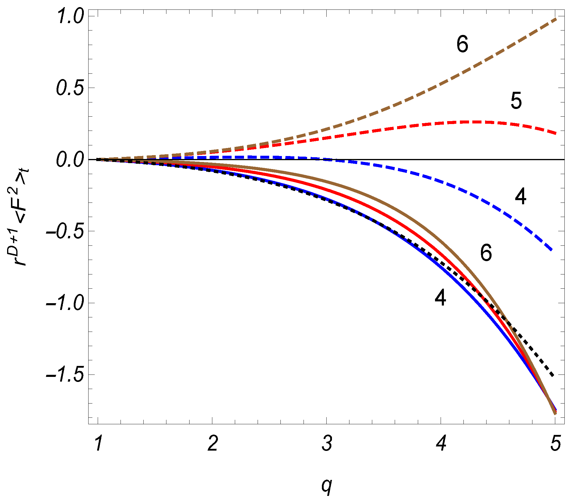
In $D=3$, the VEVs of the squared electric and magnetic fields coincide [9]. In Figure 2, we display the topological contributions in the VEVs of the squared electric and magnetic fields, multiplied by $r^{D+1}$, as functions of the parameter q for different values of the spatial dimension D (the numbers near the curves). The full and dashed curves correspond to the electric and magnetic fields, respectively, and the dotted curve presents the VEVs for $D=3$.

Having the VEVs of the squared electric and magnetic fields, we can evaluate the VEV of the Lagrangian density

$$\langle L\rangle =-\frac{1}{16\pi }{g}^{\mu \rho }{g}^{\nu \sigma }\langle F_{\mu \nu }{F}_{\rho \sigma }\rangle =\frac{\langle E^2\rangle -\langle B^2\rangle }{8\pi }.$$

(33)

The quantity $g^{\mu \rho }{g}^{\nu \sigma }\langle F_{\mu \nu }{F}_{\rho \sigma }\rangle$ is the Abelian analog of the gluon condensate in quantum chromodynamics (see, for instance, [27]). Note that, in a number of models (for example, string effective gravity [28,29] and models for generation of primordial magnetic fields during inflation [30]), the Lagrangian density contains terms of the form $f\left(\mathrm{\Phi }\right)F_{\mu \nu }{F}^{\mu \nu }$ that couple the gauge field to a scalar field $\mathrm{\Phi }$ (dilation field in string effective gravity and inflation in models of magnetic field generation). In these models, the appearance of the nonzero VEV $\langle F_{\mu \nu }{F}^{\mu \nu }\rangle$ induces a contribution to the effective potential for the field $\mathrm{\Phi }$. The stabilization of the dilation field during the cosmological expansion, based on the nontrivial coupling of dilation to other fields, has been discussed in [28]. By using Equations (21) and (30), for the topological contribution in the VEV of the Lagrangian density one gets

$${\langle L\rangle }_{\mathrm{t}}=-\frac{\left(D-3\right)\mathrm{\Gamma }(\left(D+1\right)/2)}{{\left(4\pi \right)}^{(D+1)/2}{r}^{D+1}}\left(D-1\right)c_{D-1}\left(q\right).$$

(34)

This VEV vanishes for $D=3$ and is negative for $D⩾4$.

The modification of the vacuum fluctuations for the electromagnetic field by a cosmic string gives rise to the Casimir–Polder forces acting on a neutral polarizable microparticle placed close to the string. For the general case of anisotropic polarizability the corresponding potential in the geometry of a $D=3$ cosmic string has been derived in [13]. For a special case of isotropic polarizability ${\alpha }_P\left(\omega \right)$, the corresponding formula takes the form

$$U\left(r\right)=\frac{r^{-4}}{8\pi }\left[\underset{l=1}{\overset{[q/2]}{{\sum }^{\prime }}}\frac{h(r,s_l)}{s_l^4}-\frac{q}{\pi }sin\left(q\pi \right){\int }_0^{\infty }dy\frac{h(r,coshy){cosh}^{-4}y}{cosh\left(2qy\right)-cos\left(q\pi \right)}\right],$$

(35)

with the function

$$h(r,y)={\int }_0^{\infty }dx{e}^{-x}{\alpha }_P(ix/\left(2ry\right))\left[y^2\left(1+x-x^2\right)+x^2\right].$$

(36)

If the dispersion of the polarizability can be neglected, one gets $h(r,y)=2{\alpha }_P$, with ${\alpha }_P$ being the static polarizability, and consequently

$$U\left(r\right)={\alpha }_P\frac{q^2-1}{360\pi r^4}\left(q^2+11\right).$$

(37)

For ${\alpha }_P>0$, the corresponding force is repulsive.

4. Energy–Momentum Tensor

Another important local characteristic of the vacuum state is the VEV of the energy–momentum tensor. It determines the back-reaction of quantum effects on the background geometry. The VEV is evaluated by using the formula

$$\langle T_{\mu }^{\nu }\rangle =-\frac{1}{4\pi }{C}_{\mu }^{\nu }-{\delta }_{\mu }^{\nu }\langle L\rangle ,$$

(38)

where

$$C_{\mu }^{\nu }=g^{\nu \kappa }{g}^{\rho \sigma }\sum _{\beta }{F}_{\left(\beta \right)\mu \rho }{F}_{\left(\beta \right)\kappa \sigma }^{*}.$$

(39)

By taking into account that $C_0^0=-\langle E^2\rangle$ and using Equation (34) for $\langle L\rangle$, for the topological part in the VEV of the energy density, one gets

$${\langle T_0^0\rangle }_{\mathrm{t}}=\frac{\mathrm{\Gamma }(\left(D+1\right)/2)}{{\left(4\pi \right)}^{(D+1)/2}{r}^{D+1}}\left[{\left(D-3\right)}^2{c}_{D-1}\left(q\right)-\left(D-1\right)c_{D+1}\left(q\right)\right].$$

(40)

Depending on the parameters q and D, the energy density (Equation (40)) can be either positive or negative.

For the components of Equation (39), corresponding to the axial stresses, one gets (no summation over $l=3,\dots ,D$)

$$C_l^l=-\frac{8\pi }{D-3}\langle L\rangle +\frac{4{\left(4\pi \right)}^{1-D/2}q}{\mathrm{\Gamma }\left(D/2\right)}\underset{m=0}{\overset{\infty }{{\sum }^{\prime }}}{\int }_0^{\infty }dk{k}^{D-1}{\int }_0^{\infty }d\gamma \frac{\gamma }{\omega }\left[G_{qm}\left(\gamma r\right)+\frac{D-3}{2}{J}_{qm}^2\left(\gamma r\right)\right].$$

(41)

The transformation of the second term in the right-hand side is done in a way similar to that for the squared electric field and for the axial stresses we find (no summation over l)

$${\langle T_l^l\rangle }_{\mathrm{t}}={\langle T_0^0\rangle }_{\mathrm{t}},l=3,\dots ,D.$$

(42)

This relation could also be directly obtained from the Lorentz invariance of the problem with respect to the boosts along the directions $z^l$, $l=3,\dots ,D$.

The off-diagonal components of the vacuum energy–momentum tensor vanish and it remains to consider the VEVs of the radial and azimuthal stresses. For the radial component of the tensor (Equation (39)), one finds

$$C_1^1=\frac{4{\left(4\pi \right)}^{1-D/2}q}{\mathrm{\Gamma }(D/2-1)}\underset{m=0}{\overset{\infty }{{\sum }^{\prime }}}\int dk{k}^{D-3}{\int }_0^{\infty }d\gamma \frac{{\gamma }^3}{\omega }\left[\left(D-1\right)J_{qm}^{\prime 2}\left(\gamma r\right)-G_{qm}\left(\gamma r\right)+J_{qm}^2\left(\gamma r\right)\right].$$

(43)

The evaluation of the parts corresponding to the last two terms in the square brackets in Equation (43) is similar to that for the corresponding parts on the squared electric field. For the remaining part, by using Equation (11), we get

$${\int }_0^{\infty }dk{k}^{D-3}{\int }_0^{\infty }d\gamma \frac{{\gamma }^3}{\omega }{J}_{qm}^{\prime 2}\left(\gamma r\right)=\frac{\mathrm{\Gamma }(D/2-1)}{\sqrt{\pi }}{\int }_0^{\infty }\frac{dy}{y^{D-2}}{\int }_0^{\infty }d\gamma {\gamma }^3{e}^{-{\gamma }^2{y}^2}{J}_{qm}^{\prime 2}\left(\gamma r\right).$$

(44)

The integral is evaluated by using the relation

$${\int }_0^{\infty }d\gamma {\gamma }^3{e}^{-{\gamma }^2{y}^2}{J}_{qm}^{\prime 2}\left(\gamma r\right)=\underset{r\to r^{\prime }}{lim}{\partial }_r{\partial }_{r^{\prime }}{\int }_0^{\infty }d\gamma \gamma e^{-{\gamma }^2{y}^2}{J}_{qm}\left(\gamma r\right)J_{qm}\left(\gamma r^{\prime }\right),$$

(45)

and Equation (13). The further steps are similar to that for the VEVs of the squared fields and are based on Equation (18). In this way, one finds

$${\langle T_1^1\rangle }_{\mathrm{t}}=-\frac{\mathrm{\Gamma }\left((D+1)/2\right)}{{\left(4\pi \right)}^{(D+1)/2}{r}^{D+1}}\left(D-1\right)c_{D+1}\left(q\right).$$

(46)

Finally, for the component $C_2^2$, one has

$$C_2^2=\frac{4{\left(4\pi \right)}^{D/2-1}q}{\mathrm{\Gamma }(D/2-1)}\underset{m=0}{\overset{\infty }{{\sum }^{\prime }}}\int d\mathbf{k}{\int }_0^{\infty }d\gamma \frac{{\gamma }^3}{\omega }\left[\left(1-D\right)J_{qm}^{\prime 2}\left(x\right)+\left(D-2\right)G_{qm}\left(\gamma r\right)+J_{qm}^{\prime 2}\left(x\right)\right],$$

(47)

and the evaluation is similar to that for Equation (43). For the azimuthal stress, one gets

$${\langle T_2^2\rangle }_{\mathrm{t}}=\frac{\mathrm{\Gamma }\left((D+1)/2\right)}{{\left(4\pi \right)}^{(D+1)/2}{r}^{D+1}}D\left(D-1\right)c_{D+1}\left(q\right).$$

(48)

As seen, one has the relation ${\langle T_2^2\rangle }_{\mathrm{t}}=-D{\langle T_1^1\rangle }_{\mathrm{t}}$. The VEV of the energy–momentum tensor obeys the covariant conservation equation ${\nabla }_{\nu }{\langle T_{\mu }^{\nu }\rangle }_{\mathrm{t}}=0$. For the geometry under consideration the latter is reduced to the single equation ${\partial }_r\left(r{\langle T_1^1\rangle }_{\mathrm{t}}\right)={\langle T_2^2\rangle }_{\mathrm{t}}$. For $D=3$, the vacuum energy–momentum tensor is traceless, ${\langle T_{\mu }^{\mu }\rangle }_{\mathrm{t}}=0$. For $D\ne 3$, the electromagnetic field is not conformally invariant and the trace is not zero.

For $D=3$, by taking into account Equation (24), one finds

$${\langle T_{\mu }^{\nu }\rangle }_{\mathrm{t}}=-\frac{q^2-1}{720{\pi }^2{r}^4}\left(q^2+11\right)\mathrm{diag}\left(1,1,-3,1\right).$$

(49)

In particular, the energy density is negative for $q>1$. This result was obtained in [6,7] by using the corresponding Green function. In the special case $D=5$, we have (no summation over l)

$${\langle T_l^l\rangle }_{\mathrm{t}}=-\frac{\left(q^2-1\right)\left(q^2+5\right)\left(q^2-4\right)}{945{\left(2\pi \right)}^3{r}^6},$$

(50)

for $l=0,3,\dots ,D$, and

$${\langle T_1^1\rangle }_{\mathrm{t}}=-\frac{1}{5}{\langle T_2^2\rangle }_{\mathrm{t}}=-\frac{q^2-1}{1890{\left(2\pi \right)}^3{r}^6}(2q^4+23q^2+191).$$

(51)

The energy density is positive for $1<q<2$ and negative for $q>2$. In the special case $q=2$, and for general D, one obtains

$${\langle T_{\mu }^{\nu }\rangle }_{\mathrm{t}}=\frac{\left(D-2\right)\mathrm{\Gamma }(\left(D+1\right)/2)}{2{\left(4\pi \right)}^{(D+1)/2}{r}^{D+1}}\mathrm{diag}\left(D-5,-\frac{D-1}{D-2},D\frac{D-1}{D-2},D-5,\dots ,D-5\right).$$

(52)

The corresponding energy density vanishes for $D=5$.

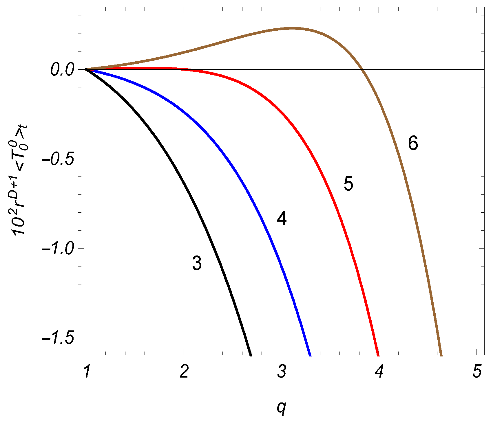
In Figure 3, we plot the VEV of the energy density, multiplied by $r^{D+1}$, versus the parameter q for different values of the spatial dimension D (the numbers near the curves). For $D⩾5$, the energy density is positive for small values of q and is negative for large values of that parameter. For some intermediate value of q there is a maximum with positive energy density.

5. VEVs for Cosmic String on Locally dS Bulk

In the second part of the paper, we consider the combined effects of a cosmic string and of the background gravitational field, generated by a positive cosmological constant, on the VEVs of the squared electric and magnetic fields and on the vacuum energy density. This investigation has been recently presented in [16] based on the corresponding two-point functions for the electromagnetic field tensor. Here, we follow a simpler approach based on the direct evaluation of the mode sums introducing a cutoff function. The vacuum polarization induced by a cosmic string in locally (but not globally) dS spacetime for massive scalar and fermionic fields has been investigated in [31,32,33].

Our choice of the locally dS geometry is motivated by several reasons. First, the dS spacetime is maximally symmetric and similar to case of the flat bulk the problem for evaluation of the local characteristics of the electromagnetic field is exactly solvable. In addition, the dS spacetime plays an important role in modern cosmology. In most inflationary models, the early expansion of the universe is quasi de Sitterian (for the effects of inflation on the cosmic strings, see [34,35,36,37]). The corresponding accelerated expansion before the radiation dominated era naturally solves a number of problems in the standard cosmological model. The inflation also provides an attractive mechanism of producing long-wavelength electromagnetic fluctuations, originating from subhorizon-sized quantum fluctuations of the electromagnetic field stretched by the dS phase to superhorizon scales. In the post-inflationary era, these long-wavelength fluctuations re-enter the horizon and can serve as seeds for cosmological magnetic fields. Related to this mechanism, the cosmological dynamics of the electromagnetic field quantum fluctuations have been discussed in large number of papers (see [38,39,40] and references therein). More recently, the observational data on high redshift supernovae, galaxy clusters, and cosmic microwave background indicate that at the present epoch the universe is accelerating and the corresponding expansion is driven by a source the properties of which are close to a positive cosmological constant. In this case, the quasi-dS geometry is the future attractor for the universe. Though the cosmic strings produced before or during early stages of the inflationary phase are diluted by the quasi-exponential expansion, the defects can be formed near or at the end of inflation by several mechanisms (see [2] for possible observational consequences from this type of models). It is also possible to have subsequent inflationary stages, with linear defects being formed in between them [41].

5.1. Electromagnetic Field Modes

In terms of the conformal time coordinate $\tau$, $-\infty <\tau <0$, the line element describing the geometry under consideration is given by the expression

$$d{s}^2={\left(\alpha /\tau \right)}^2[d{\tau }^2-d{r}^2-r^{2}d{\varphi }^2-{\left(d\mathbf{z}\right)}^2],$$

(53)

where the ranges for the spatial coordinates are the same as in Equation (1). In the absence of cosmic string one has ${\varphi }_0=2\pi$ and the geometry coincides with the dS one in inflationary coordinates. For the synchronous time t, one has $t=-\alpha ln(\left|\tau \right|/\alpha ),-\infty <t<+\infty$. The parameter $\alpha$ is related to the cosmological constant $\mathrm{\Lambda }$ by $\mathrm{\Lambda }=D(D-1)/\left(2{\alpha }^2\right)$. It has been argued in [42,43] that the vortex solution of the Einstein–Abelian–Higgs equations in the presence of a cosmological constant induces a deficit angle into dS spacetime. Similar to the case of the dS spacetime, we can also write the line element (Equation (53)) with an angular deficit in static coordinates. For simplicity, considering the case $D=4$, the corresponding transformation reads

$$t=t_s-\alpha lnf\left(r_s\right),r=r_{s}f\left(r_s\right)e^{-t_s/\alpha }sin\theta ,z_1=r_{s}f\left(r_s\right)e^{-t_s/\alpha }cos\theta ,\varphi =\varphi ,$$

(54)

where $f\left(r_s\right)=1/\sqrt{1-r_s^2/{\alpha }^2}$. The line element takes the form

$$d{s}^2=f^{-2}\left(r_s\right)d{t}_s^2-f^2\left(r_s\right)d{r}_s^2-r_s^2(d{\theta }^2+{sin}^2\theta d{\varphi }^2),$$

(55)

with $0\le \varphi \le {\varphi }_0$. With a new coordinate $\phi =q\varphi$, from Equation (55), we obtain the static line element of dS spacetime with deficit angle previously discussed in [42]. In this paper, it is shown that to leading order in the gravitational coupling the effect of the vortex on dS spacetime is to create a deficit angle in the metric (Equation (55)).

For the coordinates corresponding to Equation (53) and for the Bunch–Davies vacuum state, the cylindrical electromagnetic modes are presented as

$$\begin{array}{ccc}\hfill A_{\left(\beta \right)\mu }\left(x\right)& =& c_{\beta }{\eta }^{\frac{D}{2}-1}{H}_{\frac{D}{2}-1}^{\left(1\right)}\left(\omega \eta \right)\left(0,\frac{iqm}{r},-r{\partial }_r,0,\dots ,0\right)J_{q\left|m\right|}\left(\gamma r\right)e^{iqm\varphi +i\mathbf{k}·\mathbf{z}},\sigma =1,\hfill \\ \hfill A_{\left(\beta \right)\mu }\left(x\right)& =& c_{\beta }\omega {\eta }^{\frac{D}{2}-1}{H}_{\frac{D}{2}-1}^{\left(1\right)}\left(\omega \eta \right)\left(0,{ϵ}_{\sigma l}+i\frac{\mathbf{k}·{\mathit{ϵ}}_{\sigma }}{{\omega }^2}{\partial }_l\right)J_{q\left|m\right|}\left(\gamma r\right)e^{iqm\varphi +i\mathbf{k}·\mathbf{z}},\sigma =2,\dots ,D-1,\hfill \end{array}$$

(56)

where $H_{\nu }^{\left(1\right)}\left(x\right)$ is the Hankel function of the first kind and $\eta =\left|\tau \right|$. Other notations in Equation (56) are the same as in Equation (2). For the normalization constant from Equation (4), one finds

$$|c_{\beta }{|}^2=\frac{q}{4{\left(2\pi \alpha \right)}^{D-3}\gamma }.$$

(57)

For $D=3$, the electromagnetic field is conformally invariant and the modes in Equation (56) coincide with Equation (2).

5.2. Squared Electric Field

We start with the VEV of the squared electric field obtained from Equation (8). The VEV, regularized by introducing the cutoff function $e^{-b{\omega }^2}$, is presented as

$$\begin{array}{ccc}\hfill {\langle E^2\rangle }_{\mathrm{reg}}& =& \frac{2^{5-D}q{\eta }^{D+2}}{{\pi }^{D/2}\mathrm{\Gamma }(D/2-1){\alpha }^{D+1}}\underset{m=0}{\overset{\infty }{{\sum }^{\prime }}}{\int }_0^{\infty }dk{k}^{D-3}{\int }_0^{\infty }d\gamma \gamma {\left|K_{\nu }\left(e^{i\pi /2}\omega \eta \right)\right|}^2\hfill \\ & & \times e^{-b{\omega }^2}\left\{\left[(D-2){\gamma }^2+(D-3)k^2\right]J_{qm}^{\prime 2}\left(\gamma r\right)+\left({\gamma }^2+2k^2\right)G_{qm}\left(\gamma r\right)\right\},\hfill \end{array}$$

(58)

where we have introduced the MacDonald function $K_{\nu }\left(x\right)$ instead of the Hankel function, $\nu =D/2-2$ and the other notations are the same as in Equation (9). For the further transformation, we use the integral representation

$${|K_{\nu }\left(e^{i\pi /2}\eta \omega \right)|}^2=\frac{1}{2}{\int }_0^{\infty }dycosh\left(\nu y\right){\int }_0^{\infty }\frac{dx}{x}{e}^{-2{\eta }^2\left(coshy-1\right)/x-x{\omega }^2/4}.$$

(59)

This relation is obtained from the integral representation of the product of MacDonald functions with different arguments given in [44]. Plugging Equation (59) into Equation (58), the integration over k is elementary and the integral over y is expressed in terms of the function $K_{\nu }(2{\eta }^2/x)$. In this way, one gets

$$\begin{array}{ccc}\hfill {\langle E^2\rangle }_{\mathrm{reg}}& =& \frac{8q{\eta }^{D+2}}{{\left(4\pi \right)}^{D/2}{\alpha }^{D+1}}\underset{m=0}{\overset{\infty }{{\sum }^{\prime }}}{\int }_0^{\infty }dx\frac{e^{2{\eta }^2/x}}{x{w}^{D/2}}{K}_{\nu }(2{\eta }^2/x){\int }_0^{\infty }d\gamma \gamma \hfill \\ & & \times \left[\left(D-2+w{\partial }_w\right)G_{qm}\left(\gamma r\right)+(D-2)\left(\frac{D-3}{2}-w{\partial }_w\right)J_{qm}^{\prime 2}\left(\gamma r\right)\right]e^{-w{\gamma }^2},\hfill \end{array}$$

(60)

where $w=x/4+b$. The integrals over $\gamma$ are evaluated by using Equations (13) and (16), and we find

$$\begin{array}{ccc}\hfill {\langle E^2\rangle }_{\mathrm{reg}}& =& \frac{8q{(\eta /r)}^{D+2}}{{\left(2\pi \right)}^{D/2}{\alpha }^{D+1}}{\int }_0^{\infty }\frac{dx}{x}{e}^{2{\eta }^2/x}{K}_{D/2-2}(2{\eta }^2/x)u^{D/2+1}\hfill \\ & & \times \left[\left(D-2+{\partial }_{u}u\right)\left({\partial }_u+1\right)+(D-2)\left(\frac{D-3}{2}+{\partial }_{u}u\right)\right]e^{-u}\underset{m=0}{\overset{\infty }{{\sum }^{\prime }}}{I}_{qm}\left(u\right),\hfill \end{array}$$

(61)

with $u=r^2/\left[2\left(x/4+b\right)\right]$.

Next, we use Equation (18) for the series over m. The $l=0$ term gives the regularized VEV in dS spacetime in the absence of the cosmic string, denoted here as ${\langle E^2\rangle }_{\mathrm{dS}}^{\mathrm{reg}}$. The remaining part corresponds to the contribution of the cosmic string. For points $r\ne 0$ that part is finite in the limit $b\to 0$ and the cutoff can be removed. In this way, for the topological part ${\langle E^2\rangle }_{\mathrm{t}}=\langle E^2\rangle -{\langle E^2\rangle }_{\mathrm{dS}}$, one gets [16]

$${\langle E^2\rangle }_{\mathrm{t}}=\frac{8{\alpha }^{-D-1}}{{\left(2\pi \right)}^{D/2}}\left[\underset{l=1}{\overset{[q/2]}{{\sum }^{\prime }}}{g}_E(r/\eta ,s_l)-\frac{q}{\pi }sin\left(q\pi \right){\int }_0^{\infty }dy\frac{g_E(r/\eta ,coshy)}{cosh\left(2qy\right)-cos\left(q\pi \right)}\right],$$

(62)

where ${\langle E^2\rangle }_{\mathrm{dS}}$ is the renormalized VEV in the absence of the cosmic string. In Equation (62), we have introduced the notation $s_l=sin(\pi l/q)$ and

$$g_E(x,y)={\int }_0^{\infty }du{u}^{D/2}{K}_{D/2-2}\left(u\right)e^{u-2x^2{y}^{2}u}\left[2u{x}^2{y}^2\left(2y^2-D+1\right)+\left(D-1\right)\left(D/2-2y^2\right)\right].$$

(63)

Note that the regularized VEV for dS bulk in the absence of cosmic string has the form

$${\langle E^2\rangle }_{\mathrm{dS}}^{\mathrm{reg}}=\frac{2D\left(D-1\right)}{{\left(2\pi \right)}^{D/2}{\alpha }^{D+1}}{\int }_0^{\infty }dz\frac{z^{D/2}{e}^z{K}_{D/2-2}\left(z\right)}{{\left(1+2zb/{\eta }^2\right)}^{D/2+1}}.$$

(64)

As expected, this VEV diverges in the limit $b\to 0$ and requires a renormalization. From the maximal symmetry of dS spacetime and of the Bunch–Davies vacuum state, we expect that the renormalized VEV does not depend on the spacetime point and ${\langle E^2\rangle }_{\mathrm{dS}}=\mathrm{const}·{\alpha }^{-D-1}$. In Equation (62), the topological part depends on the coordinates r and $\eta$ in the form of the ratio $r/\eta$. The latter is the proper distance from the string, $\alpha r/\eta$, measured in units of the dS curvature scale $\alpha$.

For odd values of D, the function $g_E(x,y)$ in Equation (62) is expressed in terms of the elementary functions. In particular, one finds

$$\begin{array}{ccc}\hfill {\langle E^2\rangle }_{\mathrm{t}}& =& -\frac{\left(q^2-1\right)\left(q^2+11\right)}{180\pi {(\alpha r/\eta )}^4},D=3,\hfill \\ \hfill {\langle E^2\rangle }_{\mathrm{t}}& =& -\frac{\left(q^2-1\right)\left(q^4+22q^2+211\right)}{1890{\pi }^2{\left(\alpha r/\eta \right)}^6},D=5.\hfill \end{array}$$

(65)

For $D=3$, the electromagnetic field is conformally invariant and the topological contribution is related to the one for the flat bulk by standard conformal relation. It is of interest to note that a similar relation takes place for $D=5$ as well. For other values of D, there is no such a simple relation.

For points near the string, assuming that $r/\eta \ll 1$, the contribution of the large u is dominant in Equation (63). By using the corresponding asymptotic expression for the MacDonald function, to the leading order, we get ${\langle E^2\rangle }_{\mathrm{t}}\approx {(\eta /\alpha )}^{D+1}{\langle E^2\rangle }_{\mathrm{t}}^{\left(\mathrm{M}\right)}$, where ${\langle E^2\rangle }_{\mathrm{t}}^{\left(\mathrm{M}\right)}$ is topological contribution in the flat bulk and is given by Equation (21). Near the string, the main contribution to the VEVs comes from the fluctuations with wavelengths smaller than the curvature radius and the influence of the background gravitational field on the corresponding modes is weak.

At proper distances from the string larger than the dS curvature radius one has $r/\eta \gg 1$. Now, the contribution from the region near the lower limit of the integration in Equation (63) is dominant. For $D⩾5$, to the leading order, the topological part is expressed in terms of $c_4\left(q\right)$ and $c_6\left(q\right)$:

$${\langle E^2\rangle }_{\mathrm{t}}\approx \frac{\mathrm{\Gamma }\left(D/2-2\right)\left(q^2-1\right)}{8{\pi }^{D/2}{\alpha }^{D+1}{\left(r/\eta \right)}^6}\left[\frac{D-1}{21}\left(D-6\right)(2q^4+23q^2+191)-4\left(D-4\right)\left(q^2+11\right)\right].$$

(66)

In the special case, $D=4$ from Equation (62), we get

$${\langle E^2\rangle }_{\mathrm{t}}\approx -\frac{\left(q^2-1\right)ln(r/\eta )}{630{\pi }^2{\alpha }^5{(r/\eta )}^6}(2q^4+23q^2+191).$$

(67)

For $D=3$, one has the behavior given by Equation (65). At large distances, the total VEV is dominated by the part ${\langle E^2\rangle }_{\mathrm{dS}}$. As seen, in spatial dimensions $D=4,6,7,\dots$, at distances larger than the curvature radius, the influence of the gravitational field on the topological part is essential. From Equations (66) and (67), it follows that at large distances ${\langle E^2\rangle }_{\mathrm{t}}<0$ for $D=4,5,6$, and ${\langle E^2\rangle }_{\mathrm{t}}>0$ for $D⩾7$. By taking into account that near the string one has ${\langle E^2\rangle }_{\mathrm{t}}<0$ for $D⩾3$, we conclude that in spatial dimensions $D⩾7$ the topological contribution ${\langle E^2\rangle }_{\mathrm{t}}$ has a positive maximum for some intermediate value of $r/\eta$.

5.3. Squared Magnetic Field

By using the mode functions (Equation (56)), from the mode-sum formula (Equation (27)), one gets the following representation for the squared magnetic field

$$\begin{array}{ccc}\hfill {\langle B^2\rangle }_{\mathrm{reg}}& =& \frac{2^{5-D}{\pi }^{-D/2}q{\eta }^{D+2}}{\mathrm{\Gamma }(D/2-1){\alpha }^{D+1}}\underset{m=0}{\overset{\infty }{{\sum }^{\prime }}}{\int }_0^{\infty }dk{k}^{D-3}{\int }_0^{\infty }d\gamma \gamma K_{D/2-1}\left(e^{-i\pi /2}\omega \eta \right)K_{D/2-1}\left(e^{i\pi /2}\omega \eta \right)\hfill \\ & & \times e^{-b{\omega }^2}\left\{\left[\left(D-2\right){\gamma }^2+2k^2\right]G_{qm}\left(\gamma r\right)+\left[{\gamma }^2+(D-3)k^2\right]J_{qm}^{\prime 2}\left(\gamma r\right)\right\}.\hfill \end{array}$$

(68)

Further transformation of this VEV is similar to that for the electric field squared. The final formula for the topological contribution ${\langle B^2\rangle }_{\mathrm{t}}=\langle B^2\rangle -{\langle B^2\rangle }_{\mathrm{dS}}$ is given by [16]

$${\langle B^2\rangle }_{\mathrm{t}}=\frac{8{\alpha }^{-D-1}}{{\left(2\pi \right)}^{D/2}}\left[\underset{l=1}{\overset{[q/2]}{{\sum }^{\prime }}}{g}_M(r/\eta ,s_l)-\frac{q}{\pi }sin\left(q\pi \right){\int }_0^{\infty }dy\frac{g_M(r/\eta ,coshy)}{cosh\left(2qy\right)-cos\left(q\pi \right)}\right],$$

(69)

with the function

$$\begin{array}{ccc}\hfill g_M(x,y)& =& {\int }_0^{\infty }du{u}^{D/2}{K}_{D/2-1}\left(u\right)e^{u-2x^2{y}^{2}u}\left\{(D-1)D/2\right.\hfill \\ & & \left.-4(D-2)y^2+2x^2{y}^{2}u\left[2(D-2)y^2-D+1\right]\right\}.\hfill \end{array}$$

(70)

We denote by ${\langle B^2\rangle }_{\mathrm{dS}}$ the renormalized VEV of the squared magnetic field in dS spacetime in the absence of the cosmic string. The regularized VEV of the squared magnetic field for the latter geometry is given by

$${\langle B^2\rangle }_{\mathrm{dS}}^{\mathrm{reg}}=\frac{2D\left(D-1\right)}{{\left(2\pi \right)}^{D/2}{\alpha }^{D+1}}{\int }_0^{\infty }dz\frac{z^{D/2}{e}^z{K}_{D/2-1}\left(z\right)}{{\left(1+2zb/{\eta }^2\right)}^{D/2+1}}.$$

(71)

For $D=3$, this result coincides with that for the squared electric field. Note that, for $D=4$ and $q=3$, the topological part vanishes, ${\langle B^2\rangle }_{\mathrm{t}}=0$.

For odd values of the spatial dimension D the integral in Equation (70) is expressed in terms of the elementary functions. For $D=3$, one has ${\langle B^2\rangle }_{\mathrm{t}}={\langle E^2\rangle }_{\mathrm{t}}$ and, for $D=5$, we get

$${\langle B^2\rangle }_{\mathrm{t}}=\frac{\left(3+r^2/{\eta }^2\right)c_4\left(q\right)-c_6\left(q\right)}{2{\pi }^2{\left(\alpha r/\eta \right)}^6}.$$

(72)

Note that, unlike to the case of the electric field, the VEV of the squared magnetic field for $D=5$ does not coincide with the corresponding VEV in flat bulk with the distance r replaced by the proper distance $\alpha r/\eta$.

For points near the string, $r/\eta \ll 1$, the influence of the gravitational field on the topological contribution is weak and to the leading order one has the relation ${\langle B^2\rangle }_{\mathrm{t}}\approx {\left(\eta /\alpha \right)}^{D+1}{\langle B^2\rangle }_{\mathrm{t}}^{\left(\mathrm{M}\right)}$, where the VEV ${\langle B^2\rangle }_{\mathrm{t}}^{\left(\mathrm{M}\right)}$ is given by Equation (30). The influence of the gravitational field is essential at proper distances from the string larger than the curvature radius of dS spacetime. In the asymptotic region $r/\eta \gg 1$, for the leading terms in the expansions of the topological parts, one has

$$\begin{array}{ccc}\hfill {\langle B^2\rangle }_{\mathrm{t}}& \approx & -\frac{\left(q^2-1\right)\left(q^2-9\right)\left(2q^2+13\right)}{1260{\pi }^2{\alpha }^5{\left(r/\eta \right)}^6},D=4,\hfill \\ \hfill {\langle B^2\rangle }_{\mathrm{t}}& \approx & \frac{(D-1)\left(D-4\right)\mathrm{\Gamma }(D/2-1)}{4{\pi }^{D/2}{\alpha }^{D+1}{(r/\eta )}^4}{c}_4\left(q\right),D\ne 4.\hfill \end{array}$$

(73)

Note that, for $D=4$, at large distances, one has ${\langle E^2\rangle }_{\mathrm{t}}/{\langle B^2\rangle }_{\mathrm{t}}\propto ln(r/\eta )$, whereas, for $D⩾5$, one has ${\langle E^2\rangle }_{\mathrm{t}}/{\langle B^2\rangle }_{\mathrm{t}}\propto {(r/\eta )}^{-2}$ and the topological part in the VEV of the squared magnetic field is much larger than the one for the electric field. For $D⩾5$ the topological part ${\langle B^2\rangle }_{\mathrm{t}}$ is positive at large distances.

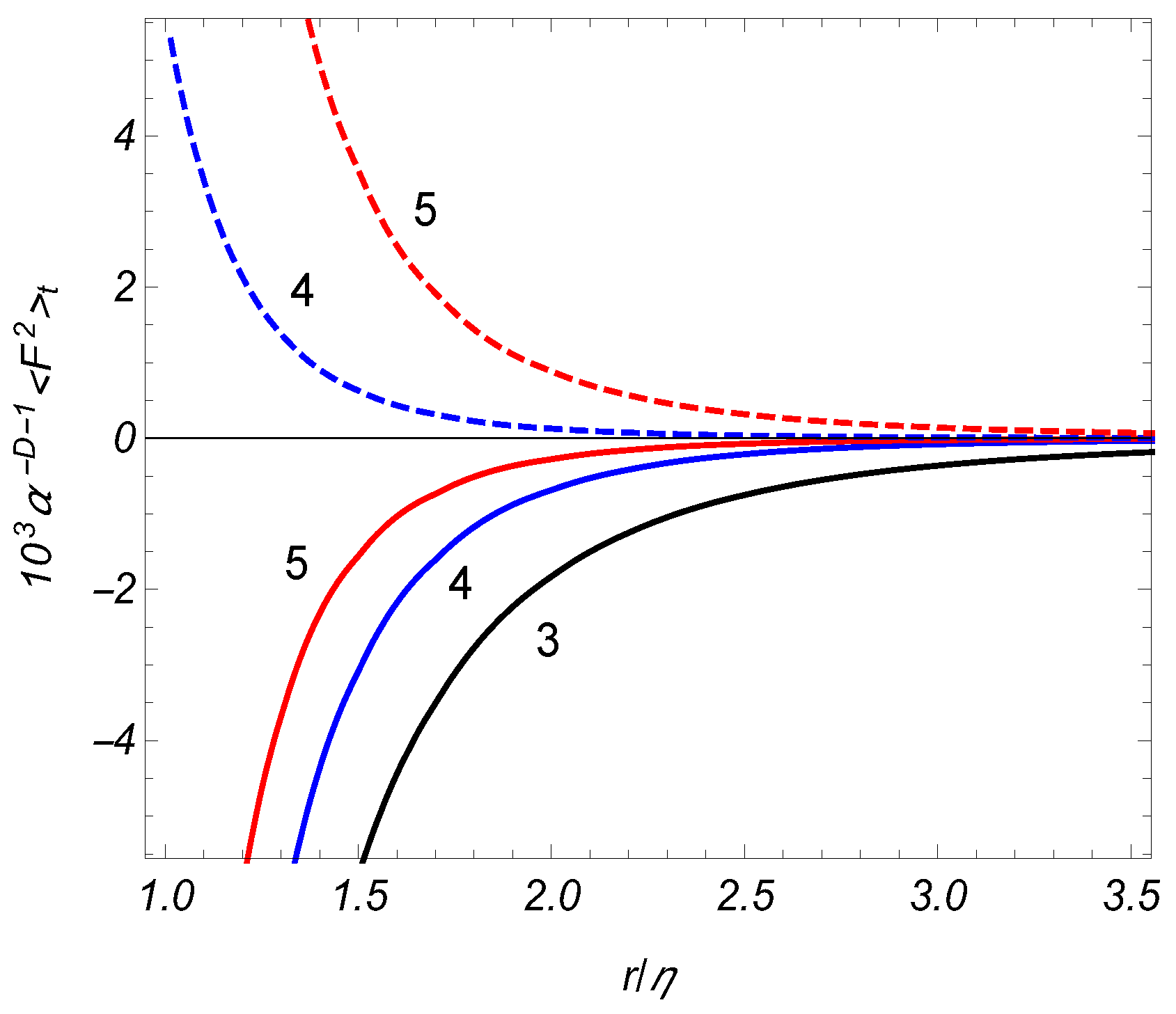
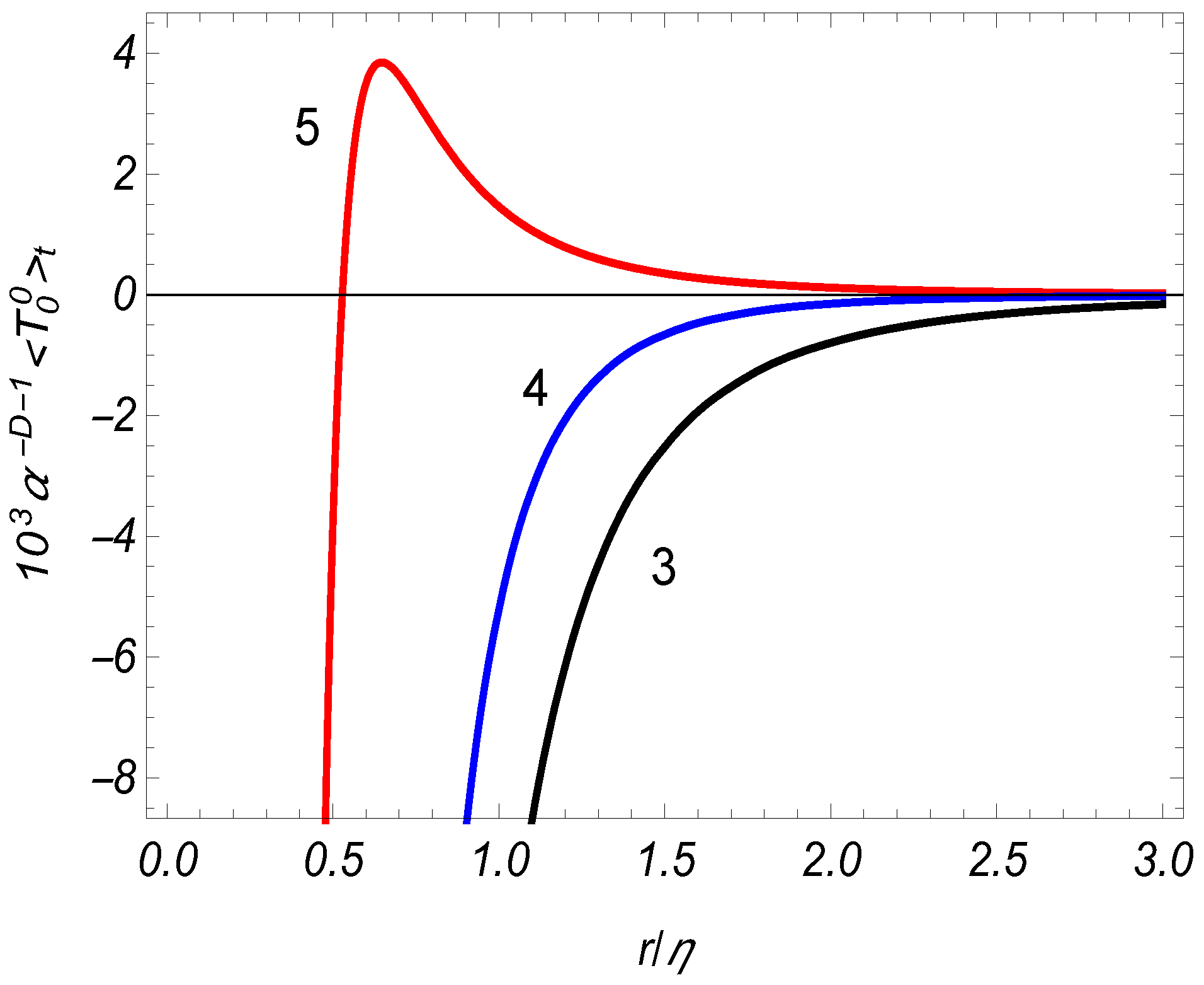
In Figure 4, we have displayed the dependence of the VEVs for squared electric (full curves) and magnetic (dashed curves) fields on the ratio $r/\eta$ (proper distance from the string in units of the dS curvature scale $\alpha$) for separate values of the spatial dimension $D=3,4,5$. For $D=3$, the VEVs for the electric and magnetic fields coincide. The graphs are plotted for $q=1.5$.

5.4. VEV of the Energy Density

The VEV of the energy density is given by $\langle T_0^0\rangle =\left(\langle E^2\rangle +\langle B^2\rangle \right)/8\pi$ and is decomposed as $\langle T_0^0\rangle ={\langle T_0^0\rangle }_{\mathrm{dS}}+{\langle T_0^0\rangle }_{\mathrm{t}}$, where ${\langle T_{\mu }^{\nu }\rangle }_{\mathrm{dS}}=\mathrm{const}·{\delta }_{\mu }^{\nu }$ is the VEV in dS spacetime in the absence of the cosmic string. For the topological contribution, one gets the expression

$${\langle T_0^0\rangle }_{\mathrm{t}}=\frac{2{\alpha }^{-D-1}}{{\left(2\pi \right)}^{D/2+1}}\left[\underset{l=1}{\overset{[q/2]}{{\sum }^{\prime }}}g(r/\eta ,s_l)-\frac{q}{\pi }sin\left(q\pi \right){\int }_0^{\infty }dy\frac{g(r/\eta ,coshy)}{cosh\left(2qy\right)-cos\left(q\pi \right)}\right],$$

(74)

with the function

$$\begin{array}{ccc}\hfill g(x,y)& =& {\int }_0^{\infty }du{u}^{D/2}{e}^{u-2x^2{y}^{2}u}\left\{K_{\frac{D}{2}-2}\left(u\right)\left[\left(D-1\right)\left(\frac{D}{2}-2y^2\right)+2x^2{y}^{2}u\left(2y^2-D+1\right)\right]\right.\hfill \\ & & \left.+K_{\frac{D}{2}-1}\left(u\right)\left[(D-1)\frac{D}{2}-4(D-2)y^2+2x^2{y}^{2}u\left(2(D-2)y^2-D+1\right)\right]\right\}.\hfill \end{array}$$

(75)

Near the string, $r/\eta \ll 1$, to the leading order, one has ${\langle T_0^0\rangle }_{\mathrm{t}}\approx {(\eta /\alpha )}^{D+1}{\langle T_0^0\rangle }_{\mathrm{t}}^{\left(\mathrm{M}\right)}$ with the energy density in flat bulk from (Equation (40)). At large distances from the string, one has the asymptotic expressions

$$\begin{array}{ccc}\hfill {\langle T_0^0\rangle }_{\mathrm{t}}& \approx & -\frac{\left(q^2-1\right)ln(r/\eta )}{5040{\pi }^3{\alpha }^5{(r/\eta )}^6}(2q^4+23q^2+191),D=4,\hfill \\ \hfill {\langle T_0^0\rangle }_{\mathrm{t}}& \approx & \frac{(D-1)\left(D-4\right)\mathrm{\Gamma }(D/2-1)}{2880{\pi }^{D/2+1}{\alpha }^{D+1}{(r/\eta )}^4}\left(q^2-1\right)\left(q^2+11\right),D⩾5.\hfill \end{array}$$

(76)

In this asymptotic region, the vacuum energy density is dominated by the part ${\langle T_0^0\rangle }_{\mathrm{dS}}$. The topological contribution is negative for $D=4$ and positive for $D⩾5$.

Figure 5 presents the energy density versus $r/\eta$ for different values of the spatial dimension $D=3,4,5$.

One of the interesting effects during the dS expansion, playing an important role in inflationary cosmology, is the so-called classicalization of quantum fluctuations: the evolution of quantum fluctuations into classical fluctuations. In particular, the latter for the inflation field are expected to be the seeds of large scale structures in the universe. In a similar way, the classicalization of the electromagnetic fluctuations may give rise to large scale magnetic fields (for various types of mechanisms for the generation of cosmological magnetic fields, see, for instance, [30,38,39,40]). The discussion we have presented above shows that these fields will be influenced by cosmic strings formed at late stages of the inflationary phase.

6. Conclusions

We have investigated the influence of a straight cosmic string on the local characteristics of the electromagnetic vacuum. First, we have considered a cosmic string on flat spacetime and then the corresponding results are generalized for the locally dS background geometry. A simplified model is used where the effect of the cosmic string on the background geometry is reduced to the generation of a planar angle deficit. In this model, for points outside the core, the local geometry is not changed by the cosmic string, but the global properties are different. The corresponding nontrivial topology gives rise to shifts in the VEVs of physical observables. For the investigation of the topological contributions, we have employed the direct summation over the complete set of electromagnetic modes.

For a cosmic string on $(D+1)$-dimensional flat spacetime the complete set of modes for the vector potential is given by Equation (2), where $\sigma$ enumerates the polarization states. For the regularization of the mode sums in the VEVs of squared electric and magnetic fields, the cutoff function $e^{-b{\omega }^2}$ is introduced. The application of Equation (18) for the summation over the azimuthal quantum number allowed us to extract explicitly the parts in the VEVs corresponding to the Minkwoski spacetime in the absence of the cosmic string. For points away from the string core, the remaining topological contributions are finite in the limit $b\to 0$ and the cutoff can be safely removed. These contributions for the electric and magnetic fields are given by Equations (21) and (30), where the function $c_n\left(q\right)$, depending on the planar angle deficit, is defined by Equation (22). In spatial dimensions $D⩾3$, the topological part in the VEV of the squared electric field is negative whereas, depending on q and D, the corresponding part for the magnetic field can be either negative or positive. For odd values of D, the functions $c_n\left(q\right)$ in the expressions for the topological contributions are polynomials in q and the VEVs are further simplified. In the special case $D=3$, the electromagnetic field is conformally invariant and the topological contributions for the electric and magnetic fields coincide.

Another important characteristic of the vacuum state that determines the back-reaction of quantum effects on the background geometry is the VEV of the energy–momentum tensor. For a cosmic string on flat bulk this VEV is diagonal. Due to the Lorentz invariance with respect to the boosts along directions $z^l$, $l=3,\dots ,D$, the topological contributions in the corresponding stresses coincide with the energy density, given by Equation (40). The radial and azimuthal stresses are given by Equations (46) and (48). They are related by a simple relation ${\langle T_2^2\rangle }_{\mathrm{t}}=-D{\langle T_1^1\rangle }_{\mathrm{t}}$ that is a direct consequence of the covariant conservation equation for the VEV of the energy–momentum tensor. The general expressions are simplified for an odd number of spatial dimension. In particular, for $D=3,5$, one gets the representations in Equations (49)–(51). Depending on the planar angle deficit and the spatial dimension, the corresponding energy density can be either negative or positive.

For a string in locally dS spacetime the electromagnetic mode functions, realizing the Bunch–Davies vacuum state, are presented as Equation (56). The topological contributions in the VEVs of the squared electric and magnetic fields are given by Equations (62) and (69) with the functions in Equations (63) and (70). The corresponding energy density is obtained by summing the contributions of the electric and magnetic parts. For points near the string, the dominant contribution to the VEVs come from the fluctuations with small wavelengths and the influence of the gravitational field is weak. In this region, the leading terms in the VEVs coincide with those for flat spacetime with the distance from the string replaced by the proper distance. The influence of the gravitational field is essential at proper distances larger than the curvature radius of dS spacetime. For $D=4$, the topological contributions in the VEVs decay as ${(r/\eta )}^{-6}ln(r/\eta )$ for the squared electric field and like ${(r/\eta )}^{-6}$ for the squared magnetic field. In this case, the corresponding energy density is dominated by the electrical part and is negative. For $D>4$, the topological contributions decay as ${(r/\eta )}^{-6}$ in the case of the electric field squared and as ${(r/\eta )}^{-4}$ for the magnetic field squared. The topological term in the vacuum energy density is dominated by the magnetic part and is positive. This behavior is in clear contrast to the problem on flat spacetime where the energy density decays as $r^{-D-1}$.

References

- Vilenkin, A.; Shellard, E.P.S. Cosmic Strings and Other Topological Defects; Cambridge University Press: Cambridge, UK, 1994. [Google Scholar]
- Hindmarsh, M. Signals of inflationary models with cosmic strings. Prog. Theor. Phys. Suppl. 2011, 190, 197–228. [Google Scholar] [CrossRef]
- Copeland, E.J.; Pogosian, L.; Vachaspati, T. Seeking string theory in the cosmos. Class. Quantum Gravity 2011, 28, 204009. [Google Scholar] [CrossRef] [Green Version]
- Bellucci, S.; Bezerra de Mello, E.R.; de Padua, A.; Saharian, A.A. Fermionic vacuum polarization in compactified cosmic string spacetime. Eur. Phys. J. C 2014, 74, 2688. [Google Scholar] [CrossRef]
- Mota, H.F.; Bezerra de Mello, E.R.; Bakke, K. Scalar Casimir effect in a high-dimensional cosmic dispiration spacetime. arXiv, 2017; arXiv:1704.01860. [Google Scholar] [CrossRef]
- Frolov, V.P.; Serebriany, E.M. Vacuum polarization in the gravitational field of a cosmic string. Phys. Rev. D 1987, 35, 3779–3782. [Google Scholar] [CrossRef]
- Dowker, J.S. Vacuum averages for arbitrary spin around a cosmic string. Phys. Rev. D 1987, 36, 3742–3746. [Google Scholar] [CrossRef]
- Brevik, I.; Toverud, T. Electromagnetic energy production in the formation of a superconducting cosmic string. Phys. Rev. D 1995, 51, 691–696. [Google Scholar] [CrossRef]
- Bezerra de Mello, E.R.; Bezerra, V.B.; Saharian, A.A. Electromagnetic Casimir densities induced by a conducting cylindrical shell in the cosmic string spacetime. Phys. Lett. B 2007, 645, 245–254. [Google Scholar] [CrossRef] [Green Version]
- Bezerra de Mello, E.R.; Saharian, A.A.; Grigoryan, A.K. Casimir effect for parallel metallic plates in cosmic string spacetime. J. Phys. A 2012, 45, 374011. [Google Scholar] [CrossRef]
- Bezerra de Mello, E.R.; Bezerra, V.B.; Mota, H.F.; Saharian, A.A. Casimir–Polder interaction between an atom and a conducting wall in cosmic string spacetime. Phys. Rev. D 2012, 86, 065023. [Google Scholar] [CrossRef]
- Bardeghyan, V.M.; Saharian, A.A. Vacuum correlators of the electromagnetic field and the Casimir–Polder forces in the field of a cosmic string. J. Contemp. Phys. 2010, 45, 1–5. [Google Scholar] [CrossRef]
- Saharian, A.A.; Kotanjyan, A.S. Repulsive Casimir–Polder forces from cosmic strings. Eur. Phys. J. C 2011, 71, 1765. [Google Scholar] [CrossRef]
- Saharian, A.A.; Kotanjyan, A.S. Casimir–Polder potential for a metallic cylinder in cosmic string spacetime. Phys. Lett. B 2012, 713, 133–139. [Google Scholar] [CrossRef]
- Saharian, A.A.; Kotanjyan, A.S.; Bardeghyan, V.M. Casimir–Polder potential in the geometry of cosmic string with cylindrical shell. In International Journal of Modern Physics: Conference Series; World Scientific Publishing Company: Singapore, 2012; Volume 14, pp. 416–424. [Google Scholar]
- Saharian, A.A.; Manukyan, V.F.; Saharyan, N.A. Electromagnetic vacuum fluctuations around a cosmic string in de Sitter spacetime. Eur. Phys. J. C 2017, 77, 478. [Google Scholar] [CrossRef]
- Muñoz-Castañeda, J.M.; Bordag, M. Quantum vacuum interaction between two cosmic strings revisited. Phys. Rev. D 2014, 89, 065034. [Google Scholar] [CrossRef]
- Kirsten, K. Spectral Functions in Mathematics and Physics; Chapman & Hall/CRC: Boca Raton, FL, USA, 2002. [Google Scholar]
- Vassilevich, D.V. Heat kernel expansion: User’s manual. Phys. Rep. 2003, 388, 279–360. [Google Scholar] [CrossRef]
- Fursaev, D.V.; Miele, G. Cones, spins and heat kernels. Nucl. Phys. B 1997, 484, 697–723. [Google Scholar] [CrossRef] [Green Version]
- Asorey, M.; Muñoz-Castañeda, J.M. Attractive and repulsive Casimir vacuum energy with general boundary conditions. Nucl. Phys. B 2013, 874, 852–876. [Google Scholar] [CrossRef]
- Prudnikov, A.P.; Brychkov, Y.A.; Marichev, O.I. Integrals and Series; Gordon and Breach: New York, NY, USA, 1986. [Google Scholar]
- de Mello, E.R.B.; Saharian, A.A. Topological Casimir effect in compactified cosmic string spacetime. Class. Quantum Gravity 2012, 29, 035006. [Google Scholar] [CrossRef] [Green Version]
- Dowker, J.S. Casirnir effect around a cone. Phys. Rev. D 1987, 36, 3095. [Google Scholar] [CrossRef]
- Fursaev, D.V. The heat-kernel expansion on a cone and quantum fields near cosmic strings. Class. Quantum Gravity 1994, 11, 1431–1443. [Google Scholar] [CrossRef] [Green Version]
- Bezerra de Mello, E.R.; Bezerra, V.B.; Saharian, A.A.; Tarloyan, A.S. Vacuum polarization induced by a cylindrical boundary in the cosmic string spacetime. Phys. Rev. D 2006, 74, 025017. [Google Scholar] [CrossRef] [Green Version]
- Ioffe, B.L.; Fadin, V.S.; Lipatov, L.N. Quantum Chromodynamics: Perturbative and Nonperturbative Aspects; Cambridge University Press: Cambridge, UK, 2010. [Google Scholar]
- Damour, T.; Polyakov, A.M. The string dilaton and a least coupling principle. Nucl. Phys. B 1994, 423, 532–558. [Google Scholar] [CrossRef]
- Saharian, A.A. Qualitative evolution in higher-loop string cosmology. Class. Quantum Gravity 1999, 16, 2057–2096. [Google Scholar] [CrossRef] [Green Version]
- Durrer, R.; Neronov, A. Cosmological magnetic fields: Their generation, evolution and observation. Astron. Astrophys. Rev. 2013, 21, 62. [Google Scholar] [CrossRef]
- de Mello, E.R.B.; Saharian, A.A. Vacuum polarization by a cosmic string in de Sitter spacetime. J. High Energy Phys. 2009, 2009, 046. [Google Scholar] [CrossRef]
- de Mello, E.R.B.; Saharian, A.A. Fermionic vacuum polarization by a cosmic string in de Sitter spacetime. J. High Energy Phys. 2010, 2010, 038. [Google Scholar] [CrossRef]
- Mohammadi, A.; Bezerra de Mello, E.R.; Saharian, A.A. Induced fermionic currents in de Sitter spacetime in the presence of a compactified cosmic string. Class. Quantum Gravity 2015, 32, 135002. [Google Scholar] [CrossRef] [Green Version]
- Basu, R.; Vilenkin, A. Evolution of topological defects during inflation. Phys. Rev. D 1994, 50, 7150–7153. [Google Scholar] [CrossRef] [Green Version]
- Martins, C.J.A.P.; Shellard, E.P.S. Quantitative string evolution. Phys. Rev. D 1996, 54, 2535–2556. [Google Scholar] [CrossRef] [Green Version]
- Martins, C.J.A.P.; Shellard, E.P.S. Extending the velocity-dependent one-scale string evolution model. Phys. Rev. D 2002, 65, 043514. [Google Scholar] [CrossRef]
- Avelino, P.P.; Martins, C.J.A.P.; Shellard, E.P.S. Effects of inflation on a cosmic string loop population. Phys. Rev. D 2007, 76, 083510. [Google Scholar] [CrossRef]
- Kronberg, P.P. Extragalactic magnetic fields. Rep. Prog. Phys. 1994, 57, 325. [Google Scholar] [CrossRef]
- Giovannini, M. The magnetized Universe. Int. J. Mod. Phys. D 2004, 13, 391–502. [Google Scholar] [CrossRef]
- Kandusa, A.; Kunze, K.E.; Tsagas, C.G. Primordial magnetogenesis. Phys. Rep. 2011, 505, 1–58. [Google Scholar] [CrossRef] [Green Version]
- Vilenkin, A. Topological defects and open inflation. Phys. Rev. D 1997, 56, 3238–3241. [Google Scholar] [CrossRef] [Green Version]
- Ghezelbash, A.M.; Mann, R.B. Vortices in de Sitter spacetimes. Phys. Lett. B 2002, 537, 329–339. [Google Scholar] [CrossRef] [Green Version]
- Abbassi, A.H.; Abbassi, A.M.; Razmi, H. Cosmological constant influence on cosmic string spacetime. Phys. Rev. D 2003, 67, 103504. [Google Scholar] [CrossRef]
- Watson, G.N. A Treatise on the Theory of Bessel Functions; Cambridge University Press: Cambridge, UK, 1966. [Google Scholar]
Figure 1.
The functions for different values of n (the numbers near the curves).
Figure 2.
Topological contributions in the VEVs of the squared electric and magnetic fields, multiplied by , as functions of q for separate values of the spatial dimensions (the numbers near the curves). The full/dashed curves correspond to the electric/magnetic fields. The dotted line presents the VEVs for .
Figure 3.
The dependence of the vacuum energy density, multiplied by , on the parameter q for different values of D (the numbers near the curves).
Figure 4.
The topological contributions in the VEVs of the squared electric and magnetic fields on dS bulk versus for different values of D (the numbers near the curves).
Figure 5.
The topological part in the vacuum energy density on dS bulk as a function of , for different values of D (the numbers near the curves). The graphs are plotted for .
© 2018 by the authors. Licensee MDPI, Basel, Switzerland. This article is an open access article distributed under the terms and conditions of the Creative Commons Attribution (CC BY) license (http://creativecommons.org/licenses/by/4.0/).
Share and Cite
MDPI and ACS Style
Saharian, A.A.; Manukyan, V.F.; Saharyan, N.A. Electromagnetic Vacuum Densities Induced by a Cosmic String. Particles 2018, 1, 175-193. https://doi.org/10.3390/particles1010013
AMA Style
Saharian AA, Manukyan VF, Saharyan NA. Electromagnetic Vacuum Densities Induced by a Cosmic String. Particles. 2018; 1(1):175-193. https://doi.org/10.3390/particles1010013
Chicago/Turabian StyleSaharian, Aram A., Vardan F. Manukyan, and Nvard A. Saharyan. 2018. "Electromagnetic Vacuum Densities Induced by a Cosmic String" Particles 1, no. 1: 175-193. https://doi.org/10.3390/particles1010013