Models of Compact Stars in the Bimetric Scalar-Tensor Theory of Gravitation

Abstract

We investigate static spherically-symmetric configurations of gravitating masses in the bimetric scalar-tensor theory of gravitation. In the gravitational sector, the theory contains the metric tensor, a scalar field and a background metric as an absolute variable of the theory. The analysis is presented for the simplest version of the theory with a constant coupling function and a zero cosmological function. We show that, depending on the value of the theory parameter, the masses for superdense compact configurations can be essentially larger compared to the configurations in general relativity.

1. Introduction

The scalar-tensor theories are among the most popular alternatives of general relativity. Another class of modified gravity theories, the so-called $f\left(R\right)$-gravities, are also presented in the form of a scalar-tensor theory with the potential for a scalar field determined by the $f\left(R\right)$ function in the gravitational Lagrangian density. The recent activity in scalar-tensor theories is closely related to unification schemes (models with extra dimensions, string theories) and to the construction of models for dark energy, dark matter and inflation. In scalar-tensor theories, the field added in the gravitational sector is a scalar one. In bimetric (or tensor-tensor) theories of gravity, the additional field is a second rank tensor (for recent reviews in various types of modified gravity theories, see, for instance, [1,2]). The latter can be either dynamical or non-dynamical (absolute).

Recent activity in considering theories of gravity with two metric tensors is partially related to non-linear extensions of Fierz–Pauli massive gravity (for a review, see [3]). In these models, the second tensor is required for the construction of non-linear generalizations of the Fierz–Pauli mass term. The existence of a particular set of ghost-free nonlinear interactions has been shown in [4,5,6]. In the corresponding models, the second metric is non-dynamical and flat. Models with a general dynamical metric tensor have been discussed in [7,8,9], and the cosmological dynamics of these models were considered in [10,11,12,13] (for a more complete list of references on recent investigations within the framework of nonlinear massive gravity, see, for instance, [14]). More general $F\left(R\right)$ massive theories of gravity have been studied in [15,16]. Similar to the case of standard F(R)-gravities, these models can be presented in the form of a scalar-tensor theory.

In [17,18,19,20], we have suggested a variant of scalar-tensor theories involving a second non-dynamical metric tensor: the bimetric scalar-tensor theory (BSTT). The BSTT belongs to the class of metric theories of gravity and consequently obeys the Einstein equivalence principle (for a general review, see [21]). If the value of the coupling function of the theory at the recent stage of the universe’s expansion is not too small, the post-Newtonian parameters of BSTT coincide with those in general relativity. This is in contrast to usual scalar-tensor theories (an example is the Brans–Dicke theory), where the comparison of the post-Newtonian approximation of the theory with the observational data imposes relatively strong restrictions on the parameters. Another difference is that, because of the presence of the second metric tensor, the gravitational field is characterized by the energy-momentum tensor [22,23]. The gravitational waves in BSTT have been analyzed in [24,25]. In this theory, the velocity of weak perturbations of the curved metric coincides with the speed of light in a vacuum. In a variant of the theory with zero cosmological function, the same is the case for the scalar field. Similar to general relativity, the BSTT is of class $N_2$ in $E\left(2\right)$ classification of the gravitational wave polarization of metric theories of gravity. In particular, this means that in BSTT, the weak perturbations for the metric and scalar field propagate independently. In usual scalar-tensor theories (for example, in Brans–Dicke theory), the equation for weak perturbations of the metric tensor contain a contribution from the scalar field, as well (see, for example, [21]). As a consequence of that, the scalar and metric perturbations are mixed, and the theory belongs to the class $N_3$. Related to the presence of a scalar degree of freedom, in addition to the standard quadrupole gravitational radiation, in BSTT, there is also dipole gravitational radiation. The corresponding Peters–Mathews parameters for the radiation from a gravitating system with small velocities and nonrelativistic internal structure have been determined in [24]. The corresponding formalism for a system of gravitating bodies with small velocities, but with relativistic internal structure (modified Einstein–Infeld–Hoffmann formalism) has been considered in [25].

In the present paper, we consider a static, spherically-symmetric configuration of gravitating masses within the framework of BSTT. In a variant of the theory with a constant coupling function and a zero cosmological function, the corresponding solution outside the matter distribution (external solution) has been found in [18]. The results for a numerical integration of the internal equations were presented in [18,26] for some special cases of the equation of state for gravitating masses. The paper is organized as follows. In Section 2, we present the action and the field equations in BSTT. The equations of the theory for a static, spherically-symmetric distribution of the matter are considered in Section 3. The solution outside the matter distribution is discussed. In Section 4, the results of the numerical investigations are presented for superdense stellar configurations corresponding to white dwarfs and neutron stars. The main results are summarized in Section 5.

2. BSTT Action and the Field Equations

The BSTT belongs to the class of metric theories of gravity with a preferred geometry. In addition to the curved metric tensor $g_{ik}$, it contains a dynamical scalar field $\phi \left(x\right)$ and a non-dynamical metric ${\gamma }_{ik}$. The latter is the absolute variable of the theory. The action of the theory in its general formulation is given by the expression (in units $c=1$):

$$S=\int d^{4}x\sqrt{-g}\left[-\frac{1}{2}\phi {\mathsf{\Lambda }}_g+\frac{1}{2}\zeta \left(\phi \right)g^{ik}{\partial }_i\phi {\partial }_k\phi /\phi -\mathsf{\Lambda }\left(\phi \right)+L_m(g_{ik},q_a,{\nabla }_l{q}_a)\right],$$

(1)

where $\zeta \left(\phi \right)$ is a dimensionless coupling function, $\mathsf{\Lambda }\left(\phi \right)$ is the cosmological function, $L_m$ is the Lagrangian density for nongravitational fields $q_a$ and ${\nabla }_l$ is the covariant derivative operator with respect to the metric $g_{ik}$. The function ${\mathsf{\Lambda }}_g$ is given by the expression:

$${\mathsf{\Lambda }}_g=g^{ik}\left({\overline{\mathsf{\Gamma }}}_{in}^l{\overline{\mathsf{\Gamma }}}_{kl}^n-{\overline{\mathsf{\Gamma }}}_{ik}^l{\overline{\mathsf{\Gamma }}}_{nl}^n\right),$$

(2)

where ${\overline{\mathsf{\Gamma }}}_{ik}^l={\mathsf{\Gamma }}_{ik}^l-{\widehat{\mathsf{\Gamma }}}_{ik}^l$ is the affine deformation tensor and ${\mathsf{\Gamma }}_{ik}^l$ and ${\widehat{\mathsf{\Gamma }}}_{ik}^l$ are the Christoffel symbols for the metrics $g_{ik}$ and ${\gamma }_{ik}$, respectively. Note that the affine deformation tensor can be written in the form:

$${\overline{\mathsf{\Gamma }}}_{ik}^l=\frac{1}{2}{g}^{lm}\left({\widehat{\nabla }}_i{g}_{mk}+{\widehat{\nabla }}_k{g}_{mi}-{\widehat{\nabla }}_m{g}_{ik}\right),$$

(3)

with ${\widehat{\nabla }}_i$ being the covariant derivative with respect to the metric ${\gamma }_{ik}$. The action (1) contains the derivatives of the fields less than the second order and two functions: the coupling function $\zeta \left(\phi \right)$ and the cosmological function $\mathsf{\Lambda }\left(\phi \right)$. The simplest variant of the theory corresponds to a constant coupling function $\zeta \left(\phi \right)=\zeta =\mathrm{const}$ and to the zero cosmological function $\mathsf{\Lambda }\left(\phi \right)=0$. In the nongravitational part of the Lagrangian density, the gravitational field enters through the metric tensor $g_{ik}$ only, and hence, the theory obeys the Einstein equivalence principle. In usual scalar-tensor theories, instead of ${\mathsf{\Lambda }}_g$ in (1), the scalar curvature R for the metric tensor $g_{ik}$ appears. These quantities differ by a total divergence:

$$R={\mathsf{\Lambda }}_g+{\nabla }_l{\overline{w}}^l,{\overline{w}}^l=g^{ik}{\overline{\mathsf{\Gamma }}}_{ik}^l-g^{lk}{\overline{\mathsf{\Gamma }}}_{ik}^i.$$

(4)

Because of the spacetime dependence of $\phi$, the field equations following from (1) differ from those for scalar-tensor theories.

In the bimetric formulation of general relativity, the scalar ${\mathsf{\Lambda }}_g$ appears as the Lagrangian density for the gravitational field instead of the scalar curvature R. Since these two scalars differ by the total divergence ${\nabla }_l{\overline{w}}^l$, the corresponding field equations coincide. In particular, the second metric does not appear in these equations. However, the presence of the second metric tensor allows one to formulate the energy-momentum characteristics of the gravitational field in terms of tensorial objects (see, for example, [27]).

The field equations for the metric tensor and the scalar field, obtained from (1), have the form:

$$\begin{array}{ccc}\hfill \phi R_{ik}+{\overline{\mathsf{\Gamma }}}_{ik}^l{\partial }_l\phi -{\overline{\mathsf{\Gamma }}}_{l(k}^l{\partial }_{i)}\phi -\zeta \left(\phi \right){\partial }_i\phi {\partial }_k\phi /\phi & =& T_{ik}-g_{ik}T/2-\mathsf{\Lambda }\left(\phi \right)g_{ik},\hfill \\ \hfill 2\zeta \left(\phi \right){\nabla }_l{\nabla }^l\phi +\left[{\zeta }^{\prime }\left(\phi \right)-\zeta \left(\phi \right)/\phi \right]{\nabla }_l\phi {\nabla }^l\phi & =& -\phi \left[2{\mathsf{\Lambda }}^{\prime }\left(\phi \right)+{\mathsf{\Lambda }}_g\right],\hfill \end{array}$$

(5)

where $T_{ik}=(2/\sqrt{-g})\delta \left(\sqrt{-g}{L}_m\right)/\delta g^{ik}$ is the metric energy-momentum tensor for the nongravitational matter, $T=g^{mn}{T}_{mn}$; the prime means the derivative with respect to the field $\phi$, and the brackets in the index expression of the first equation mean the symmetrization with respect to the indices included. By using the first equation in (5), the equation for the scalar field can also be written in the form:

$${\nabla }_l\left[2\zeta \left(\phi \right){\nabla }^l\phi -\phi {\overline{w}}^l\right]-{\zeta }^{\prime }\left(\phi \right){\nabla }_l\phi {\nabla }^l\phi =T+4\mathsf{\Lambda }\left(\phi \right)-2\phi {\mathsf{\Lambda }}^{\prime }\left(\phi \right).$$

(6)

From the equation for the nongravitational matter, $\delta L_m/\delta q_a=0$, it follows that ${\nabla }_k{T}_i^k=0$. Note that, unlike the usual scalar-tensor theories, in BSTT, the latter equation does not follow from the field equations. This is a consequence of the presence of non-dynamical metric ${\gamma }_{ik}$.

3. Spherically-Symmetric Static Configurations

In this section, we consider a static spherically-symmetric distribution of gravitating masses (for an investigation of superdense stellar configurations of degenerate gaseous masses in general relativity and in scalar-tensor theories, see, for example, [28]). In spherical spacetime coordinates $(t,r,\theta ,\varphi )$ with the origin at the center of the configuration, we will take the metric tensors in the form:

$$\begin{array}{ccc}{\gamma }_{ik}\hfill & =\hfill & \mathrm{diag}(1,-1,-r^2,-r^2{sin}^2\theta ),\hfill \\ g_{ik}\hfill & =\hfill & \mathrm{diag}(e^{\nu },-e^{\lambda },-r^2{e}^{\mu },-r^2{e}^{\mu }{sin}^2\theta ),\hfill \end{array}$$

(7)

where $\nu$, $\lambda$, $\mu$ are functions of the radial coordinate tending to zero at large distances. The energy-momentum tensor will be taken in the form:

$$T_{ik}=\left(\rho +P\right)u_i{u}_k-P{g}_{ik},$$

(8)

with $\rho$ and P being the energy density and the pressure of the matter and $u_i$ is the corresponding four-velocity. We will consider the variant of the theory with $\zeta \left(\phi \right)=\zeta =\mathrm{const}$ and $\mathsf{\Lambda }\left(\phi \right)=0$.

For the metric tensors from (7), one has:

$${\mathsf{\Lambda }}_g=\frac{1}{r}\left({\nu }^{\prime }+{\lambda }^{\prime }\right)\left(e^{-\mu }-e^{-\lambda }\right)-{\mu }^{\prime }\left({\nu }^{\prime }+\frac{{\mu }^{\prime }}{2}\right)e^{-\lambda },$$

(9)

where the prime stands for the derivative with respect to r. From the Equation (5) for the scalar field, we get:

$${\phi }^{\prime }\left({\lambda }^{\prime }-{\mu }^{\prime }\right)=\left(1-e^{\lambda -\mu }\right)\left[{\phi }^{″}+{\phi }^{\prime }\left(\frac{2}{r}+\frac{{\nu }^{\prime }+{\lambda }^{\prime }}{2}\right)\right],$$

(10)

for $0⩽r<\infty$. After integration, this gives:

$$\left(e^{\mu -\lambda }-1\right)r^2{\phi }^{\prime }{e}^{\frac{\nu +\lambda }{2}}=\mathrm{const}.$$

(11)

Assuming that ${\phi }^{\prime }\left(0\right)$ is finite, from here, we find $\mu \left(r\right)=\lambda \left(r\right)$.

With this relation, the remaining equations are presented in the form:

$$\begin{array}{ccc}{\nu }^{\prime }\hfill & =\hfill & \frac{M\left(r\right)e^{-z}}{4\pi r^2\phi },\zeta \frac{{\phi }^{\prime }}{\phi }+2z^{\prime }=\frac{3\beta \left(r\right)e^{-z}}{4\pi r^2\phi },\hfill \\ P^{\prime }\hfill & =\hfill & -\frac{{\nu }^{\prime }}{2}\left(\rho +P\right),z^{\prime 2}+\frac{2}{r}{z}^{\prime }-\frac{{\nu }^{\prime 2}}{4}-\frac{\zeta }{2}{\left(\frac{{\phi }^{\prime }}{\phi }\right)}^2=\frac{P}{\phi }{e}^{2z-\nu },\hfill \end{array}$$

(12)

where $z=(\nu +\lambda )/2$ and:

$$M\left(r\right)=4\pi {\int }_0^{r}dr{r}^2\left(\rho +3P\right)e^{3z-\nu },\beta \left(r\right)=4\pi {\int }_0^{r}dr{r}^{2}P{e}^{3z-\nu }.$$

In addition to (12), the equation of state $\rho =\rho \left(P\right)$ should be given. For nongravitational sources obeying the strong energy condition, one has $\rho +3P⩾0$, and the function $\nu \left(r\right)$ is monotonically increasing.

Outside the mass distribution with the radius $r_1$, $r>r_1$, one has $\rho =0=P$. In this region, $M\left(r\right)=M\left(r_1\right)\equiv M$, $\beta \left(r\right)=\beta \left(r_1\right)\equiv \beta$ and $\phi \left(r\right)\to {\phi }_0=1/\left(8\pi G\right)$ for $r\to \infty$, with G being the Newton gravitational constant. The latter condition is required to ensure the limiting transition to the Newtonian gravity for weak fields. In the case $\zeta \ne 2$, the corresponding solution for the function $\nu =\nu \left(r\right)$ is given by:

$$\begin{array}{ccc}{e}^{\nu }\hfill & =\hfill & exp\left[\frac{1}{\sqrt{a}}\left(2\arctan \frac{2l-\alpha /\zeta }{\sqrt{a}}-\pi \right)\right],a⩾0,\hfill \\ e^{\nu }\hfill & =\hfill & {\left|\frac{2l-\alpha /\zeta -\sqrt{-a}}{2l-\alpha /\zeta +\sqrt{-a}}\right|}^{1/\sqrt{-a}},a⩽0,\hfill \end{array}$$

(13)

where $l=r/r_g$, $r_g=2GM$ and:

$$\begin{array}{ccc}M\hfill & =\hfill & 4\pi {\int }_0^{r_1}dr{r}^2\left(\rho +3P\right)e^{3z-\nu },\hfill \\ \alpha \hfill & =\hfill & \frac{12\pi }{M}{\int }_0^{r_1}dr{r}^{2}P{e}^{3z-\nu },\hfill \\ a\hfill & =\hfill & \frac{1-{\alpha }^2}{2\zeta }-\frac{1}{4}.\hfill \end{array}$$

(14)

For the remaining functions, one has:

$$\begin{array}{ccc}{e}^{\lambda }\hfill & =\hfill & {\left|\frac{4l^2}{{\left(2l-\alpha /\zeta \right)}^2+a}\right|}^{\frac{2\zeta }{2-\zeta }}exp\left[\frac{\zeta +2\left(\alpha -1\right)}{2-\zeta }\nu \right],\hfill \\ \frac{\phi }{{\phi }_0}\hfill & =\hfill & {\left|\frac{4l^2}{{\left(2l-\alpha /\zeta \right)}^2+a}\right|}^{\frac{2}{\zeta -2}}exp\left(\frac{\alpha \nu }{\zeta -2}\right).\hfill \end{array}$$

(15)

Note that the Tolmen formula for the mass M of the configuration, obtained in general relativity, is valid in BSTT, as well (see [29]). The external solution is determined by the mass M and by the parameter $\alpha$. In the limit $\zeta \to \infty$, the solution given by (13) and (15) reduces to the Schwarzschild solution in general relativity described in isotropic coordinates:

$$e^{\nu }\to {\left(\frac{l-1/4}{l+1/4}\right)}^2,e^{\lambda }\to {\left(1+\frac{1}{4l}\right)}^4,\phi \to {\phi }_0.$$

(16)

The horizon corresponds to the spherical surface $r=r_g/4$. In the special case $\zeta =2$, the solution is specified to:

$$\begin{array}{ccc}{e}^{\nu }\hfill & =\hfill & {\left|1-\alpha /2l\right|}^{2/\alpha },e^{\lambda }={\left|1-\alpha /2l\right|}^{{(1-1/\alpha )}^2}exp\left(\frac{1+1/\alpha }{2l}\right),\hfill \\ \frac{\phi }{{\phi }_0}\hfill & =\hfill & {\left|1-\alpha /2l\right|}^{\frac{1}{2}{(1-1/\alpha )}^2}exp\left(-\frac{1+1/\alpha }{4l}\right).\hfill \end{array}$$

(17)

This solution can also be obtained from (13) and (15) in the limit $\zeta \to 2$. Under the condition $-\zeta /2⩽{\alpha }^2<1-\zeta /2$, the external solution is regular for all $r_1$. For the values of the parameter $\alpha$ outside this region, the external solution is singular at:

$$l=l_c=\frac{1}{2}\left(\frac{\alpha }{\zeta }+\sqrt{\frac{1}{4}-\frac{1-{\alpha }^2}{2\zeta }}\right),$$

if $r_1<l_c{r}_g$. Near the point $l=l_c$, the leading terms in the metric functions and the scalar field behave as $e^{\nu }\propto {(l-l_c)}^{1/\sqrt{-a}}$, $e^{\lambda }\propto {(l-l_c)}^{2\zeta /(\zeta -2)}$, $\phi /{\phi }_0\propto {(l-l_c)}^{2/(2-\zeta )}$ for $l>l_c$.

At large distances from the spherically-symmetric configuration, one has:

$$e^{\nu }\approx 1-\frac{r_g}{r}+\frac{1-\alpha /\zeta }{2}{\left(\frac{r_g}{r}\right)}^2,e^{\nu }\approx 1+\frac{r_g}{r},\frac{\phi }{{\phi }_0}\approx 1-\frac{\alpha r_g}{\zeta r}.$$

(18)

Similar to the post-Newtonian considerations, in the expansion for the $g_{00}$ component of the metric tensor, we have also kept the next-to-leading correction. As seen, the theory parameter enters into the corrections in the form of the ratio $\alpha /\zeta$. For $\alpha \ll \zeta$ (this is the case for nonrelativistic sources and for $\zeta \gtrsim 1$), the variation in the scalar field is much smaller than that for the metric tensor components. Note that in the solar system, $\alpha \lesssim 5\times {10}^{-6}$. For this type of matter source, one has $l_c\approx \left(1/4\right)\sqrt{1-2/\zeta }$, and the spherical surface $l=l_c$ is inside the Schwarzschild horizon in general relativity.

Similar to the case of Brans–Dicke theory, for large values of the parameter $\zeta$, the results obtained within the framework of BSTT tend to those for general relativity. However, the constraints on the parameters of these theories are essentially different. For the Brans–Dicke theory, the observational data within the framework of the solar system give rise to the strong constraint (mainly from Cassini measurements of the Shapiro time delay) on the theory parameter, namely $\zeta >4\times {10}^4$. In BSTT, the restriction is much weaker, $\zeta \gg v^2$, where $v^2\sim P/\rho$ ($P/\rho \sim {10}^{-5}$ in the solar system) is the velocity in a post-Newtonian system with the pressure P and the energy density $\rho$. Under this condition, the post-Newtonian parameters of BSTT coincide with those in general relativity, whereas in the Brans–Dicke theory for the post-Newtonian parameter $\gamma$, one has $\gamma =(1+\zeta )/(2+\zeta )$. This difference between the two scalar-tensor theories is related to the fact that in the Brans–Dicke theory the scalar field is sourced by the scalar curvature R (in the equation for the scalar field, that is the analog of the second equation in (5), R stands instead of ${\mathsf{\Lambda }}_g$), which is of the order $v^2$ and, hence, the same for the variations of scalar field. In BSTT, the scalar field is sourced by ${\mathsf{\Lambda }}_g$, which has the order $v^4$, and related to that, the variations of scalar field in post-Newtonian systems are of the order $v^4$ if the theory parameter is not too small (in the variations, the parameter $\zeta$ enters in the form $1/\zeta$ (see, for example, (18))).

4. Models of Superdense Stellar Configurations

In this section, we consider models of superdense configurations based on the numerical integration of Equation (12). In superdense celestial bodies, except for their relatively thin surface layer, the real temperatures are always considerably lower than the degeneracy temperatures of the particles inside the configuration. Consequently, the temperature corrections to the equation of state are negligible. In the construction of models for degenerate stellar configurations, it is convenient to use the pressure as an independent variable and to consider the equation of state of the form $\rho =\rho \left(P\right)$.

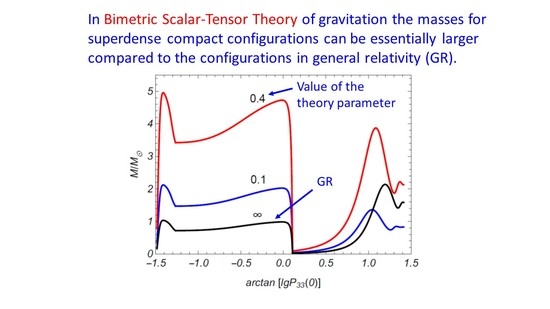
For a given value of the pressure at the center of the configuration, $P\left(0\right)$, the quantities $\nu \left(0\right)$, $\lambda \left(0\right)$, $\phi \left(0\right)$ and the mass M are determined by the matching conditions for the external and internal solutions on the surface of the gravitating body $r=r_1$, where $P\left(r_1\right)=0$. In Figure 1, we have plotted the dependence of the mass (in units of the solar mass $M_{\odot }$) of a superdense configuration as a function of the central pressure for separate values of the theory parameter $\zeta$ (numbers near the curves). In the numerical integration, we have used the equation of state from [30,31]. It is obtained from the relations (6.1) in [30] substituting the pressure and the chemical potential from the formulas (6.6), (6.7), (6.9) and (6.11) from that reference. The curves with $\zeta =\infty$ correspond to configurations in general relativity.

In general relativity, the configurations corresponding to the monotonically-increasing segment on the left of the first local maximum correspond to white dwarfs. The monotonically-increasing segment between the first and second local maxima corresponds to configurations that are unstable against radial perturbations. The monotonically-increasing segment between the second and third local maxima corresponds to neutron stars. Note that in BSTT, the issue of the stability of the static configurations requires an additional investigation. As seen from the graphs, depending on the value of the theory parameter $\zeta$, in BSTT, the masses of the corresponding configurations for a fixed value of the pressure at the center can be essentially larger compared to the corresponding values in general relativity. For large values of the parameter, $\zeta \gg 1$, the curves in BSTT and in general relativity are practically indistinguishable. Note that the study of neutron star masses presently has attracted considerable interest both in the fields of theory and observations (see, for instance, [32,33]). This, in particular, was motivated by the observation of neutron stars with masses near $2M_{\odot }$.

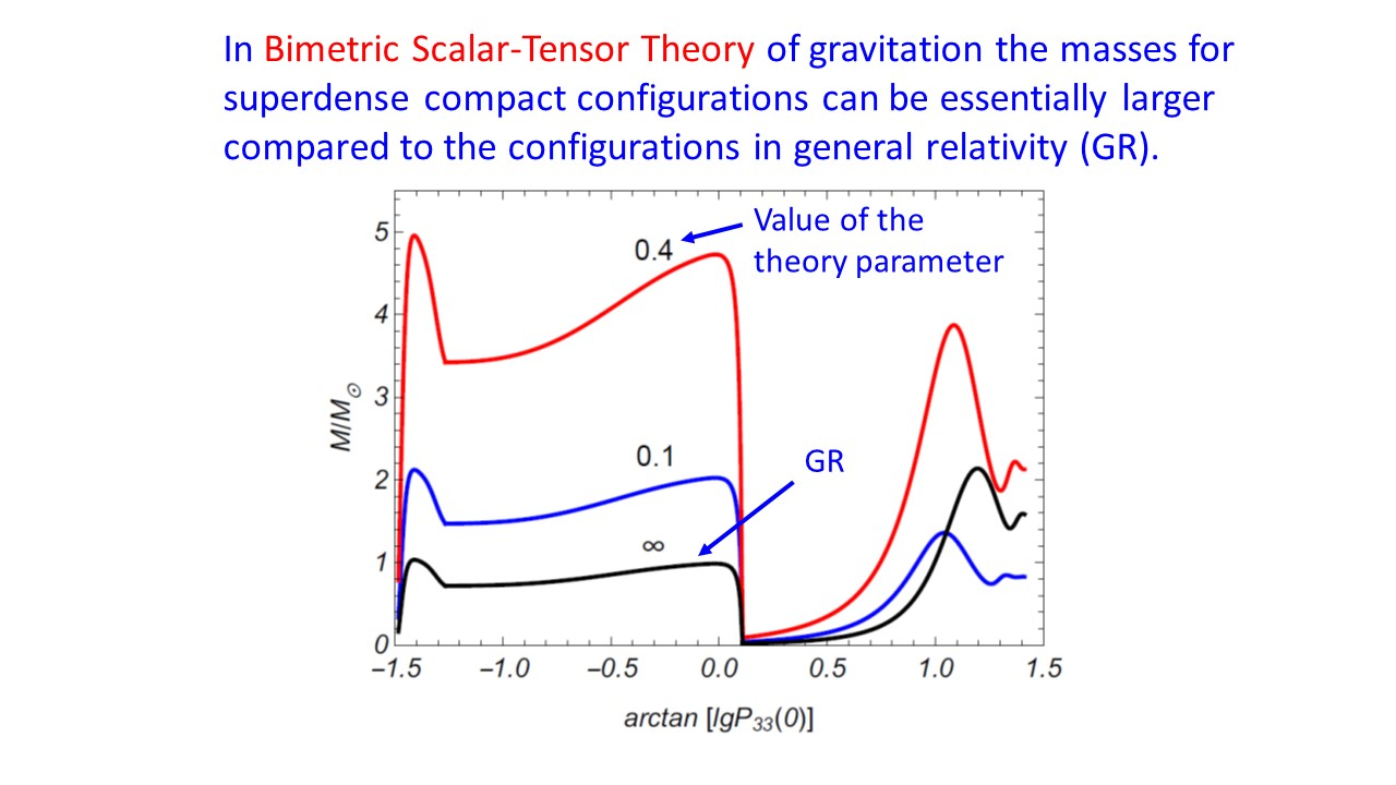
In addition to the mass of the configuration, the external geometry is determined by:

$$\beta =4\pi {\int }_0^{r_1}dr{r}^{2}P{e}^{3z-\nu }.$$

(19)

In terms of this parameter, one has $\alpha =3\beta /M$. In Figure 2, we have plotted the ratio $\beta /M_{\odot }$ as a function of the central pressure for the values of the theory parameter $\zeta =0.1,0.4,\infty$. As we could expect for configurations corresponding to white dwarfs, $\beta /M_{\odot }\ll 1$. Note that for the examples corresponding to Figure 2, one has $a>0$, and the external solution is given by the first formula in (13). The numerical analysis shows that the difference of that solution from the solution on general relativity with the same value of the mass is rather small. The numerical integration shows that for $\zeta >2$, the parameters of the configurations in BSTT are very close to those for general relativity.

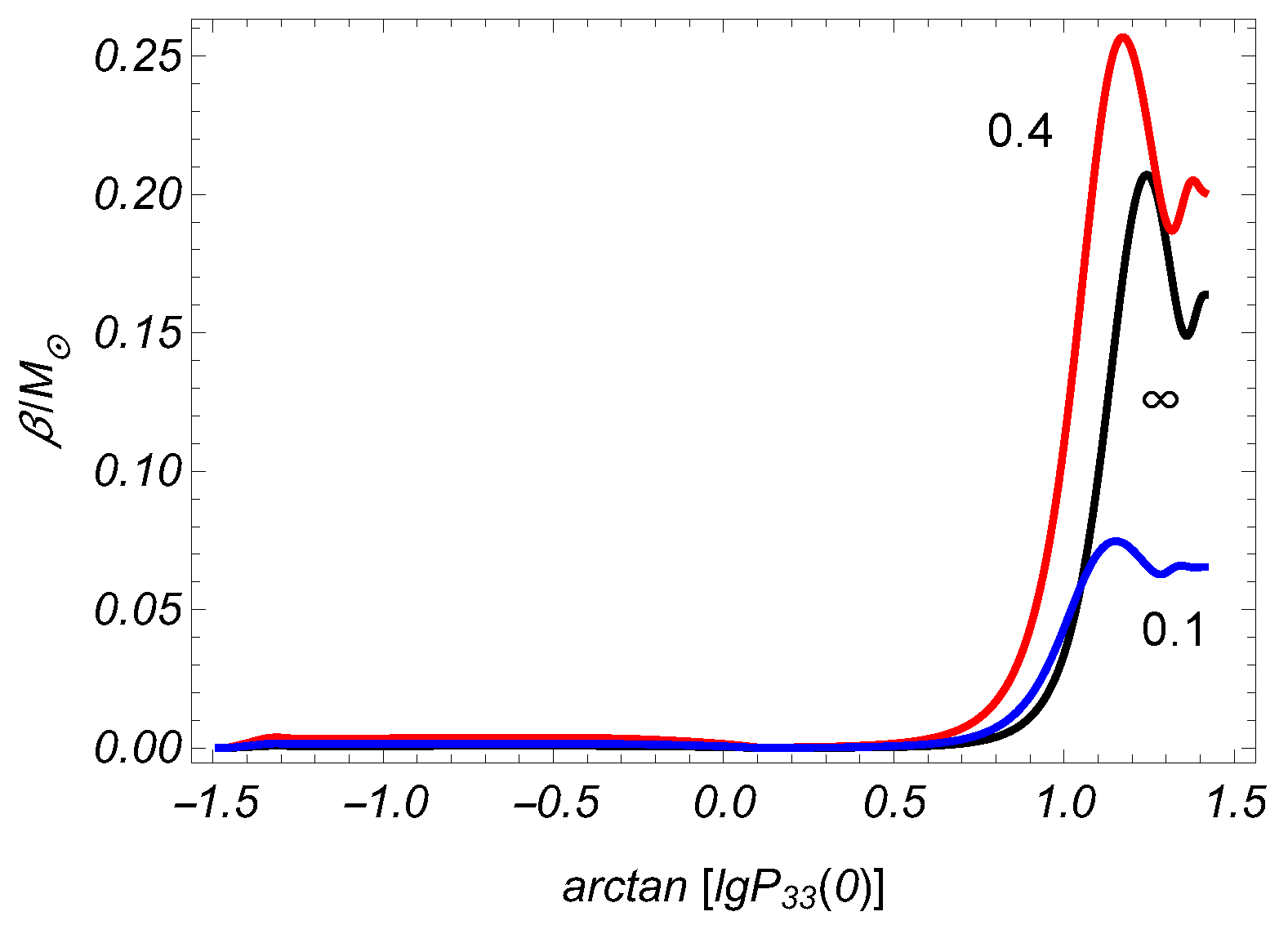
Figure 3 presents the radius of the configuration versus the central pressure for different values of the parameter $\zeta$ (numbers near the curves). The graphs show that, depending on the value of $\zeta$, the radii of the configurations may notably exceed the corresponding values in general relativity.

Let us consider examples of configurations in the variant of BSTT with $\zeta =0.4$, corresponding to a neutron star with the mass $M=1.5M_{\odot }$. For the equation of state we have used, one has $r_1\approx 36$ km and $\alpha \approx 0.044$. The numerical analysis shows that the difference of the corresponding external solution, given by the first formula in (13), from the solution of general relativity with the same value of the mass is rather small. In particular, the function $\phi \left(r\right)$ is a monotonically-increasing function outside the configuration and $1-\phi \left(r\right)/{\phi }_0<0.001$. This means that with the approach to the surface of the star in the exterior region, the effective gravitational constant increases. For this example, the external gravitational field is close to the one for a neutron star with the same mass in general relativity. The numerical integration inside the configuration shows that the function $\phi \left(r\right)$ monotonically increases in the interior region, as well, and the corresponding variation from the center to the surface is small, $\left[\phi \left(0\right)-\phi \left(r_1\right)\right]/{\phi }_0\approx 0.0012$. Hence, the effective gravitational constant takes its maximum value at the center of the configuration. The variations of the scalar field are relatively larger for larger values of the mass. For example, for the configuration with $M=3.8M_{\odot }$, one has $\phi \left(0\right)/{\phi }_0\approx 0.705$ and $\left[\phi \left(0\right)-\phi \left(r_1\right)\right]/{\phi }_0\approx 0.0087$. As in the previous case, the function $\phi \left(r\right)$ is monotonically increasing for all values of the radial coordinate. For this configuration, the value of the parameter $\alpha$ is larger, $\alpha \approx 0.135$, and in accordance with the analysis presented before, the variations of the scalar field are more significant.

5. Conclusions

In the present paper, we have investigated static spherically-symmetric configurations of gravitating masses in the simplest version of BSTT with a constant coupling function and with the zero cosmological function. The constraints on the coupling constant, obtained from the observations within the framework of the post-Newtonian approximation, are essentially weaker than those in usual scalar-tensor theories (Brans–Dicke theory). The corresponding external solution is given by (13) and (15). In addition to the mass, the solution depends on the parameter $\alpha$, which is determined in terms of the integral involving the pressure of the gravitating matter. For the integration of the field equations inside the configuration, we have used the equation of state from [30,31]. The corresponding numerical data are presented in Figure 1, Figure 2 and Figure 3. These results show that, for strong gravitational fields, depending on the value of the BSTT parameter $\zeta$, the characteristics of the superdense configurations may essentially differ from those in general relativity. Note that we have considered spherically-symmetric solutions with a variable gravitational scalar. The possibility for solutions with a constant scalar field has been discussed in [34,35].

References

- Clifton, T.; Ferreira, P.G.; Padilla, A.; Skordis, C. Modified gravity and cosmology. Phys. Rep. 2012, 513, 1–189. [Google Scholar] [CrossRef]
- Schmidt-May, A.; von Strauss, M. Recent developments in bimetric theory. J. Phys. A Math. Theor. 2016, 49, 183001. [Google Scholar] [CrossRef] [Green Version]
- Hinterbichler, K. Theoretical aspects of massive gravity. Rev. Mod. Phys. 2012, 84, 671. [Google Scholar] [CrossRef]
- De Rham, C.; Gabadadze, G. Generalization of the Fierz–Pauli action. Phys. Rev. D 2010, 82, 044020. [Google Scholar] [CrossRef]
- De Rham, C.; Gabadadze, G.; Tolley, A.J. Resummation of massive gravity. Phys. Rev. Lett. 2011, 106, 231101. [Google Scholar] [CrossRef] [PubMed]
- Hassan, S.F.; Rosen, R.A. Resolving the ghost problem in non-linear massive gravity. Phys. Rev. Lett. 2012, 108, 041101. [Google Scholar] [CrossRef] [PubMed]
- Hassan, S.; Rosen, R.A.; Schmidt-May, A. Ghost-free massive gravity with a general reference metric. J. High Energy Phys. 2012, 2012, 26. [Google Scholar] [CrossRef]
- Hassan, S.; Rosen, R.A. Confirmation of the secondary constraint and absence of ghost in massive gravity and bimetric gravity. J. High Energy Phys. 2012, 2012, 123. [Google Scholar] [CrossRef]
- Hassan, S.; Rosen, R.A. Bimetric gravity from ghost-free massive gravity. J. High Energy Phys. 2012, 2012, 126. [Google Scholar] [CrossRef]
- Volkov, M.S. Cosmological solutions with massive gravitons in the bigravity theory. J. High Energy Phys. 2012, 2012, 35. [Google Scholar] [CrossRef]
- Von Strauss, M.; Schmidt-May, A.; Enander, J.; Mörtsell, E.; Hassan, S. Cosmological solutions in bimetric gravity and their observational tests. JCAP 2012, 2012, 042. [Google Scholar] [CrossRef]
- Berg, M.; Buchberger, I.; Enander, J.; Mörtsell, E.; Sjörs, S. Growth histories in bimetric massive gravity. J. Cosmol. Astropart. Phys. 2012, 2012, 021. [Google Scholar] [CrossRef]
- Tamanini, N.; Saridakis, E.N.; Koivisto, T.S. The cosmology of interacting spin-2 fields. J. Cosmol. Astropart. Phys. 2014, 2014, 015. [Google Scholar] [CrossRef]
- Cai, Y.-F.; Easson, D.A.; Gao, C.; Saridakis, E.N. Charged black holes in nonlinear massive gravity. Phys. Rev. D 2013, 87, 064001. [Google Scholar] [CrossRef]
- Cai, Y.-F.; Duplessis, F.; Saridakis, E.N. F(R) nonlinear massive theories of gravity and their cosmological implications. Phys. Rev. D 2014, 90, 064051. [Google Scholar] [CrossRef]
- Cai, Y.-F.; Saridakis, E.N. Cosmology of F(R) nonlinear massive gravity. Phys. Rev. D 2014, 90, 063528. [Google Scholar] [CrossRef]
- Grigorian, L.S.; Saharian, A.A. Generalized bimetric theory of gravitation. Astrophysics 1990, 31, 359–368. [Google Scholar] [CrossRef]
- Grigorian, L.S.; Saharian, A.A. A new approach to the theory with variable gravitational constant. Astrophys. Space Sci. 1990, 167, 271–280. [Google Scholar] [CrossRef]
- Grigorian, L.S.; Saharian, A.A. Scalar-tensor bimetric theory of gravitation. I. Astrophys. 1990, 32, 491–500. [Google Scholar]
- Grigorian, L.S.; Saharian, A.A. New alternative for general relativity theory. Astrophys. Space Sci. 1991, 180, 39–45. [Google Scholar] [CrossRef]
- Will, C.M. Theory and Experiment in Gravitational Physics; Cambridge University Press: Cambridge, UK, 1993. [Google Scholar]
- Grigorian, L.S.; Saharian, A.A. Scalar-tensor bimetric theory of gravitation. II. Energy momentum tensor of the gravitational field. Astrophysics 1990, 33, 107–112. [Google Scholar]
- Grigorian, L.S.; Saharian, A.A. Integral conservation laws in BSTT. Astrophysics 1994, 37, 167–173. [Google Scholar] [CrossRef]
- Saharian, A.A. Radiation of gravitational waves in BSTT. Astrophysics 1993, 36, 423–430. [Google Scholar]
- Saharian, A.A. Modified EIH formalism in BSTT. Gravitational radiation. Astrophysics 1993, 36, 603–611. [Google Scholar] [CrossRef]
- Avakian, M.R.; Grigorian, L.S.; Saharian, A.A. Models of neutron stars in generalized scalar-tensor theory of gravitation. Astrophysics 1990, 35, 121–130. [Google Scholar]
- Babak, S.V.; Grishchuk, L.P. Energy-momentum tensor for the gravitational field. Phys. Rev. D 1999, 61, 024038. [Google Scholar] [CrossRef]
- Sahakian, G.S. Equilibrium Configurations of Degenerate Gaseous Masses; Halsted (Wiley): New York, NY, USA; Israel Program for Scientific Translations: Jerusalem, Israel, 1974. [Google Scholar]
- Avakian, M.R.; Grigorian, L.S.; Saharian, A.A. On Tolmen formula in scalar-tensor theories of gravitation. Astrophysics 1991, 34, 265–270. [Google Scholar]
- Grigorian, L.S.; Sahakian, G.S. Theory of superdense matter and degenerate stellar configurations. Astrophys. Space Sci. 1983, 95, 305–356. [Google Scholar] [CrossRef]
- Sahakian, G.S. Physics of Neutron Stars; JINR Publishing Department: Dubna, Russia, 1995. [Google Scholar]
- Özel, F.; Freire, P. Masses, radii, and the equation of state of neutron stars. Annu. Rev. Astron. Astrophys. 2016, 54, 401–440. [Google Scholar] [CrossRef]
- Horvath, J.E.; Valentim, R. The Masses of Neutron Stars. In Handbook of Supernovae; Alsabti, A., Murdin, P., Eds.; Springer: Cham, Switzerland, 2017. [Google Scholar]
- Saharian, A.A. Spherically-symmetric solutions of GR are partial solutions of BSTT. Astrophysics 1993, 36, 245–249. [Google Scholar]
- Kazarian, P.F.; Saharian, A.A. On Birkhoff’s theorem in BSTT. Astrophysics 1997, 40, 183–189. [Google Scholar] [CrossRef]
Figure 1.
The mass of a superdense star as a function of the central pressure . The numbers near the curves correspond to the values of the bimetric scalar-tensor theory (BSTT) parameter and . The curve corresponds to configurations in general relativity.
Figure 2.
The dependence of the ratio on the central pressure. The numbers near the curves correspond to the values of the BSTT parameter .
Figure 3.
The radius of a superdense star versus the central pressure. The numbers near the curves correspond to the values of the parameter . The curve corresponds to the results in general relativity.
© 2018 by the authors. Licensee MDPI, Basel, Switzerland. This article is an open access article distributed under the terms and conditions of the Creative Commons Attribution (CC BY) license (http://creativecommons.org/licenses/by/4.0/).
Share and Cite
MDPI and ACS Style
Grigorian, L.S.; Khachatryan, H.F.; Saharian, A.A. Models of Compact Stars in the Bimetric Scalar-Tensor Theory of Gravitation. Particles 2018, 1, 203-211. https://doi.org/10.3390/particles1010015
AMA Style
Grigorian LS, Khachatryan HF, Saharian AA. Models of Compact Stars in the Bimetric Scalar-Tensor Theory of Gravitation. Particles. 2018; 1(1):203-211. https://doi.org/10.3390/particles1010015
Chicago/Turabian StyleGrigorian, Levon Sh., Hrant F. Khachatryan, and Aram A. Saharian. 2018. "Models of Compact Stars in the Bimetric Scalar-Tensor Theory of Gravitation" Particles 1, no. 1: 203-211. https://doi.org/10.3390/particles1010015