
Reservoir Simulations of Hydrogen Generation from Natural Gas with CO2 EOR: A Case Study

1
Department of Hydrocarbon Reservoir and UGS Simulation, Oil and Gas Institute-National Research Institute, 25 A Lubicz Str., 31-503 Kraków, Poland
2
LOTOS Petrobaltic S.A.—ORLEN Group, 9 Stary Dwór Str., 80-758 Gdańsk, Poland
*
Author to whom correspondence should be addressed.
Energies 2024, 17(10), 2321; https://doi.org/10.3390/en17102321
Submission received: 11 April 2024
/
Revised: 25 April 2024
/
Accepted: 6 May 2024
/
Published: 11 May 2024
(This article belongs to the Section A5: Hydrogen Energy)
Abstract
:This paper addresses the problem of hydrogen generation from hydrocarbon gases using Steam Methane Reforming (SMR) with byproduct CO2 injected into and stored in a partially depleted oil reservoir. It focuses on the reservoir aspects of the problem using numerical simulation of the processes. To this aim, a numerical model of a real oil reservoir was constructed and calibrated based on its 30-year production history. An algorithm was developed to quantify the CO2 amount from the SMR process as well as from the produced fluids, and optionally, from external sources. Multiple simulation forecasts were performed for oil and gas production from the reservoir, hydrogen generation, and concomitant injection of the byproduct CO2 back to the same reservoir. EOR from miscible oil displacement was found to occur in the reservoir. Various scenarios of the forecasts confirmed the effectiveness of the adopted strategy for the same source of hydrocarbons and CO2 sink. Detailed simulation results are discussed, and both the advantages and drawbacks of the proposed approach for blue hydrogen generation are concluded. In particular, the question of reservoir fluid balance was emphasized, and its consequences were presented. The presented technology, using CO2 from hydrogen production and other sources to increase oil production, also has a significant impact on the protection of the natural environment via the elimination of CO2 emission to the atmosphere with concomitant production of H2.
1. Introduction
In Europe and around the world, hydrogen is gaining importance as a raw material, fuel, or energy carrier and storage medium due to the zero-emission transformation of energy systems [1]. Depending on the production methods, hydrogen can be green, blue, aqua, and white—called low-carbon hydrogen—and then grey, brown or black, yellow, turquoise, purple or pink, and red—although naming conventions can vary across countries and over time [2]. From an environmental protection perspective, the production of green and blue hydrogen—with effectively no or very low CO2 emission to the atmosphere—is the most desirable. At present, blue hydrogen, with an annual production of approximately 1 Mt, is mainly produced by reforming natural gas (Steam Methane Reforming—SMR), with an energy efficiency of 62% to 80% [3,4]. CO2 is a byproduct of the SMR process, and the resulting hydrogen is called grey hydrogen. This is how 62% of the world’s hydrogen is produced [1]. However, by injecting the obtained CO2 into underground geological structures for safe and permanent storage, the classification of the generated hydrogen is changed from grey to blue [5,6]. These structures include dedicated water-bearing formations as exemplified by the Quest plant in Canada [7]. Most of the operational and/or advanced preparation-stage blue hydrogen projects use depleted petroleum (mostly gas) reservoirs as CO2 storage structures. These include the Net-Zero Hydrogen Energy Complex project in Canada [8], Tabangao refinery project in Philippines [9], Changwon Industrial complex project in South Korea [10], and the Magnum project in the Netherlands [11]. The same type of CO2 sequestration structures are also considered in future blue hydrogen projects: the Acorn Aberdeenshire project [12], Net Zero Teesside project [13], Drax Humber cluster project [14], and H2H Saltend project [15] in the United Kingdom; the H-Vision project [16] and Blue Hydrogen plant project [17] in the Netherlands; the Preem project in Sweden [18]; and the HESC project in Australia [19].
An alternative way to utilize the CO2 as a byproduct resulting from the hydrogen generation process is to use it in the EOR method by injecting it into a partially depleted oil reservoir after the application of primary and secondary recovery methods [20,21]. This method provides a good alternative to CCS in aquifers [22,23]. The obtained CO2 can be used together with water in various EOR schemes such as CO2 WAG and CO2 SWAG [24,25,26]. The efficiency of these schemes can be further improved by selectively injecting these fluids [26,27]. Under typical reservoir conditions of pressure and temperature, injected CO2 becomes an oil-displacing fluid via the miscible displacement mechanism [28,29,30], causes a significant reduction in the final oil saturation and thus an increase in the final oil depletion factor [24]. However, in certain reservoirs, the high miscibility pressure presents a challenge for achieving miscibility under reservoir pressure conditions. Some additives, as shown in [31,32], effectively reduce the miscibility pressure by decreasing the interfacial tension (IFT) between oil and CO2, thus enhancing the miscible displacement of oil by CO2 [33]. In this study, it was found that the miscible displacement effect was achieved in the studied oil reservoir without the use of any additives mentioned earlier. However, the use of these additives and their impact on the oil recovery factor from the oil reservoir can be investigated in future studies. The method applied in our study for CO2 utilization is quite unique [34] and has not been used in the petroleum industry of Poland. Existing studies are restricted to the feasibility aspects of such projects and focus on the technological side of hydrogen generation and CO2 capture [35,36]. Moreover, they consider the cases of the hydrocarbon gas for the hydrogen generation originating from a gas reservoir different from an oil reservoir where the byproduct CO2 is injected.
In this paper, we present the analysis results concerning blue hydrogen generation combined with associated CO2 injection where the source of the hydrocarbon gas and the sink of the injected CO2 are the same oil reservoir. The analysis focused on reservoir aspects of the blue hydrogen generation and was performed by numerical modelling of the reservoir and simulations of the relevant processes. Following the construction and calibration of the reservoir model, multiple simulation forecasts were performed, taking into account the balancing of the produced hydrocarbon gas and the injected CO2 resulting from the SMR process and the separation of the produced gas. Performing various scenarios of the simulation forecasts allows the authors to assess the effectiveness of the adopted strategy and to draw conclusions concerning detailed conditions of the analysed process [24,35,37]. The authors used a compositional version of the commercial Eclipse reservoir simulator from Schlumberger, to generate simulation forecasts. This version allowed for accurate modeling of the reservoir fluid’s changing compositions during CO2 injection, as well as under varying pressure and temperature conditions. This resulted in the displacement of oil in a miscible manner. Then, the simulation results are discussed and both the advantages and drawbacks of the proposed blue hydrogen generation approach are concluded.
2. Static and Dynamic Models of the Reservoir
2.1. Static Model of the Reservoir
The B3 oil reservoir occurs in an anticlinal structural form, mapped within the sandstone of the Paradoxides paradoxissimus horizon of the Middle Cambrian in the area of the Łeba tectonic block. It is a layered structure. Crude oil saturates the sand series throughout the profile of the reservoir level located above an underlying aquifer.
From the top, the reservoir series is covered by tight geological strata of Upper Cambrian clay-carbonate formations, 3–6 m thick, overlaid by several-dozen-meter-high Ordovician clay-carbonate series, and then Silurian clay reservoirs, constituting a regional trap. Below the reservoir series, there are insulating clay-sandy sediments of the Eccaparadoxides oelandicus horizon. They are formed as mudstones and claystones with irregular interbeddings of loamy sandstones. They mark the boundary of the central part of the reservoir, where the oil–water contact has not been reached, while in the southern and northern parts, the level of oil–water contact is assumed as the lower boundary.
The model of the discussed structure is characterized by a 3D grid size of 46 × 155 × 17 blocks with an average horizontal dimension of a single 100 block and a vertical dimension not exceeding 4 m. The 3D view of this model is shown in Figure 1.
In the presented model, the average porosity ϕ = 7%, while the average horizontal permeability kh = 49 mD. The vertical to horizontal permeability anisotropy kv/kh = 0.25. Based on the geological model, a dynamic simulation model was built by supplementing it with typical relative permeability [38] and capillary pressure curves [39] and the reservoir fluid model presented below.
2.2. PVT Model of Hydrocarbon Formation Fluid
To determine the PVT model of the hydrocarbon reservoir fluid, the measured properties of the reservoir fluid from laboratory tests were used. For the multi-component reservoir simulation model, a fluid model was created using the PVTsim program [40] based on the SRK (Soave–Redlich–Kwong) state equation.
2.3. PVT Properties of Hydrocarbons
To determine the PVT properties of hydrocarbons for the reservoir simulation model, a bottom-hole sample from the producing well was used with the chemical composition given in Table 1.
Four types of PVT experiments were performed on the reservoir fluid sample with the above-mentioned chemical composition: bubble point pressure, constant mass study, differential vaporization, separation tests, and viscosity study. In the calibration procedure, the following parameters of the equation of state of individual fluid components were matched: critical pressure, critical temperature, acentricity coefficient, and five parameters of the LBC (Lohrenz–Bray–Clark) viscosity model. Based on the obtained model, tables of parameters required by the ECLIPSE 300 reservoir simulator were obtained.
2.4. PVT Properties of Formation Water
For formation water with density ρw = 1015 kg/m3 at temperature Tres = 62 °C and pressure P = 172 bar, the following properties were determined based on the standard correlations for reservoir brine:
- Water formation volume factor, Bw = 1.0092 m3/Nm3;
- Isothermal compressibility, cw = 5 10−4 1/bar;
- Viscosity, μw = 0.47 cP;
- Coefficient of viscosity change with pressure, .
2.5. History Matching
As a result of oil production without the use of any EOR from the reservoir conducted since 1992, the average reservoir pressure dropped by approx. 16% according to initial pressure up to the present. On average, 11 producers worked in the field, some of which were reconstructed.
As a result of the modifications of the reservoir fluid model along with the modification of the endpoints for the relative water permeability curve, a correct fit of the simulation model results for the bottom-hole pressure, gas/oil ratio, and water cut to the observed points was obtained. These adjustments for an exemplary production well are shown in Figure 2, Figure 3 and Figure 4. The mean and standard deviation of the measured GOR were calculated, and the results of the simulation were found to be within the standard deviation range of the mean value, as presented in Figure 3. The error bars are not visible in Figure 2 and Figure 4 for WCT and BHP/Pini, respectively, due to their high accuracy (error below 1%).
The average reservoir pressure throughout the entire history of the oil production from the reservoir did not fall below the saturation pressure, as a result of which the gas/oil ratio obtained from the simulation model for production wells remained at a constant level of the initial gas/oil ratio.
As a result of injecting water into the reservoir, its amount in the reservoir increased as well as water saturation and mobility. In addition, the dominant direction of water migration is the direction from the injectors to the producers along the induced pressure gradients. As a result, oil production decreased relatively quickly.
3. Simulation Forecasts of the EOR Process with CO2 Injection
3.1. General Assumptions
To assess the effectiveness of the adopted EOR strategy, prognostic scenarios were developed covering the development strategies for the enhanced oil production from the reservoir from 1 June 2022 to 1 June 2042. Other basic assumptions for oil production from the reservoir are the following (see the Nomenclature section for the detailed definitions of used quantities):
- –
- Initial oil production rate: qo,prod,0 = 600 Nm3/d;
- –
- Composition of the injected gas: cCO2inj = 100%;
- –
- Water injection rate in terms reservoir volume: qvw,inj = qv,prod − qvCO2,inj [Rm3/d];
- –
- Minimum water injection rate: qw,inj,min = qw,prod [Sm3/d];
- –
- List of producers: P1, P2, P3, P4, P5, P6, P7, P8, P9, P10, P11;
- –
- List of water/CO2 injectors: I1, I2, I3, I4, I5, and converted wells;
- –
- Rate of hydrocarbon gas used for the rig’s consumption: qg,cons = 18,000 Nm3/d;
- –
- Maximum rate of injected CO2 originating from the SMR process of the hydrocarbons in the produced gas and separated from that gas, assuming 100% efficiency of these processes;
- –
- Maximum rate of injected CO2 originating from the outside sources (determined by the capacity of the tanker and the cyclical nature of deliveries): qCO2ext = 500,000 Nm3/d;
- –
- Minimum bottom-hole pressure of producers, Pbhp,prod,min = 90 bar;
- –
- Maximum bottom-hole pressure of CO2 injectors, Pbhp,injCO2,max = 220 bar;
- –
- Maximum bottom-hole pressure of water injectors, Pbhp,injH2O,max = 250 bar;
- –
- Contributions of individual producing wells to the total produced stream according to the last year’s historical data;
- –
- Contributions of individual injecting wells to the total injected stream according to the well injection potentials.
3.2. SMR
In order to calculate the volume of the CO2 stream obtained from the SMR [3,41] and the other component from the separation process on the produced gas, the algorithm shown in Figure 5 was incorporated into the simulation model. This implementation was made possible through the Eclipse simulator’s specific capabilities, (by so-called user-defined quantities). This capability enables the implementation of external algorithms, such as an injection control algorithm, based on the production of CO2.
In the algorithm presented above, the gas balance (hydrocarbons and CO2) was used in the production of hydrogen in the SMR reaction from hydrocarbon gas produced in the process of oil production from the reservoir coupled with CO2 reinjection.
The effective formula of hydrogen generation in the SMR reaction for the hydrocarbon component of a carbon number n is given by the following:
i.e., each mole of such component produces n moles of CO2, which determines the basic calculation of the analyzed process. In particular, the rate of CO2 available for the injection, qCO2,inj, into a target reservoir is a function of the known gas rates and their compositions, and it is calculated according to the following formula:
where uCO2,inj is the CO2 molar injection rate that takes into account the CO2 separated from the reservoir production fluids and combined with the CO2 from the SMR, uCO2,prod:
where uCO2,SMR is the molar rate of CO2 from the SMR process:
CnH2m + 2nH2O → (2n + m)H2 + nCO2
qCO2,inj = uCO2,inj MWCO2/ρCO2
uCO2,inj = uCO2,SMR + uCO2,prod
Here, uCH,SMR is the molar rate of the hydrocarbon components in the SMR inflow gas given by the following:
where the molar rate of the reservoir gas production, ug,prod, is reduced by the gas consumed by the production/injection system, ug,cons, and by the CO2 separated from the produced gas, uCO2,prod.
uCH,SMR = ug,prod − ug,cons − uCO2,prod
These molar rates result from their volume rates: qg,prod, qg,cons, qCO2,prod, respectively:
ug,prod = qg,prod ρg,prod/MWg,prod
ug,cons = qg,cons ρg,prod/MWg,prod
uCO2,prod = qCO2,prod ρCO2/MWCO2
Here, the mole weight of the produced gas is given by the following:
The other quantities of the above formulae are defined in the Nomenclature section.
3.3. Base Forecast—Scenario I
Scenario I assumes the continuation of oil production with constant water injection. Its results, shown in Figure 6, are determined by the limitation of the minimum bottom-hole pressure in producers, Pbhp, prod, min.
To maintain oil production at a high level throughout the forecast period, it was necessary to maintain the average reservoir pressure at a constant level, which was achieved by balancing the produced fluids by injecting water into the reservoir (Figure 6 and Figure 7).
For this purpose, water injectors located at the water–oil contour in the eastern part of the field were used. As a result of field operation at a constant average reservoir pressure (above saturation pressure), a decrease in the gas production rate was obtained as a consequence of a decrease in the oil production rate (Figure 8).
The effect of intensive water injection into the reservoir is the reduction in oil saturation to the critical value of Socr = 0.30 (Figure 9).
3.4. Forecasts with the Injection of CO2 from the SMR—Scenario II
Using the gas flow diagram for the production of H2 and CO2 and the separation of CO2 from the produced gas (Figure 5), four prognostic Scenarios were prepared, assuming the injection of CO2 into the reservoir through selected wells, according to Table 2.
In these scenarios, a very small improvement in oil production was obtained (Figure 12), which was related to the relatively small amount of CO2 from the hydrocarbon gas SMR and the separation of the produced gas.
Moreover, three years after the forecast started, gas consumption by the production platform exceeded its production, meaning that the production of hydrogen and CO2 ended. This is related to the decrease in the oil production rate and, consequently, the decline in the hydrocarbon gas production rate (Figure 13).
As in Scenario I, water is injected into the reservoir, which, together with the injected gas, balances the produced fluids (Figure 14).
As a result of the end of the H2 and CO2 production stage in 2026, only water is injected into the reservoir. Due to the relatively small volume of injected CO2, the resulting miscible displacement effect is local (Figure 15) and does not have a significant impact on the oil production from the reservoir.
3.5. Forecasts with the Injection of Additional CO2—Scenario III
Since the forecasts for Scenarios of group II showed limited miscible displacement of a local nature caused by a relatively low rate of the injected CO2, we conducted additional Scenarios with an increased rate of injection of CO2 from the deliveries of a tanker with a capacity of ~30,000 m3 tonnes of CO2, which delivers to the rig platform every month, as a result increasing the volume of CO2 injected by an additional 500,000 Nm3/d. Table 3 lists four Scenarios that differ in the CO2 injecting wells.
As a result of increasing the injection of CO2 into the reservoir, an increase in oil production was obtained for all Scenarios III in the range of 36 to 91% compared to Scenario I. The largest increase was obtained in Scenario IIIc, for which CO2 was injected by I2, I3, I4, and I6 (converted from P1) wells while wells I1 and I5 were used to reinject the produced water. It should be noted that for the considered Scenario III variations, an increase in the average reservoir pressure (Figure 16) above the original value is observed, although the dynamic pressure at the bottom of the injecting wells did not exceed the maximum assumed value.
As a result of the intensive injection of CO2 into the reservoir, its breakthrough into the producers was observed as an increase in the production of CO2-contaminated gas, which in turn translates into an increase in the injection of CO2 into the reservoir (Figure 17).
Intensive injection of CO2 and increased reservoir pressure expands the region covered by miscible displacement, which results in a drop in critical oil saturation to Sgcr = 0 (Figure 18 and Figure 19).
The basic results of the nine Scenarios of the field production in the forecast period from 2022 to 2042 are presented in Table 4. They include the volume of total production and injection of water and gas as well as the total oil production in the forecast period, along with the relative increase in oil production in relation to Scenario I (base) and the replacement factor corresponding to the volume/mass of injected CO2 needed to increase oil production by 1 Nm3/1 kg. These results mean that a significant amount of CO2 must be injected to increase oil production (scenarios III vs. II). At the same time, a significant increase in the volume of injected CO2 (scenario III) leads to a significant increase in oil production, reaching over 90% in relation to the Scenario with the injection of water only (option I). The measurement of the effectiveness of the method of displacing oil with the injected CO2 as part of the miscible displacement mechanism is the so-called replacement factor, specifying the amount (volume/mass) of injected CO2 needed to displace a unit amount (1 Nm3/1 kg) of oil. This coefficient varies widely from 4 to 20 kg of CO2 per 1 kg of crude oil. This result means a strong dependence on the effectiveness of the method used in the selection of the system of injecting wells [42], which differed in the individual Scenario III variations. This means that there exists a potential opportunity to optimize the analyzed method by selecting the number and location of the injecting and producing wells.
4. Summary and Conclusions
This paper presents the analysis of a hydrogen generation SMR process from the hydrocarbon gas produced from an oil reservoir. The hydrogen is made blue by the injection of the CO2 resulting from SMR back into the same reservoir and using the gas as an oil-displacing fluid within the EOR method. The analysis was performed as a case study for a realistic oil reservoir located in the Baltic Shelf of Poland using a numerical reservoir modelling and simulation approach. To this aim, a compositional reservoir model was constructed and calibrated based on the 30-year production history of the reservoir. For the analysis, an algorithm was built and implemented in the model to calculate the amount of CO2 originating from the SMR process, the separation process of the produced fluids, and, optionally, CO2 delivered from external sources. To assess the impact of the v injection as an EOR method on increasing the oil depletion factor, multi-scenario simulation forecasts were made, differing in the volume of CO2 injected and the number and localisation of wells involved for CO2 and associated water injection. Quantitative results for 9 scenarios in the form of reservoir fluids productions including the changes in oil production and replacement factors are presented and discussed. These results were supplemented with a detailed analysis of oil saturation distributions for the selected, significant scenarios.
The main conclusion from the performed analysis indicates the proposed approach’s general effectiveness in generating blue hydrogen with concomitant, in-place usage of associated CO2 in the EOR method. Compared with other studies of blue hydrogen generation where the source of produced hydrocarbon gas and the sink of injected CO2 were different reservoirs, this study addresses the case of the hydrocarbon gas originating from the same reservoir that the byproduct CO2 is injected into. The advantage of the analyzed case is that there is no need for long-distance transportation of both the hydrocarbon gas from the production manifold to the SMR installation and the CO2 from the SMR output to the injection manifold. The additional gain in the approach comes from the EOR process and requires more detailed discussion. Under appropriate conditions of reservoir temperature and pressure and in reservoir regions covered by the injected CO2, partial or complete miscible oil displacement occurs, resulting in a reduction in the final oil saturation below the initial residual saturation, thus increasing the ultimate oil recovery factor. While the temperature and pressure conditions for the miscible displacement are typically met—as in the studied case—the extension of the reservoir volume covered by the injected CO2 is limited due to the restricted amount of CO2 from the SMR process. In principle, from the stoichiometry of the SMR, it follows that the volume of the CO2 is only a fraction of the produced oil volume. In particular, the CO2 production coefficient defined as the reservoir volume of injected CO2 obtained from one reservoir cubic meter of produced oil amounts to about 55% under the reservoir conditions of the studied case. Moreover, additional reduction in available CO2 may result from such factors as consumption of the produced hydrocarbon gas by production/injection system. In the analyzed case, this factor reduces the CO2 production coefficient down to 13%. Another factor of this type is the efficiency of v capturing from the SMR process, which can range between 50% and 99%, depending on the adopted technology. An additional factor that may influence the CO2 production coefficient is the process of oil degasification in the reservoir and the formation of a secondary gas cap due to a decrease in reservoir pressure when the reservoir fluid production is not balanced by fluid injection. To avoid such difficulties and enhance the EOR effectiveness, it is advisable to supplement the v from the SMR process with CO2 from additional external sources as performed in the studied case. Another way to compensate for the fluid imbalance may be realized by the additional injection of a fluid other than CO2. In the analyzed case, water injection was applied for this purpose. It should be noted that sooner or later breakthrough of the injected CO2 into production wells is unavoidable, thus leading to the necessity of a special installation to be used to separate CO2 from hydrocarbon components in the produced gas and the separated CO2 to be reinjected into the reservoir. It is important to consider that both the installation of SMR and the installation for separating CO2 from the extracted gas require extra space on the production platform. However, since the usable area of these platforms is already highly utilized, this could result in high investment costs. The final stage of the proposed approach to blue hydrogen generation may include the injection of additional CO2 to take advantage of the full reservoir sequestration volume.
Author Contributions
Conceptualization, K.M., W.S. and J.T.; methodology, W.S. and K.M.; software, K.M.; validation, W.S. and K.M.; formal analysis, W.S. and K.M.; investigation, W.S. and K.M.; resources, K.M., W.S., J.T. and A.L.; data curation, K.M., J.T. and A.L.; writing—original draft preparation, K.M. and W.S.; writing—review and editing, W.S. and K.M. All authors have read and agreed to the published version of the manuscript.
Funding
This research was carried out as part of the project: “Optimization of the operation of an oil field using carbon dioxide from the production of blue hydrogen” in Polish: “Optymalizacja pracy złoża ropy naftowej z wykorzystaniem dwutlenku węgla pochodzącego z produkcji niebieskiego wodoru”, which is funded by the Polish Ministry of Education and Science, Grant No. DK-4100-1/22. The authors would like to express their gratitude to the Polish Ministry of Education and Science for funding this research.
Data Availability Statement
Data available on request due to restrictions.
Conflicts of Interest
The authors declare no conflicts of interest.
Nomenclature
| Latin: | |
| BHP | bottom hole pressure [bar], |
| Bw | water formation volume factor [Rm3/Sm3], |
| cCO2,inj | mole fraction of CO2 in the injected gas [-], |
| cw | isothermal compressibility of water [1/bar], |
| DGinj | total CO2 injection [Sm3], |
| DNp | increase in total oil production [Sm3], |
| GOR | gas-oil ratio [-], |
| Gp | total gas production [Sm3], |
| kh | horizontal permeability [mD], |
| kv | vertical permeability [mD], |
| MWCO2 | molar weight of CO2 [kg/kmol], |
| MWi | molar weight of the i-th component in the produced gas [kg/kmol], |
| MWg,prod | molar weight of produced gas [kg/kmol], |
| Np | total oil production [Sm3], |
| Pini | initial reservoir pressure [bar], |
| Pbhp,prod,min | minimum bottom-hole pressure of producers [bar], |
| Pbhp,inj,CO2,max | maximum bottom-hole pressure of CO2 injectors [bar], |
| Pbhp,inj,H20,max | maximum bottom-hole pressure of water injectors [bar], |
| qCO2,inj | CO2 injection rate [Sm3/d], |
| qCO2,ext | the maximum rate of injected CO2 originating from the outside sources [Sm3/d], |
| qv,CO2,inj | CO2 injection rate in terms of reservoir volume [Rm3/d], |
| qg,prod | gas production rate [Sm3/d], |
| qg,cons | gas consumption rate [Sm3/d], |
| qo,prod | oil production rate [Sm3/d], |
| qw,prod | water production rate [Sm3/d], |
| qw,inj | water injection rate [Sm3/d], |
| qv,w,inj | water injection rate in terms of reservoir volume [Rm3/d], |
| qw,inj,min | minimum water injection rate [Sm3/d], |
| qv,prod | fluids production rate in terms of reservoir volume [Rm3/d], |
| Socr | critical oil saturation [-], |
| ug,prod | gas production molar rate [kmol/d], |
| ug,cons | gas consumption molar rate [kmol/d], |
| uCO2,prod | CO2 production molar rate [kmol/d], |
| uCH,SMR | SMR inflow molar rate [kmol/d], |
| uCO2,SMR | SMR outflow CO2 molar rate [kmol/d], |
| uCO2,inj | CO2 injection molar rate [kmol/d], |
| WCT | water cut [-], |
| Wp | total water production [Sm3], |
| Winj | total water injection [Sm3]. |
| Greek: | |
| coefficient of viscosity change with pressure [1/bar], | |
| ρCH,prod | density of produced gas hydrocarbon components [kg/Sm3], |
| ρg,prod | produced gas density [kg/Sm3], |
| ρw | water density [kg/Sm3], |
| φ | porosity [%]. |
| Subscripts: | |
| 0 | value at the beginning of the forecast. |
References
- IEA. Global Hydrogen Review 2022. 2022. Available online: https://www.iea.org/reports/global-hydrogen-review-2022 (accessed on 5 September 2023).
- Arcos, J.M.M.; Santos, D.M.F. The Hydrogen Color Spectrum: Techno-Economic Analysis of the Available Technologies for Hydrogen Production. Gases 2023, 3, 25–46. [Google Scholar] [CrossRef]
- Simpson, A.P.; Lutz, A.E. Exergy analysis of hydrogen production via steam methane reforming. Int. J. Hydrog. Energy 2007, 32, 4811–4820. [Google Scholar] [CrossRef]
- Baykara, S.Z. Hydrogen: A brief overview of its sources, production and environmental impact. Int. J. Hydrog. Energy 2018, 43, 10605–10614. [Google Scholar] [CrossRef]
- Katebah, M.; Linke, P. Analysis of hydrogen production costs in Steam-Methane Reforming considering integration with electrolysis and CO2 capture. Clean. Eng. Technol. 2022, 10, 100552. [Google Scholar] [CrossRef]
- Shahid, M.Z.; Kim, J.-K. Design and economic evaluation of a novel amine-based CO2 capture process for SMR-based hydrogen production plants. J. Clean. Prod. 2023, 402, 136704. [Google Scholar] [CrossRef]
- Rock, L.; O’Brien, S.; Tessarolo, S.; Duer, J.; Bacci, V.O.; Hirst, B.; Randell, D.; Helmy, M.; Blackmore, J.; Duong, C.; et al. The Quest CCS Project: 1st Year Review Post Start of Injection. Energy Procedia 2017, 114, 5320–5328. [Google Scholar] [CrossRef]
- Air Products Announces Multi-Billion Dollar Net-Zero Hydrogen Energy Complex in Edmonton, Alberta, Canada, 6 June 2021. Available online: https://hydrogen-central.com/air-products-multi-billion-dollar-net-zero-hydrogen-energy-complex-edmonton-alberta-canada/ (accessed on 8 September 2023).
- First Integrated Hydrogen Manufacturing Facility in the Philippines. 2020. Available online: https://pilipinas.shell.com.ph/sustainability/pilipinas-shell-annual-sustainability-report-2019/first-integrated-hydrogen-manufacturing-facility.html (accessed on 8 September 2023).
- Production of Blue Hydrogen Begins in Changwon City. 2021. Available online: https://energynews.biz/production-of-blue-hydrogen-begins-in-changwon-city/ (accessed on 8 September 2023).
- Equinor, Evaluating Conversion of Natural Gas to Hydrogen, 7 July 2017. Available online: https://www.equinor.com/news/archive/evaluating-conversion-natural-gas-hydrogen (accessed on 8 September 2023).
- Acorn, Projects CCS. Available online: https://www.theacornproject.uk/projects (accessed on 8 September 2023).
- Net Zero Teesside. Available online: https://www.netzeroteesside.co.uk/ (accessed on 8 September 2023).
- Drax, Leading Energy Companies Announce New Zero-Carbon UK Partnership. 2019. Available online: https://www.drax.com/press_release/energy-companies-announce-new-zero-carbon-uk-partnership-ccus-hydrogen-beccs-humber-equinor-national-grid/ (accessed on 8 September 2023).
- Equinor, H2H Saltend. Available online: https://www.equinor.com/energy/h2h-saltend (accessed on 8 September 2023).
- H-vision. H-vision Is Ready for the Next Phase. Available online: https://www.h-vision.nl/en (accessed on 9 August 2023).
- Den Helder. Blue Hydrogen Factory in Den Helder in Sight. Available online: https://portofdenhelder.nl/news/blue-hydrogen-factory-in-den-helder-in-sight (accessed on 8 September 2023).
- Aker Solutions. Aker Solutions Starts CCS Test Program at Preem Refinery in Sweden. 26 May 2020. Available online: https://www.akersolutions.com/news/news-archive/2020/aker-solutions-starts-ccs-test-program-at-preem-refinery-in-sweden/ (accessed on 8 September 2023).
- HESC. Hydrogen Gas Now Produced at Latrobe Valley Site. 2 February 2021. Available online: https://www.hydrogenenergysupplychain.com/hesc-project-milestone-hydrogen-gas-now-produced-at-latrobe-valley-site/ (accessed on 8 September 2023).
- Hill, L.B.; Li, X.; Wei, N. CO2-EOR in China: A comparative review. Int. J. Greenh. Gas Control 2020, 103, 103173. [Google Scholar] [CrossRef]
- Szott, W.; Łętkowski, P.; Gołąbek, A.; Miłek, K. Ocena efektów wspomaganego wydobycia ropy naftowej i gazu ziemnego z wybranych złóż krajowych z zastosowaniem zatłaczania CO2 (Assessment of EOR/EGR processes by CO2 injection for selected Polish oil and gas reservoirs). Pr. Nauk. INiG Nr 2012, 184, 35. [Google Scholar]
- Wang, F.; Liao, G.; Su, C.; Wang, F.; Ma, J.; Yang, Y. Carbon emission reduction accounting method for a CCUS-EOR project. Pet. Explor. Dev. 2023, 50, 989–1000. [Google Scholar] [CrossRef]
- Lindeberg, E.; Grimstad, A.-A.; Bergmo, P.; Wessel-Berg, D.; Torsæter, M.; Holt, T. Large Scale Tertiary CO2 EOR in Mature Water Flooded Norwegian Oil Fields. Energy Procedia 2017, 114, 7096–7106. [Google Scholar] [CrossRef]
- Miłek, K.; Szott, W. Zastosowanie symulacji złożowych do analizy porównawczej procesu EOR na przykładzie wybranych metod wspomagania (Application of reservoir simulations for comparative analysis of EOR by selected methods). Nafta-Gaz 2015, 3, 167–176. [Google Scholar]
- Karimaie, H.; Bamshad Nazarian, B.; Terje Aurdal, T.; Nøkleby, P.H.; Hansen, O. Simulation Study of CO2 EOR and Storage Potential in a North Sea Reservoir. Energy Procedia 2017, 114, 7018–7032. [Google Scholar] [CrossRef]
- Szott, W.; Miłek, K. Analysis of the enhanced oil recovery process through a bilateral well using WAG-CO2 based on reservoir simulation. Part I—Synthetic reservoir model. Nafta-Gaz 2018, 4, 270–278. [Google Scholar] [CrossRef]
- Szott, W.; Miłek, K. Analysis of the enhanced oil recovery process through a bilateral well using WAG-CO2 based on reservoir simulation. Part II—Real reservoir model. Nafta-Gaz 2018, 7, 62–69. [Google Scholar] [CrossRef]
- Benham, A.L.; Dowden, W.E.; Kunzman, W.J. Miscible Fluid Displacement—Prediction of Miscibility. Trans. AIME 1960, 219, 229–237. [Google Scholar] [CrossRef]
- Shen, B.; Yang, S.; Gao, X.; Li, S.; Yang, K.; Hu, J.; Chen, H. Interpretable knowledge-guided framework for modelling minimum miscible pressure of CO2-oil system in CO2-EOR projects. Eng. Appl. Artif. Intell. 2023, 118, 105687. [Google Scholar] [CrossRef]
- Habera, Ł. Aspekty termodynamiczne zatłaczania dwutlenku węgla w procesach intensyfikacji wydobycia ropy naftowej i gazu ziemnego (EOR/EGR) (Thermodynamic aspects of carbon dioxide injection in enhanced oil/gas recovery processes (EOR/EGR). Pr. Nauk. Inst. Naft. Gazu 2016. [Google Scholar] [CrossRef]
- Ahmadi, Y. Relationship between Asphaltene Adsorption on the Surface of Nanoparticles and Asphaltene Precipitation Inhibition During Real Crude Oil Natural Depletion Tests. Iran. J. Oil Gas Sci. Technol. 2021, 10, 69–82. Available online: http://ijogst.put.ac.ir (accessed on 1 April 2024).
- Ahmadi, Y.; Mansouri, M.; Jafarbeigi, E. Improving Simultaneous Water Alternative Associate Gas Tests in the Presence of Newly Synthesized γ-Al2O3/ZnO/Urea Nano-Composites: An Experimental Core Flooding Tests. ACS Omega 2023, 8, 1443–1452. [Google Scholar] [CrossRef]
- Li, S.; Zhu, J.; Wang, Z.; Li, M.; Wei, Y.; Zhang, K. Chemical strategies for enhancing CO2-Hydrocarbon miscibility. Sep. Purif. Technol. 2024, 337, 126436. [Google Scholar] [CrossRef]
- Penspen, Miller DF1, CCS Project. Available online: https://www.penspen.com/experience/miller-df1-ccs-project/ (accessed on 8 September 2023).
- Terrien, P.; Lockwood, F.; Granados, L.; Morel, T. CO2 Capture from H2 Plants: Implementation for EOR. Energy Procedia 2014, 63, 7861–7866. [Google Scholar] [CrossRef]
- IEAGHG. Techno-Economic Evaluation of SMR Based Standalone (Merchant) Plant with CCS, 2017/02. Available online: https://ieaghg.org/exco_docs/2017-02.pdf (accessed on 1 April 2024).
- Jarrell, P.; Fox, C.; Stein, M.; Webb, S. Practical Aspects of CO2 Flooding. SPE Monogr. 2002, 22, 1–10. [Google Scholar]
- Corey, A.T. The interrelation between gas and oil relative permeabilities. Prod. Mon. 1954, 19, 38–41. [Google Scholar]
- Brooks, R.H.; Corey, A.T. Hydraulic Properties of Porous Media; Hydrological Paper 3; Colorado State University: Fort Collins, CO, USA, 1964; pp. 22–27. [Google Scholar]
- Manual PVTSim. Available online: https://www.scribd.com/document/289452761/PVTSim-Manual# (accessed on 8 September 2023).
- García, L. Hydrogen production by steam reforming of natural gas and other nonrenewable feedstocks. In Compendium of Hydrogen Energy, Hydrogen Production and Purification; A volume in Woodhead Publishing Series in Energy; Woodhead Publishing: Cambridge, UK, 2015. [Google Scholar]
- Luboń, K. Influence of Injection Well Location on CO2 Geological Storage Efficiency. Energies 2021, 14, 8604. [Google Scholar] [CrossRef]
Figure 1.
Three-dimensional view of the model.

Figure 2.
The result of the bottom pressure matching process for an example well.

Figure 3.
The result of the gas–oil ratio matching process for an example well.
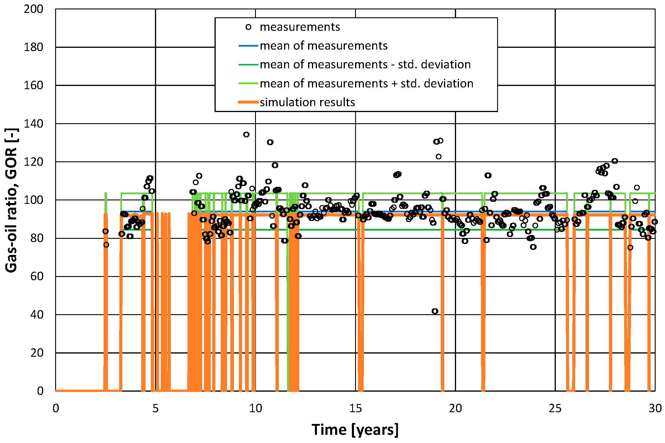
Figure 4.
The result of the water cut matching process for an example well.

Figure 5.
Diagram of gas flow in the project.

Figure 6.
Scenario I. Reservoir pressure, oil rate, and total oil production.

Figure 7.
Scenario I. Rate and total water production and injection.
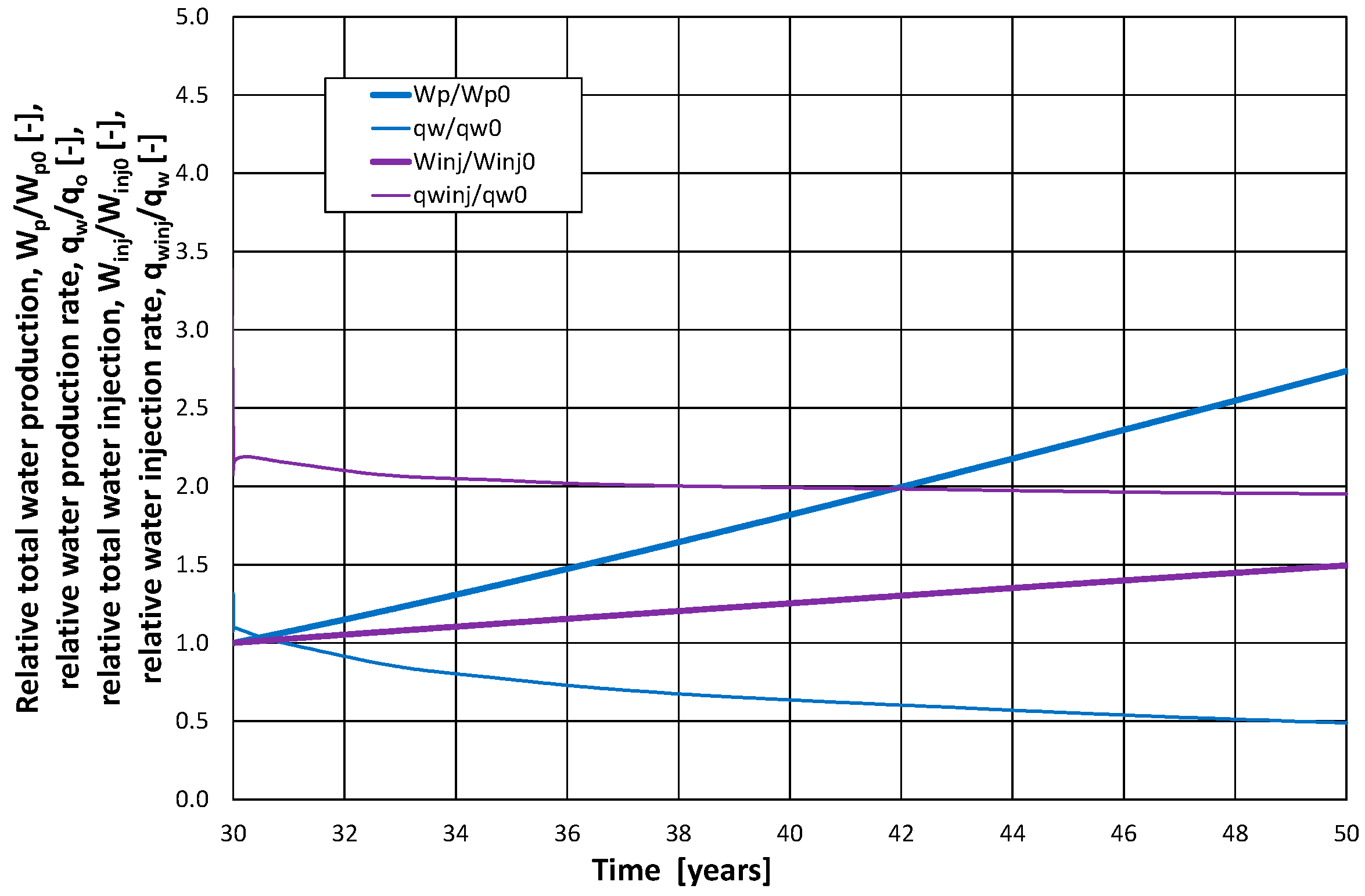
Figure 8.
Rate and total gas production.

Figure 9.
Scenario I. Distribution of oil saturation on a vertical cross-section along the main axis of the structure passing through the P1 well at the end of the forecast in 2042.
Figure 9.
Scenario I. Distribution of oil saturation on a vertical cross-section along the main axis of the structure passing through the P1 well at the end of the forecast in 2042.

Figure 10.
Distribution of oil saturation in the top layers of the reservoir at the beginning of the forecast in 2023.
Figure 10.
Distribution of oil saturation in the top layers of the reservoir at the beginning of the forecast in 2023.

Figure 11.
Scenario I. Distribution of oil saturation in the top layers of the reservoir at the end of the forecast in 2042.
Figure 11.
Scenario I. Distribution of oil saturation in the top layers of the reservoir at the end of the forecast in 2042.

Figure 12.
Scenario IIa, IIb, IIc, IId. Reservoir pressure and total oil production.

Figure 13.
Scenarios IIa, IIb, IIc, IId. Rate of gas production and CO2 injection.

Figure 14.
Scenarios IIa, IIb, IIc, IId. Rate of production and injection of water.

Figure 15.
Scenario IIb. Distribution of oil saturation at the vertical cross-section along the main axis of the structure passing through the I6 well at the end of the forecast in 2042.
Figure 15.
Scenario IIb. Distribution of oil saturation at the vertical cross-section along the main axis of the structure passing through the I6 well at the end of the forecast in 2042.

Figure 16.
Scenarios IIIa, IIIb, IIIc, and IIId. Reservoir pressure and total oil production.

Figure 17.
Scenarios IIIa, IIIb, IIIc, and IIId. Rate of gas production and CO2 injection.

Figure 18.
Scenario IIIa. Distribution of oil saturation at the vertical cross-section along the main axis of the structure passing through the I6 well at the end of the forecast in 2042.
Figure 18.
Scenario IIIa. Distribution of oil saturation at the vertical cross-section along the main axis of the structure passing through the I6 well at the end of the forecast in 2042.

Figure 19.
Scenario IIIa. Distribution of oil saturation in the top layers at the end of the forecast in 2042.
Figure 19.
Scenario IIIa. Distribution of oil saturation in the top layers at the end of the forecast in 2042.


Table 1.
Chemical composition.
| Component | Mole Fraction [%] |
|---|---|
| N2 | 1.09 |
| CO2 | 0.13 |
| H2S | 0.00 |
| CH4 | 19.17 |
| C2H6 | 12.58 |
| C3H8 | 11.93 |
| i-C4H10 | 1.30 |
| n-C4H10 | 5.59 |
| i-C5H12 | 1.56 |
| n-C5H12 | 4.23 |
| pseudo C6H14 | 5.52 |
| pseudo C7H16 | 6.58 |
| pseudo C8H18 | 6.54 |
| pseudo C9H20 | 4.45 |
| pseudo C10H22 | 3.56 |
| pseudo C11H24 | 2.23 |
| C12+ | 13.54 |
Table 2.
List of injectors for Scenarios IIa–IId.
| Scenario | Water Injectors | CO2 Injectors |
|---|---|---|
| IIa | I1, I5, I2, I4 | I3 |
| IIb | I1, I5, I2, I3, I4 | I6 converted from P1 |
| IIc | I1, I5 | I2, I3, I4 |
| IId | I1, I5 | I2, I3, I4, I6 |
Table 3.
List of boreholes injecting water and CO2 in Scenarios IIIa–IIId.
| Scenario | Water Injecting Wells | CO2 Injecting Wells |
|---|---|---|
| IIIa | I1, I5, I2, I4 | I6 |
| IIIb | I1, I5 | I2, I3, I4 |
| IIIc | I1, I5 | I2, I3, I4, I6, |
| IIId | I1, I5 | I2, I3, I4, I6, I7 converted from P3, I8 converted from P5 |
Table 4.
Comparison of the basic results of the analyzed Scenarios.
| Scenario | Total Water Production, Wp/Wp0 [-] | Total Water Injection, Winj/Winj0 [-] | Total Gas Production, Gp/Gp0 [-] | Total CO2 Injection, Ginj/Gp0 [-] | Total Oil Production, Np/Np0 [-] | Oil Production Increase [% obj.] | Replacement Factor, DGinj/DNp [Nm3 CO2/1 Nm3 of Oil] | Replacement Factor, DGinj/DNp [kg CO2/1 kg of Oil] |
|---|---|---|---|---|---|---|---|---|
| I | 1.737 | 0.496 | 0.214 | 0.000 | 0.214 | 0.00% | ||
| IIa | 1.724 | 0.489 | 0.212 | 0.017 | 0.212 | ≈0.00% | ||
| IIb | 1.522 | 0.449 | 0.210 | 0.015 | 0.210 | ≈0.00% | ||
| IIc | 1.697 | 0.479 | 0.206 | 0.015 | 0.206 | ≈0.00% | ||
| IId | 1.523 | 0.448 | 0.208 | 0.014 | 0.208 | ≈0.00% | ||
| IIIa | 1.569 | 0.297 | 1.011 | 4.047 | 0.400 | 87.21% | 883 | 4.60 |
| IIIb | 2.379 | 0.450 | 2.555 | 7.433 | 0.390 | 82.54% | 1664 | 8.81 |
| IIIc | 2.113 | 0.400 | 1.978 | 7.256 | 0.408 | 90.92% | 1553 | 7.85 |
| IIId | 1.266 | 0.239 | 3.024 | 7.999 | 0.291 | 36.43% | 2396 | 20.44 |
Note: the meaning of header symbols are presented in the Nomenclature section.
Disclaimer/Publisher’s Note: The statements, opinions and data contained in all publications are solely those of the individual author(s) and contributor(s) and not of MDPI and/or the editor(s). MDPI and/or the editor(s) disclaim responsibility for any injury to people or property resulting from any ideas, methods, instructions or products referred to in the content. |
© 2024 by the authors. Licensee MDPI, Basel, Switzerland. This article is an open access article distributed under the terms and conditions of the Creative Commons Attribution (CC BY) license (https://creativecommons.org/licenses/by/4.0/).
Share and Cite
MDPI and ACS Style
Miłek, K.; Szott, W.; Tyburcy, J.; Lew, A. Reservoir Simulations of Hydrogen Generation from Natural Gas with CO2 EOR: A Case Study. Energies 2024, 17, 2321. https://doi.org/10.3390/en17102321
AMA Style
Miłek K, Szott W, Tyburcy J, Lew A. Reservoir Simulations of Hydrogen Generation from Natural Gas with CO2 EOR: A Case Study. Energies. 2024; 17(10):2321. https://doi.org/10.3390/en17102321
Chicago/Turabian StyleMiłek, Krzysztof, Wiesław Szott, Jarosław Tyburcy, and Alicja Lew. 2024. "Reservoir Simulations of Hydrogen Generation from Natural Gas with CO2 EOR: A Case Study" Energies 17, no. 10: 2321. https://doi.org/10.3390/en17102321
Note that from the first issue of 2016, this journal uses article numbers instead of page numbers. See further details here.