Numerical Simulation of the Density Effect on the Macroscopic Transport Process of Tracer in the Ruhrstahl–Heraeus (RH) Vacuum Degasser

Abstract

Silicon steel (electrical steel) has been used in electric motors that are important components in sustainable new energy Electrical Vehicles (EVs). The Ruhrstahl–Heraeus process is commonly used in the refining process of silicon steel. The refining effect inside the RH degasser is closely related to the flow and mixing of molten steel. In this study, a 260 t RH was used as the prototype, and the transport process of the passive scalar tracer (virtual tracer) and salt tracer (considering density effect) was studied using numerical simulation and water model research methods. The results indicate that the tracer transports from the up snorkel of the down snorkel to the bottom of the ladle, and then upwards from the bottom of the ladle to the top of the ladle. Density and gravity, respectively, play a promoting and hindering role in these two stages. In different areas of the ladle, density and gravity play a different degree of promotion and obstruction. Moreover, in different regions of the ladle, the different circulation strength leads to the different promotion degrees and obstruction degrees of the density. This results in the difference between the concentration growth rate of the salt tracer and the passive scalar in different regions of the ladle top. From the perspective of mixing time, density and gravity have no effect on the mixing time at the bottom of the ladle, and the difference between the passive scalar and NaCl solution tracer is within the range of 1–5%. For a larger dosage of tracer case, the difference range is reduced. However, at the top of the ladle, the average mixing time for the NaCl solution case is significantly longer than that of the passive scalar case, within the range of 3–14.7%. For a larger dosage of tracer case, the difference range is increased to 17.4–41.1%. It indicates that density and gravity delay the mixing of substances at the top area of the ladle, and this should be paid more attention when adding denser alloys in RH degasser.

1. Introduction

Silicon steel (electrical steel) has been used in electric motors, which are important components in sustainable new energy Electrical Vehicles (EVs). For the production of high-quality steel such as silicon steel and ultra-low carbon steel, the Ruhrstahl–Heraeus (RH) vacuum refining technology has become the major secondary second refining process adopted by most steelmaking plants. The RH process integrates numerous functions such as decarburization, degassing, desulfurization [1,2], temperature compensation, homogenization of composition [3,4], and removal of inclusions [5,6,7,8,9]. The refining effect within the RH is closely related to the flow and mixing of the molten steel. Therefore, the circulation flow and mixing time [10] are important indicators for evaluating the operational efficiency of the RH vacuum refining process and have continuously attracted the attention of researchers.

Since the invention of RH refining technology, many researchers have studied the flow and mixing processes of fluids in RH through physical model experiments [11,12,13,14,15,16,17], numerical simulations [18,19,20,21,22,23,24,25,26,27,28,29,30,31,32,33,34,35], or plant measurements [36]. In studies of the mixing process using tracers, Chen et al. [37] experimentally investigated the effects of the amount, concentration, and type of salt tracers on fluid flow behavior in the tundish, finding that the residence time distribution (RTD) curves of salt tracers in continuous casting tundish shifted to the left compared to calculated curves. This shift became more pronounced as the tracer dosage increased from 50 mL to 250 mL. The concentration of the tracer also caused the RTD curves to shift to the left, with the shift increasing as tracer saturation increased from 25% to 100%. Chen et al. [38], through numerical simulations, further studied the flow behavior in continuous casting tundish and found that after the addition of tracers, the flow rate of black ink solution was faster than that of KCl solution when moving from the bottom towards the top surface. Ding et al. [39,40] performed numerical simulations on tundish and discovered that the RTD curve of saturated KCl solution was closer to the ideal RTD curve than that of saturated NaCl solution. Chen et al. [41] found in bottom-blown steel ladles that the mixing time decreased with increasing tracer dosage. Gómez et al. [42] found in steel ladle water models that tracer concentration affected mixing time, but the effect was significant only at low gas flow rates and the concentration difference had no impact on mixing time at high gas flow rates. Zhang et al. [43,44] studied different migration processes and mixing phenomena of pure water and KCl solution in the SSRF water model, finding that KCl tracer solution moved at a higher speed from the vacuum chamber to the bottom of the ladle and then quickly dispersed to the orifice side wall of the ladle bottom. During upward transportation, the movement of KCl tracers slowed due to the presence of a “dead zone” at the bottom.

Table 1. Dimensionless ratio of water volume to tracer dose in RH and SSRF water models.

Investigators	Year	Reactor	Weight	Scale	Tracer			Water Volume/L	Dimensionless Tracer Dosage
					Kind	Concentration	Dosage/mL
Katoh and Okamoto [45]	1979	RH	340 t	1:10	KCl	30 g/100 cc water	5	61.1	0.0818 × 10−3
Wei et al. [46]	2002	RH	90 t	1:5	KCl	saturated	20–30	107	0.1869 × 10−3– 0.2803 × 10−3
Wei et al. [47]	2007	RH-PB (IJ)	150 t	1:4	NaCl	saturated	10	361.1	0.02769 × 10−3
Chen et al. [48]	2014	SSRF	150 t	1:5	NaCl	saturated	200	158	1.265 × 10−3
Geng et al. [49]	2015	RH	-	1:5	NaCl	saturated	20	741	0.027 × 10−3
Ling et al. [50]	2016	RH	210 t	1:5	KCl	saturated	200	215	0.930 × 10−3
Mukherjee et al. [51]	2017	RH	160–170 t	1:3	NaCl	3 mol/L	30	758–807	0.037 × 10−3– 0.039 × 10−3
Luo et al. [52]	2018	RH	-	1:5	KCl	saturated	200	360	0.555 × 10−3
Dai et al. [34]	2019	SSRF	70 t	1:3	KCl	saturated	65	332.38	0.175 × 10−3
Zhang et al. [43]	2020	SSRF	130 t	1:5	KCl	saturated	150	149	1.007 × 10−3
Liu et al. [15]	2021	RH	-	1:5	NaCl	saturated	200	>200	<1 × 10−3
Wang et al. [16]	2022	RH	150 t	1:4	KCl	saturated	200	335	0.597 × 10−3

shows the dimensionless ratio between water volume and salt tracer dosage in RH or SSRF water model experiments conducted by researchers, with the smallest amount at 0.027 mL of tracer per liter of water, and the largest at 1.265 mL of tracer per liter of water, a difference of 45 times. When different dosages and densities of tracers are added, the flow state of the liquid in the RH degasser may be changed, resulting in an error in the experimental results.

In summary, many researchers have conducted extensive studies on fluid flow and mixing processes in RH, and some have investigated the effects of tracer dosage and density on fluid flow behavior in the tundish and ladle. But, there have been no reports on the study of the flow and migration processes of tracers with different densities in the RH water model. In a steelmaking plant, in the BOF (Basic Oxygen Furnace)–RH–CC (continuous casting) production of silicon steel, RH is an extremely important refining process unit. Therefore, this study is based on the 260 t RH vacuum refining degasser from the steelmaking plant, with a water model to industrial prototype scale of 1:4. Under two different lifting gas flow rates (20 L/min and 40 L/min), this study elucidates the flow mechanism of salt solutions and water in the RH water model. It compares the flow processes of two different tracers and their effects on the mixing process within the water model. At the same time, NaCl saturated solution was used to simulate the denser alloy added in the actual refining process, and the mixing mechanism of alloy into RH was investigated. It provides references both for water model experiments and RH industrial production.

2. Experimental Principle

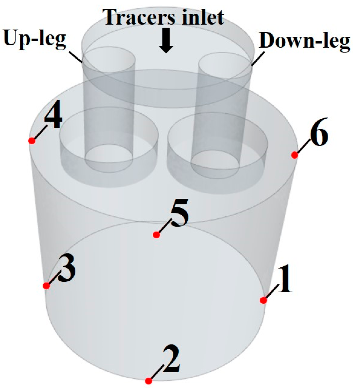
2.1. Physical Model

In this study, a water model with a similarity ratio of 1:4 was established based on a 260 t RH vacuum refining degasser from a factory, as shown in Figure 1. The dimensional parameters of the prototype and the water model are presented in

Table 2. Size parameters of industrial prototype and water model.

Parameters	Industrial Prototype	Water Model
Inner Diameter of Ladle Top (mm)	3912	978
Inner Diameter of Ladle Bottom (mm)	3716	929
Ladle Height (mm)	4140	1035
Inner Diameter of Vacuum Chamber (mm)	2298	574.5
Outer Diameter of Snorkel (mm)	1440	360
Inner Diameter of Snorkel (mm)	720	180
Length of Snorkel (mm)	1650	412.5
Inner Diameter of Gas Injection Orifices (mm)	8	2
Number of Gas Injection Orifices	16	16

. The water model is mainly made of acrylic glass, and other equipment includes a steel support frame, vacuum pump, gas compressor, rubber tubing, U-tube manometer, etc. Inside the up snorkel, there are 16 gas injection orifices arranged in two staggered rows, as shown in Figure 2. Water is used to simulate molten steel, and compressed air is used to simulate argon gas for the physical simulation experiments. The main physical parameters are shown in

Table 3. Main physical parameters.

Materials	ρ/(kg·m−3)	μ/(Pa·s)	Working Temperature/K	Lifting Gas Pressure/MPa
Air	1.184	1.86 × 10−5	298	0.6
Argon Gas	1.782	2.22 × 10−5	298	2.5
Molten Steel	7000	6.1 × 10−3	1873	-
Water	1000	0.89 × 10−3	298	-

.

In the refining process of the RH refining degasser, the flow of fluid is primarily affected by inertia force, gravity force, and viscous force. The dynamic similarity between the industrial and water models is satisfied by ensuring equal Froude numbers. Henceforth, it can be inferred that a correlation exists between the lifting gas flow rate in the water model and the actual RH lifting gas flow rate.

$$\frac{Q_m}{Q_p}=\sqrt{\frac{{\rho }_{g,p}}{{\rho }_{g,m}}\frac{\left({\rho }_{l,m}-{\rho }_{g,m}\right)}{\left({\rho }_{l,p}-{\rho }_{g,p}\right)}{\left(\frac{D_m}{D_p}\right)}^5}$$

(1)

where D is the geometric characteristic parameter, taking the inner diameter of the up snorkel, m; ${\rho }_g$ is the gas density, kg/m³; ${\rho }_l$ is liquid density, kg/m³. Subscripts m and p represent the water model and prototype, respectively.

The RH degasser is a reactor operating under vacuum cases, and it is crucial to ensure that the vacuum chamber pressure in the model closely matches that of the prototype. Based on geometric similarity, the water surface height of the vacuum chamber during the water model experiment and the liquid steel height in the prototype follow a similar ratio. According to the Bernoulli equation, a calculation formula is derived for determining the degree of vacuum in the water model.

$$\frac{\Delta P_m}{\Delta P_p}=\frac{P_0-P_m}{P_0-P_p}=\frac{{\rho }_m\mathrm{g}{H}_m}{{\rho }_p\mathrm{g}{H}_p}$$

(2)

where ΔP is the vacuum degree. H is the height difference between the liquid level in the vacuum chamber and the liquid level in the ladle, m.

2.2. Numerical Model

This model is established based on the dimensions of a water model and the Euler–Euler model is used to simulate the fluid flow within the RH. The model temporarily disregards the phenomena of heat transfer and chemical reactions within the degasser, focusing only on fluid flow. The free surface of the ladle top and the vacuum chamber are smooth and frictionless, without considering the presence of the slag layer. Air bubbles are assumed to be spherical, with their diameter set as a fixed value, and the average observed in experiments is 6 mm. The coalescence, collision, and breakup of bubbles are ignored. It is assumed that a solid wall is a no-slip boundary and that the wall function is applied in the near-wall region. The steady-state flow field is calculated in StarCCM+ software (17.02.007-R8), and based on the converged steady-state flow field, transient simulation calculations are carried out using pulse injection of tracer solution and passive scalars to study the flow field and tracer transport process. A passive scalar is a virtual tracer, which has no physical properties and only passively transports with the flow of water.

The Euler–Euler method solves conservation equations for each phase with its own velocity and physical properties coupled by interphase force. The volume fraction equation balances each phase’s volume in the fluid area.

Volume fraction equation: The balance of each phase in the fluid area is provided by its volume fraction. The volume of phase i is given by the following formula:

$$V_i={\displaystyle \underset{V}{\int }{\alpha }_i}dV$$

(3)

where α is the volume fraction of the phase, and i stands for gas or liquid phase. The volume fraction of each Euler phase must meet the following requirements.

$${\displaystyle \sum _{i=1}^n{\alpha }_i}=1$$

(4)

where n is the total number of phases.

Continuity equation: The mass conservation of phase i is given by the following formula:

$$\frac{\partial }{\partial t}\left({\rho }_i{\alpha }_i\right)+\nabla \cdot \left({\rho }_i{\alpha }_i{\mathbf{u}}_i\right)=0$$

(5)

where ρ is the density of the phase, kg/m³; u is the average velocity of the phase, m/s.

Momentum equation: The momentum conservation of phase i is given by the following formula:

$$\frac{\partial }{\partial t}\left({\alpha }_i{\rho }_i{\mathbf{u}}_i\right)+\nabla \cdot \left({\alpha }_i{\rho }_i{\mathbf{u}}_i{\mathbf{u}}_i\right)=-{\alpha }_i\nabla P+\nabla \cdot \left({\alpha }_i{\mu }_i^{eff}\left(\nabla {\mathbf{u}}_i+{\left(\nabla {\mathbf{u}}_i\right)}^T\right)\right)+{\alpha }_i{\rho }_i\overrightarrow{g}+{\overline{\mathrm{M}}}_i$$

(6)

$${\mu }_i^{eff}={\mu }_i+{\mu }_{t,i}$$

(7)

$\overrightarrow{g}$ is the vector of gravity acceleration, m/s²; P is the pressure shared by gas and liquid phases, Pa. ${\overline{\mathrm{M}}}_i$ is interphase force, N/m³. ${\mu }_i^{eff}$ is the effective viscosity, Pa·s, which consists of the dynamic viscosity of the phase ${\mu }_i$ and the turbulent viscosity of the phase ${\mu }_{t,i}$.

Interphase force: The momentum exchange term includes drag, virtual mass, lift, and turbulent dissipation forces.

$${\overline{M}}_i={\overline{M}}_l=-{\overline{M}}_g=F_D+F_{VM}+F_L+F_{TD}$$

(8)

Among them, subscripts l and g stand for the liquid phase and gas phase, respectively, and on the right, $F_L$ and $F_{TD}$ stand for drag force, virtual mass force, lift force, and turbulent dissipation force, respectively.

Drag force: The drag force model calculates the force exerted by the particles in the dispersed phase relative to the speed of the continuous phase. The drag model is a linear multiplier of the relative velocity of two phases. The following formula calculates the force acting on the gas phase by the liquid phase resistance.

$$F_D=A_D{\mathbf{u}}_r$$

(9)

$${\mathbf{u}}_r={\mathbf{u}}_g-{\mathbf{u}}_l$$

(10)

where $A_D$ is the linear drag coefficient and ${\mathbf{u}}_r$ is the relative velocity between two phases, m/s. Linearized drag coefficient is related to particle drag coefficient, and the formula is as follows:

$$A_D=C_D\frac{3{\alpha }_g{\alpha }_l{\rho }_l}{4d_g}\left|{\mathbf{u}}_r\right|$$

(11)

where d_g is the bubble diameter, m; $C_D$ is the drag coefficient. In relation (2–12) proposed by Schiller-Nauman [53], when Re_g > 1000, the value of the drag coefficient is 0.44. Where Re_g is the Reynolds number of the bubble.

$${\mathrm{Re}}_g=\frac{{\rho }_l{\mathbf{u}}_r{d}_g}{{\mu }_l}$$

(12)

Lift: When the flow field of the continuous phase is uneven or rotating, the discrete phase will be subjected to lift perpendicular to the velocity direction. The calculation formula is as follows:

$$F_L=C_L{\alpha }_g{\rho }_l\left[{\mathbf{u}}_r\times \left(\nabla \times {\mathbf{u}}_l\right)\right]$$

(13)

where $C_L$ is the lift coefficient. In this model, the lift coefficient of Auton is adopted [54], and the value is 0.5.

Virtual mass force: The virtual mass force acting on the gas phase by the acceleration of the gas relative to the liquid phase can be expressed by the following formula.

$$F_{VM}=C_{VM}{\rho }_l{\alpha }_g\left(a_g-a_l\right)$$

(14)

where $C_{VM}$ is the virtual mass coefficient, $a_l$ and $a_g$ are the acceleration of gas and liquid, m/s², respectively.

Turbulence dissipation force: The influence of turbulence on the redistribution of phase concentration inhomogeneity is simulated by adding turbulence dissipation force to the phase momentum equation in the following form:

$$F_{TD}=A_D{\mathbf{u}}_{TD}$$

(15)

$${\mathbf{u}}_{TD}=D_{TD}\cdot \left\{\frac{\nabla {\alpha }_g}{{\alpha }_g}-\frac{\nabla {\alpha }_l}{{\alpha }_l}\right\}$$

(16)

where ${\mathbf{u}}_{TD}$ is a relative drift velocity defined by volume fraction weighting, m/s; D_TD is the tensor transport coefficient.

2.2.1. Turbulence Model

The two-layer k-ε model combines the realizable k-ε model and the two-layer method [55,56]. The achievable k-ε model contains a new transfer equation of turbulence dissipation rate ε [55]. The two-layer method first proposed by Rodi is an alternative to the low Reynolds number method, which allows the k-ε model to be applied to layers affected by viscosity (including the viscous bottom layer and buffer layer) [56]. The transfer equations of turbulent kinetic energy k and turbulent dissipation rate ε are as follows:

$$\frac{\partial }{\partial t}\left({\rho }_i{k}_i\right)+\nabla \cdot \left({\rho }_i{k}_i{\mathbf{u}}_i\right)=\nabla \cdot \left[\left({\mu }_i+\frac{{\mu }_{t,i}}{{\sigma }_k}\right)\nabla k_i\right]+P_{k,i}-{\rho }_i{\epsilon }_i$$

(17)

$$\frac{\partial }{\partial t}\left({\rho }_i{\epsilon }_i\right)+\nabla \cdot \left({\rho }_i{\epsilon }_i{\mathbf{u}}_i\right)=\nabla \cdot \left[\left({\mu }_i+\frac{{\mu }_{t,i}}{{\sigma }_{\epsilon }}\right)\nabla {\epsilon }_i\right]+\frac{{\epsilon }_i}{k_i}{C}_{\epsilon 1}{P}_{\epsilon ,i}-C_{\epsilon 2}{\rho }_i\frac{{\epsilon }_i^2}{k_i}$$

(18)

where P_k,i and P_ε,i are the generating terms of phase i, which depends on the k-ε model. σ_k, σ_ε, C_ε1, and C_ε2 are model coefficients with values of 1, 1.2, 1.44, and 1.9, respectively. For the two-layer model, the turbulent dissipation rate ε near the wall can be simply expressed as the following formula:

$${\epsilon }_i=\frac{k_i^{3/2}}{l_{\epsilon ,i}}$$

(19)

where l_ε,i is the length scale function of phase i.

2.2.2. Tracer Transport Model

The tracer transport model includes a multicomponent fluid model and a passive scalar transport model. The multicomponent fluid model is used to predict the transport process of tracers in water. The model is described as follows:

$$\frac{\partial }{\partial t}\left({\rho }_l{W}_T\right)+\nabla \cdot \left({\rho }_l{\mathbf{u}}_l{W}_T\right)=\nabla \cdot \left({\rho }_l{D}_{eff}\nabla W_T\right)$$

(20)

where W_T is the mass fraction of water and tracer, respectively. When tracers are injected into the top entrance of the water model, W_T = 1. When the injection of tracers is stopped, W_T = 0. The effective transport coefficient D_eff is the sum of the molecular transport coefficient and turbulent transport coefficient, as follows:

$$D_{eff}=D_l+D_{t,l}$$

(21)

where D_l is the molecular transport coefficient of the liquid phase and D_t,l is the turbulent transport coefficient. The density of the mixing fluid in all the continuity, momentum, and turbulence equations are calculated as follows:

$$\frac{1}{{\rho }_l}=\left(1-W_T\right)\frac{1}{{\rho }_w}+W_T\frac{1}{{\rho }_T}$$

(22)

where ρ_w and ρ_T are the density of water and tracer, respectively.

The passive scalar transport model is used to predict the transport process of the passive scalar. The description is as follows:

$$\frac{\partial }{\partial t}\left({\rho }_l{W}_S\right)+\nabla \cdot \left({\rho }_l{\mathbf{u}}_l{W}_S\right)=\nabla \cdot \left({\rho }_l{D}_{eff}\nabla W_S\right)$$

(23)

where W_S is the mass fraction of the passive scalar.

2.2.3. Mesh and Boundary Conditions

In this study, a 3D model of RH water model is established, and polyhedral mesh is used for simulation. The gas injection orifices and tracer addition locations are encrypted, as shown in Figure 3.

The ladle wall, snorkel, and vacuum chamber are set to no-slip boundary conditions and treated with wall function in the area near the wall. The surface of the ladle and vacuum chamber is treated with a phase permeability condition that allows bubbles to escape from the surface while preventing the liquid phase from penetrating. The inlet velocity of a single gas injection orifice is calculated from the total gas flow rate. At the location of the gas injection orifice, the volume fraction of water is set to 0. The turbulent kinetic energy and turbulent dissipation rate at the inlet were calculated using the method proposed by Ilegbusi et al. [57].

$$k=0.015{{\overrightarrow{u}}_g}^2$$

(24)

$$\epsilon =\frac{47k^{1.5}}{r_n}$$

(25)

where r_n represents the radius of the orifice, m.

2.3. Studied Cases

This study devised three schemes under two lifting gas flow rates (20 L/min and 40 L/min), as shown in

Table 4. Dosage and the kind of tracer.

Materials	Cass 1	Cass 2	Cass 3
Tracer Dosage/mL	300	300	600
Tracer Kind	NaCl solution	Passive scalar	NaCl solution

. By conducting numerical calculations and water model experiments to monitor the changes in conductivity at six points inside the ladle, it compared the differences in the transport processes of various types and doses of tracers. Figure 4 is a schematic diagram of the tracer injection location and monitoring points. The tracer is introduced through the central entrance at the top of the vacuum chamber. Six monitoring points are arranged inside the ladle. Monitoring points 1–3 are located at the bottom of the ladle, while monitoring points 4–6 are situated 50 mm below the liquid surface at the top of the ladle.

3. Results

3.1. Model Verification

When the lifting gas flow rate is 40 L/min and the dosage of NaCl solution is 300 mL, the dimensionless concentration–time curves at monitoring points 1 and 2 at the bottom of the ladle are shown in Figure 5. It can be observed that the predicted curve from the numerical simulation aligns very well with the experimental data. At monitoring point 1, the peak of the prediction curve is 11.1, and the maximum peak of experimental results is 10. The difference between the maximum peaks is 1.1. At monitoring point 2, the peak of the prediction curve is 7.2, the maximum peak of experimental results is 8.1, and thus the difference between the maximum peaks is 0.9. It indicates that the mathematical model used in this paper can accurately predict the fluid flow and tracer transport process in the RH water model.

3.2. Flow Pattern

When the lifting gas flow rate is 40 L/min, the predicted flow field results of the RH water model are shown in Figure 6. Inside the ladle, there are two circulation zones, one larger and one smaller, on the left and right sides, respectively. Observing the velocity distribution in the flow field, the water flow speed is higher in the active areas such as the up snorkel, vacuum chamber, down snorkel, and the impact zone of the descending flow. Conversely, the water flow speed in other areas inside the ladle is relatively lower.

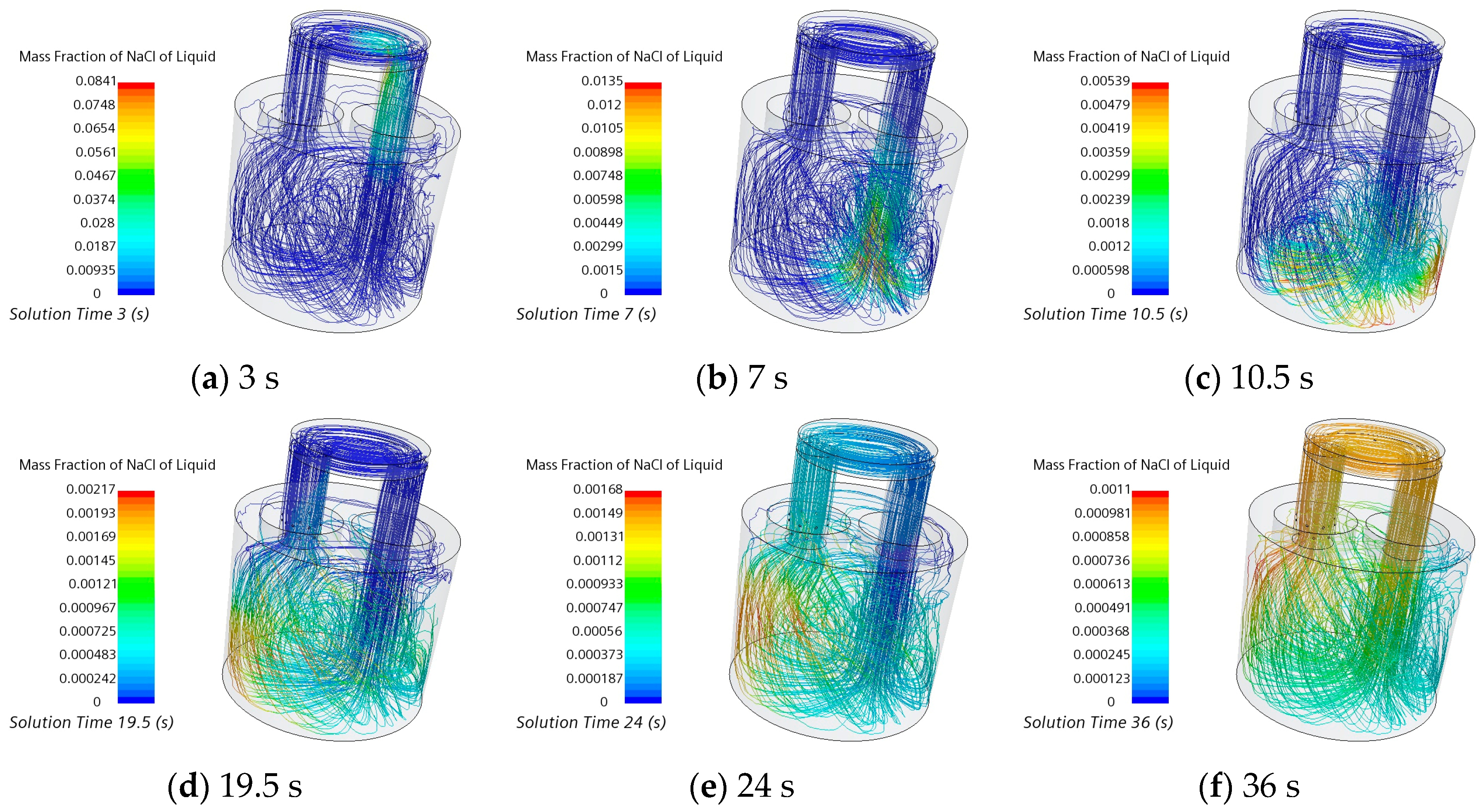
3.3. Transport Process of Salt Tracer

When the lifting gas flow rate is 40 L/min, and the additional dosage of NaCl solution is 300 mL, the tracer transport process added from the central entrance at the top of the vacuum chamber is shown in Figure 7. As seen from Figure 7a–c, after the tracer is added from the central entrance at the top of the vacuum chamber, it will disperse to the down snorkel side with the circulation in the vacuum chamber. After entering the down snorkel, the tracer will continue to move downward and spread around after contacting the bottom of the ladle. As shown in Figure 7d–f, the tracer will move upward with the circulation after spreading at the bottom of the ladle. With the significant circulation movement on the left, part of the tracer will enter the up snorkel. Driven by the lifting gas, this part of the tracer will enter the vacuum chamber through the up snorkel and continue to move, thus starting the next round of the circulation process. As shown in Figure 7g, at 51 s, a large number of tracers are concentrated in the down snorkel, indicating that after the tracer is added, the first round of circulation between the vacuum chamber and the ladle has ended. Then, similar to the first round of the circulation process, the tracer will be continuously circulated in the RH water model under the action of circulation. As shown in Figure 7h, at 77 s, the interior of the RH water model has been filled with the tracer in a nearly uniform state. With the continuous mixing, at 100 s, the tracer concentration in the model has not changed, indicating that the mixing state has been reached, as shown in Figure 7i.

3.4. Comparison of Tracer Transport Processes with Different Densities

3.4.1. Comparison of Tracer Transport Processes with Different Densities When the Lifting Gas Flow Rate Is 40 L/min

When the lifting gas flow rate is 40 L/min, and the dosage of passive scalar and NaCl solution is the same, Figure 8 illustrates the transport process of the tracer in the main cross-section of the RH water model. From Figure 8(a1–c1) or Figure 8(a2–c2), it can be observed that after diffusing into the interior of the ladle, the tracer splits into two streams due to the circulation, continuing to spread on both the left and right sides of the ladle’s bottom. At 10.3 s, the concentration area of the tracer under the NaCl solution case is concentrated on the right wall of the ladle, while under the passive scalar case, the concentration area of the tracer remains on the right side of the ladle’s bottom, as shown in Figure 8(b1,b2). It is evident that at 15 s, compared to the passive scalar case, the concentration area of the tracer under the NaCl solution case is closer to the left side of the ladle’s bottom, as illustrated in Figure 8(c1,c2). In other words, the transport rate of the salt tracer within the ladle is faster.

In this case, the tracer transport process on the side section of the RH water model is shown in Figure 9. From Figure 9(a1–c1) or Figure 9(a2–c2), it can be observed that on the side section of the ladle, the tracer first transports towards the bottom of the ladle, then to the bottom sidewall, and, finally, continues to transport upwards along the ladle sidewall. At 15 s, the concentration area of the tracer under the NaCl solution case has already approached the bottom of the ladle, while the concentration area of the tracer under the passive scalar case is still located on both sides of the ladle bottom, as shown in Figure 9(c1,c2). In other words, the transport rate of salt tracers on the ladle side section is faster.

The dimensionless concentration–time curves at monitoring points 1–3 at the bottom of the ladle are shown in Figure 10. At monitoring points 1 and 2 below the down snorkel, compared to the curve of the passive scalar, the curve of the NaCl solution shifts to the left, but the extent is small. At the monitoring point, the farthest from the down snorkel, the curve of the NaCl solution shows a significant leftward shift compared to that of the passive scalar. This is because the density of the NaCl solution is higher than that of water, and the passive scalar, as a virtual tracer, can only move with the water flow, resulting in faster transport of the NaCl solution to the bottom of the ladle (the density effect).

The tracer transport process at the bottom of the ladle is shown in Figure 11. From Figure 11(a1–c1) or Figure 11(a2–c2), it can be observed that at the bottom of the ladle, the tracer gradually transports from the right side (below the down snorkel) to the left side (below the up snorkel) and eventually fills the entire bottom area. At monitoring point 3 (located on the left side of the ladle bottom), the mass fraction of the tracer is higher, and this area is referred to as the “inactive zone”. At 10.1 s and 12.02 s, the concentration area of the tracer in the NaCl solution case is closer to the left side of the ladle bottom (monitoring point 3) compared to the passive scalar case, indicating that the saltwater tracer transports faster at the bottom of the ladle, as shown in Figure 11(a1,b1,a2,b2). Additionally, at monitoring point 3, the concentration of the tracer in the NaCl solution case is higher than that in the passive scalar case, as shown in Figure 11(c1,c2). This corresponds to the peak of the concentration–time curve of the NaCl solution in Figure 10c being higher than that of the passive scalar case.

The upward tracer transport process on the main section of the RH water model is shown in Figure 12. At 45 s, near the liquid surface of the ladle close to the up snorkel (monitoring point 4), the concentration of the tracer in the NaCl solution case is higher than that in the passive scalar case. Meanwhile, near the liquid surface of the ladle close to the down snorkel (monitoring point 6), the concentration of the tracer in the passive scalar case is higher than that in the NaCl solution case, as shown in Figure 12(b1,b2). The situation remains similar at 75 s, as shown in Figure 12(c1,c2). Therefore, it can be concluded that the transport rate of the salt tracer is faster on the left side of the top of the ladle (monitoring point 4), while the transport rate of the passive scalar is faster on the right side of the top of the ladle (monitoring point 6).

Figure 13 shows the dimensionless concentration–time curves at monitoring points 4–6 on the top of the ladle. At monitoring point 4, which is on the left side of the up snorkel, the curve of the NaCl solution shifts to the left relative to that of the passive scalar, as shown in Figure 13a. At monitoring point 5, there is almost no difference between the curve of the NaCl solution and that of the passive scalar, but the peak of the passive scalar’s curve is higher, as shown in Figure 13b. At monitoring point 6, which is on the right side of the down snorkel, the curve of the NaCl solution shifts to the right relative to that of the passive scalar, as shown in Figure 13c.

Overall, the tracer transport process to the top area of the ladle goes through two stages: (1) When the tracer is carried to the bottom of the ladle with the circulation, the higher density of the salt tracer compared to the passive scalar causes density and gravity to promote transport, making the transport rate of the salt tracer faster. (2) As the tracer continues to transport upwards to the top of the ladle, density and gravity hinder its transport, slowing down the transport rate of the saltwater tracer, with different effects of density and gravity in the two stages. In the large circulation area on the left side of the ladle, the promotion to transport of the salt tracer is greater than the hindrance, resulting in a faster concentration growth rate at monitoring point 4 compared to the passive scalar. In the circulation area on the right side of the ladle, the hindrance to the transport of the salt tracer is greater than the promotion, leading to a slightly slower concentration growth rate at monitoring point 6 compared to the passive scalar. In the area below monitoring point 5, the promoting and hindering effects are roughly equal, resulting in the same concentration growth rate for the saltwater tracer and passive scalar at that point.

3.4.2. Comparison of Different Tracer Transport Processes When the Lifting Gas Flow Rate Is 20 L/min

Figure 14 shows the transport process of the tracer on the main cross-section of the RH water model with the lifting gas flow rate of 20 L/min and the addition of 300 mL of passive scalar and 300 mL or 600 mL of NaCl solution, respectively. Similar to the case with a lifting gas flow rate of 40 L/min, the tracer continues to transport to the bottom of the ladle after passing through the down snorkel and then transports to the left and right side walls of the ladle. At 10.3 s, the concentrated areas of tracer concentration in the passive scalar case have not yet reached the bottom of the ladle, while in both the 300 mL NaCl solution and 600 mL NaCl solution cases, the concentrated areas of tracer concentration have already reached the bottom of the ladle. Furthermore, the concentrated areas of tracer concentration in the 600 mL NaCl solution case are noticeably larger than that in the 300 mL NaCl solution case, which may be due to the different amounts of tracer added, as shown in Figure 14(b1–b3). At 15 s, the concentrated areas of tracer concentration in the NaCl solution cases have already reached monitoring point 1 (the right side of the bottom of the ladle), while, in the passive scalar case, this area has not yet been reached, as shown in Figure 14(c1–c3). Therefore, it can be observed that the transport rate of salt tracers within the ladle is still faster.

Figure 15 illustrates the transport process of the tracer on the side cross-section of the RH water model. Similar to the case with a lifting gas flow rate of 40 L/min, the tracer first transports downwards on the side cross-section of the ladle and then transports towards the left and right side walls. At 10.1 s, in the passive scalar case, the concentrated area of tracer concentration has not yet reached the bottom of the ladle, whereas in both the 300 mL NaCl solution and 600 mL NaCl solution cases, the concentrated areas of tracer concentration have already reached the bottom of the ladle, as shown in Figure 15(b1–b3). At 15 s, in the passive scalar case, the concentrated area of tracer concentration is located at the center of the bottom of the ladle; in the 300 mL NaCl solution case, the concentrated area of tracer concentration is near both sides of the bottom of the ladle; and in the 600 mL NaCl solution case, the concentrated area of tracer concentration is already at both sides of the bottom of the ladle, as shown in Figure 15(c1–c3). This indicates that the transport rate of salt tracers on the side cross-section of the ladle is still faster and that the 600 mL NaCl solution exhibits a faster transport rate compared to the 300 mL NaCl solution.

Figure 16 shows the dimensionless concentration–time curves at monitoring points 1–3 at the bottom of the ladle. At monitoring points 1 and 2, located below the down snorkel, the curve of the NaCl solution is significantly shifted to the left and has a higher concentration compared to the passive scalar’s curve. Additionally, when comparing the 600 mL NaCl solution to the 300 mL NaCl solution, there is also a leftward shift in the curve, as shown in Figure 16a,b. The curve of the saltwater tracer exhibits a clear leftward shift compared to the passive scalar; similarly, there is a significant leftward shift in the curve when comparing the 600 mL NaCl solution to the 300 mL NaCl solution, as illustrated in Figure 16c. Therefore, it can be deduced that due to the density effect within the ladle, the NaCl solution can transport more quickly to the bottom, and this effect becomes more pronounced with an increased amount of NaCl solution added.

The transport process of the tracer at the bottom of the ladle is shown in Figure 17. At 10.1 s, the concentration area of the tracer under the NaCl solution case is significantly higher than that under the passive scalar case, as shown in Figure 17(a1–a3). At 18 s, the concentrated area of the tracer under the NaCl solution case is located on the right side of the bottom of the ladle (at monitoring point 1), while the concentrated area of the tracer under the passive scalar case is still at the center of the bottom of the ladle, as illustrated in Figure 17(b1–b3). Additionally, at 35.01 s, the concentrated area of the tracer for both the passive scalar and saltwater tracer cases is located on the left side of the bottom of the ladle (at monitoring point 3), as shown in Figure 17(c1–c3). Specifically, on the left side of the bottom of the ladle, the tracer mass fraction is highest in the 600 mL NaCl solution case, followed by the 300 mL NaCl solution case, and is lowest in the passive scalar case. This corresponds to Figure 16c, where it can be observed that the peak of the dimensionless concentration curve of the NaCl solution is higher than that of the passive scalar, and the peak of the 600 mL NaCl solution is higher than that of the 300 mL NaCl solution.

The upward transport process of the tracer on the main section of the RH water model is shown in Figure 18. Similar to the case with the lifting gas flow rate of 40 L/min, at 45 s, in the area near the liquid surface of the ladle close to the up snorkel (monitoring point 4), the tracer concentration in the NaCl solution case is higher than that in the passive scalar case. However, in the area near the liquid surface of the ladle close to the down snorkel (monitoring point 6), the tracer concentration in the passive scalar case is higher than that in the NaCl solution case. At 75 s, in the area near the liquid surface of the ladle close to the down snorkel (monitoring point 6), the tracer concentration is highest in the passive scalar case, followed by the 300 mL NaCl solution, and the 600 mL NaCl solution has the lowest concentration. Therefore, on the left side of the top of the ladle (monitoring point 4), the saltwater tracer still has a faster transport rate, while on the right side of the top of the ladle (monitoring point 6), the passive scalar still has a faster transport rate. Additionally, in that area (monitoring point 6), the 300 mL NaCl solution has a faster transport rate than the 600 mL NaCl solution.

Figure 19 shows the dimensionless concentration–time curves at monitoring points 4–6 on the top of the ladle. At monitoring point 4, located on the left side of the up snorkel, the curve of the NaCl solution shifts noticeably to the left compared to the passive scalar solution, with little difference in the degree of leftward shift between the 600 mL and 300 mL NaCl solution cases, as shown in Figure 19a. At monitoring point 5, the curve of the 300 mL NaCl solution nearly overlaps with that of the passive scalar, while the peak of the curve of the 600 mL NaCl solution is lower, as shown in Figure 19b. At monitoring point 6, on the right side of the down snorkel, the curves of the NaCl solution shift noticeably to the right compared to the passive scalar, and the shift is greater for the 600 mL NaCl solution than for the 300 mL solution, as shown in Figure 19c. Similar to the case with the lifting gas flow rate of 40 L/min, in the large recirculation zone on the left side of the ladle, the promoting effect of the saltwater tracer is greater than the hindering effect, leading to a faster rate of concentration increase; in the recirculation zone on the right side of the ladle, the promoting effect is less than the hindering effect, resulting in a slower rate of concentration increase, and the hindering effect increases with the dose of the tracer. Similarly, below monitoring point 5, the two effects on the saltwater tracer nearly cancel each other out, having no impact on the rate of increase.

Figure 20 compares the experimental data and numerical prediction results of the dimensionless concentration–time curves at monitoring points 4–6 on the top of the ladle. In this case, the numerical simulation represents the curves of the passive scalar, and the experimental data are the averaged dimensionless concentration curves obtained from ten repeated experiments with 300 mL and 600 mL NaCl solutions. At monitoring point 4, located on the left side of the up snorkel, the NaCl solution shifts to the right relative to the passive scalar and exhibits a higher peak, as shown in Figure 20a. At monitoring point 5, the NaCl solution also shifts to the right relative to the passive scalar, and the shift is more pronounced for the 600 mL NaCl solution, as shown in Figure 20b. At monitoring point 6, on the right side of the down snorkel, the 300 mL NaCl solution nearly overlaps with the passive scalar. In contrast, the 600 mL NaCl solution shows a gradual increase to a stable state after a slow rising step, as shown in Figure 20c.

Figure 21 compares the experimental data and numerical prediction results of the dimensionless concentration–time curves at monitoring point 3. The curve of 600 mL NaCl solution slowly declines after the peak, which is different from the curve in other cases. This suggests that in this case, when the salt solution impacts the bottom of the ladle, some of the salt may deposit at the corners on the left side of the ladle bottom, as shown in Figure 21b, and then slowly move upward in the ladle.

At monitoring point 4, the experimental concentration–time curve of the NaCl solution shifts to the right relative to the curve of the passive scalar. However, the predicted curve for the NaCl solution shifts to the left relative to the passive scalar’s curve. As for monitoring points 5 and 6, both the experimental and predicted curves of the NaCl solution shift to the right relative to the passive scalar’s curves, but their trends are not completely consistent. This indicates that the mathematical model may have certain limitations in predicting the outcomes in this area.

3.4.3. Comparison of Mixing Time

Under the case of lifting gas flow rate at 40 L/min, based on the 95% standard,

Table 5. The mixing time of monitoring points 1–6 and the lifting gas flow rate is 40 L/min.

	Point 1	Point 2	Point 3	Point 4	Point 5	Point 6
Passive scalar (numerical prediction)	60.9	65.26	74.95	69.65	64.78	69.25
NaCl solution (numerical prediction)	59.62	64.1	74.65	88.48	62.98	88.48
NaCl solution (experimental data)	83.9	79.3	81.5	101	101	91

shows the mixing times at monitoring points 1–6. In both cases, the amount of passive scalar and NaCl solution added was 300 mL. For the NaCl solution case, the experimental mixing times were calculated by excluding the maximum and minimum values from ten repeated experiments and taking the average value as the result. From the table, it can be seen that, in terms of numerical prediction and physical experiment of salt tracers, the mixing time at the top of the ladle (monitoring points 4–6) is generally higher than at the bottom (monitoring points 1–3). According to the prediction results, at the bottom of the ladle (monitoring points 1–3), the difference in mixing time between the passive scalar case and the NaCl solution case is not significant. However, at the top of the ladle, except for monitoring point 5, the mixing time under the NaCl solution case is significantly longer than that under the passive scalar case (for example, at monitoring point 4, the mixing time for the passive scalar case is 18.83 s shorter than for the NaCl solution case, with a difference of 27%. For monitoring point 6, the mixing time for the passive scalar case is 19.23 s shorter than for the NaCl solution case, with a difference of 27.8%. Additionally, the experimental values of mixing time under the NaCl solution case are usually longer than the predicted results. This may be due to a certain range of errors inherent in the conductivity probes used in the experiments.

When the lifting gas flow rate is 20 L/min, the mixing time of monitoring points 1–6 under the 95% standard is shown in

Table 6. The mixing time of monitoring points 1–6 and the lifting gas flow rate is 20 L/min.

	Point 1	Point 2	Point 3	Point 4	Point 5	Point 6
300 mL Passive scalar (numerical prediction)	73.7	75.7	66.18	86.02	79.54	75.6
300 mL NaCl solution (numerical prediction)	71.65	74	69.5	92.05	81.82	86.68
600 mL NaCl solution (numerical prediction)	73.2	75.1	81.16	100.75	74	106.69
300 mL NaCl solution (experimental data)	111	102	116	127	122	130
600 mL NaCl solution (experimental data)	109	118	108	131	134	143

. Among them, the dosage of passive scalar is 300 mL, and the dosage of NaCl solution is 300 mL and 600 mL. Similar to the case with the lifting gas flow rate of 40 L/min, it can be seen from numerical prediction and physical experiments that the mixing time at the top of the ladle (monitoring points 4–6) is generally higher than that at the bottom of the ladle (monitoring points 1–3). This indicates that the tracer first diffuses downwards to the bottom of the ladle and then upwards to the top, thereby prolonging the mixing time. According to the numerical simulation results, for monitoring point 1, the mixing time of the NaCl solution case is 2.05 s shorter than that of the passive scalar, with a difference of 3%. When the dosage of NaCl solution is increased to 600 mL, the difference is reduced to less than 1%. For monitoring point 2, the mixing time of the NaCl solution case is 1.7 s shorter than that of the passive scalar, with a difference of 2%. Similarly to monitoring point 1, when the dosage of NaCl solution is increased to 600 mL, the difference is reduced to less than 1%. For monitoring point 3, the mixing time of the NaCl solution case is 3.3 s delayed than that of the passive scalar, with a difference of 5%. When the dosage of NaCl solution is increased to 600 mL, the mixing time is delayed by about 15 s more than that of the passive scalar, and the difference is increased to 22.6%. For monitoring point 4, the mixing time of the NaCl solution case is 6 s delayed than that of the passive scalar, with a difference of 7%. When the dosage of NaCl solution is increased to 600 mL, the difference is 14 s with an increasing ratio of 17.1%. For monitoring point 5, the mixing time of the NaCl solution case is 2.3 s delayed compared to that of the passive scalar, with a difference of 3%. When the dosage of NaCl solution is increased to 600 mL, the mixing time of the NaCl solution case is 5.5 s shorter than that of the passive scalar, with a difference of 7%. For monitoring point 6, the mixing time of the NaCl solution case is 11.1 s more delayed than that of the passive scalar, with a difference of 14.7%. When the dosage of NaCl solution is increased to 600 mL, the difference is 31 s and the increasing ratio is increased to 41.1%.

According to the experimental data, the mixing time is obviously greater than that of the numerical simulation result. Compared with the cases of 300 mL NaCl solution and 600 mL NaCl solution, for monitoring points 1 and 3, the mixing time is 2 s and 8 s shortened, respectively, by increasing dosage. For monitoring point 2, the mixing time is 14 s delayed when increasing the dosage of the tracer. For monitoring points 4, 5, and 6, the mixing time is 4 s, 12 s, and 13 s delayed, respectively, by increasing the dosage of the tracer.

When the lifting gas flow rate is 40 L/min and 20 L/min, the mixing time of the passive scalar case and NaCl solution case is not obvious at monitoring points 1, 2, and 3, with a difference of 1–5%. When the lifting gas flow rate is 40 L/min, for monitoring points 4 and 6, the mixing time of the NaCl solution case is more delayed than that of the passive scalar, with a difference of 27%. For monitoring point 5, the mixing time of the NaCl solution case is slightly shorter than that of the passive scalar, and the difference is 2.8%. When the lifting gas flow rate is 20 L/min and the dosage of NaCl solution is increased to 600 mL, the difference is reduced to less than 1% at monitoring points 1 and 2, but for monitoring point 3, the difference is increased to 22.6%. For monitoring points 4, 5, and 6, the mixing time of the NaCl solution case is more delayed than that of the passive scalar, with a difference of 3–14.7%. When the dosage of NaCl solution is increased to 600 mL, the difference is increased to 17.1–41.1% at monitoring points 4 and 6. The results of numerical simulation and physical experiment of salt tracers show that the mixing time will increase at the top of the ladle (monitoring points 4 and 6) when the tracer dosage is increased from 300 mL to 600 mL.

4. Conclusions

Based on 260 t RH, a water model with a similarity ratio of 1:4 was established, the transport process of the passive scalar tracer (virtual tracer) and NaCl solution tracer (considering density effect) was numerically simulated under two lifting gas flow rates, and the following conclusions were made:

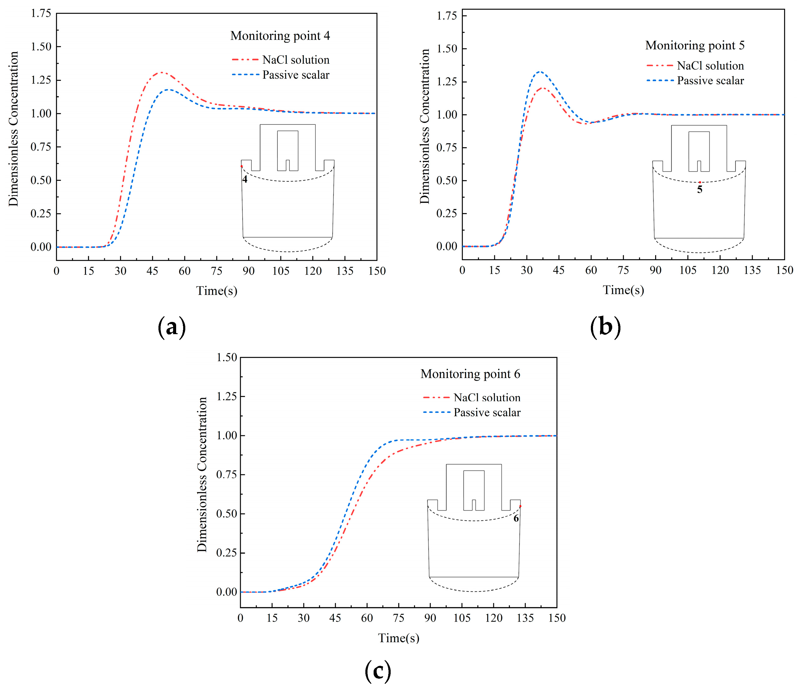
• Under both gas lifting flow rates, the transport rate of the NaCl solution tracer into the ladle is faster, and its transport rate at the bottom of the ladle is also faster than that of the passive scalar tracer. In the area near the up snorkel at the top of the ladle, the transport rate of the NaCl solution tracer remains faster. In the area near the down snorkel at the top of the ladle, the transport rate of the passive scalar is faster.
• The transport of the tracer to the top region of the ladle involves two stages: (1) When the tracer is carried to the bottom of the ladle with the recirculation, at this point, because the density of the salt tracer is higher than that of the passive scalar, density and gravity promote the transport of the tracer, making the transport rate of the salt tracer faster. (2) As the tracer continues to diffuse upwards to the top of the ladle, density and gravity hinder the transport of the tracer, slowing down the transport rate of the salt tracer, with density and gravity playing different roles in the two stages. Due to the different flow field structures inside the ladle, the degree of promotion and obstruction of density and gravity is also different. In the large circulation area on the left side of the ladle, the promoting effect is greater than the hindering effect. Therefore, in the left area at the top of the ladle, the concentration of salt tracer increases faster than that of the passive scalar. In the small circulation flow area on the right side of the ladle, the hindering effect is greater than the promoting effect, resulting in a slower increase in the concentration of salt tracer in the top right area of the ladle compared to the passive scalar. In the middle area of the ladle, the promoting and hindering effects are the same, and the concentration growth rate of the salt tracer is the same as that of the passive scalar.
• For both gas lifting flow rate cases, the mixing time at the top of the ladle is generally higher than that at the bottom. When comparing the mixing time at the top and bottom of the ladle, the difference in the passive scalar case is 1.3% and 11.8% for 40 L/min and 20 L/min flow rate schemes, respectively. In addition, the difference of the NaCl solution case (300 mL) increases to 21% and 21.2% for the two flow rate schemes. In the case of 600 mL NaCl solution, this difference increases to 19.7% and 22.6% for the two schemes.
• When comparing the mixing time between the passive scalar and NaCl solution tracer, at the bottom of the ladle, the difference in mixing time between the passive scalar case and the NaCl solution case is not significant, within the difference range between 1 and 5%. However, at the top of the ladle, the mixing time for the NaCl solution case is significantly longer than that for the passive scalar case, with the difference range between 3 and 14.7%. The increase in the dosage of tracer increases the difference to 17.4–41.1%. This indicates that density and gravity delay the mixing of substances in the top area of the ladle. In the industrial refining process, when adding denser alloys, attention should be paid to the mixing of substances in the top area of the ladle.

References

1. Zhang, L.F.; Peng, K.Y.; Ren, Y. Kinetic Analysis for Steel Desulfurization during Ruhrstahl–Heraeus Process. Steel Res. Int. 2023, 95, 2300399. [Google Scholar] [CrossRef]
2. She, C.J.; Peng, K.Y.; Sun, Y.; Ren, Y.; Zhang, L.F. Kinetic Model of Desulfurization during RH Refining Process. Metall. Mater. Trans. B 2024, 55, 92–104. [Google Scholar] [CrossRef]
3. Wang, H.J.; Xu, R.; Ling, H.T.; Zhong, W.; Chang, L.Z.; Qiu, S.T. Numerical simulation of fluid flow and alloy melting in RH process for electrical steels. J. Iron Steel Res. Int. 2022, 29, 1423–1433. [Google Scholar] [CrossRef]
4. Liu, C.; Peng, K.Y.; Wang, Q.; Li, G.Q.; Wang, J.J.; Zhang, L.F. CFD Investigation of Melting Behaviors of Two Alloy Particles during Multiphase Vacuum Refining Process. Metall. Mater. Trans. B 2023, 54, 2174–2187. [Google Scholar] [CrossRef]
5. Kim, T.S.; Yang, J.; Park, J.H. Effect of Physicochemical Properties of Slag on the Removal Rate of Alumina Inclusions in the Ruhrstahl–Heraeus (RH) Refining Conditions. Metall. Mater. Trans. B 2022, 53, 2523–2533. [Google Scholar] [CrossRef]
6. Zhong, H.J.; Jiang, M.; Wang, Z.Y.; Zhen, X.G.; Zhao, H.M.; Li, T.G.; Wang, X.H. Formation and Evolution of Inclusions in AH36 Steel during LF–RH–CC Process: The Influences of Ca-Treatment, Reoxidation, and Solidification. Metall. Mater. Trans. B 2023, 54, 593–601. [Google Scholar] [CrossRef]
7. Peng, K.Y.; Wang, J.J.; Li, Q.L.; Liu, C.; Zhang, L.F. Multiphase Simulation on the Collision, Transport, and Removal of Non-metallic Inclusions in the Molten Steel during RH Refining. Metall. Mater. Trans. B 2023, 54, 928–943. [Google Scholar] [CrossRef]
8. Zhang, S.; Liu, J.H.; He, Y.; Zhou, C.H.; Yuan, B.H.; Zhang, M.; Barati, M. Study of Dispersed Micro-Bubbles and Improved Inclusion Removal in Ruhrstahl–Heraeus (RH) Refining with Argon Injection through Down Leg. Metall. Mater. Trans. B 2023, 54, 2347–2359. [Google Scholar] [CrossRef]
9. Li, H.; Liu, J.X.; Ren, Q.; Zhang, L.F. Effect of Ruhrstahl Heraeus Refining Time on Inclusions and Rolling Contact Fatigue Life of a High-Carbon Chromium Bearing Steel. Steel Res. Int. 2023, 94, 2200977. [Google Scholar] [CrossRef]
10. Ramírez-López, A. Analysis of Mixing Efficiency in a Stirred Reactor Using Computational Fluid Dynamics. Symmetry 2024, 16, 237. [Google Scholar] [CrossRef]
11. He, Q.; Yao, T.L.; Liu, L.; Li, X.C.; Ni, B.; Li, L.F. An experimental study on RH vacuum chamber with a weir. J. Iron Steel Res. Int. 2023, 30, 1929–1938. [Google Scholar] [CrossRef]
12. Kato, Y.; Nakato, H.; Fujii, T.; Ohmiya, S.; Takatori, S. Fluid flow in ladle and its effect on decarburization rate in RH degasser. ISIJ Int. 1993, 33, 1088–1094. [Google Scholar] [CrossRef]
13. Yoshitomi, K.; Nagase, M.; Uddin, M.A.; Kato, Y. Fluid Mixing in Ladle of RH Degasser Induced by Down Flow. ISIJ Int. 2016, 56, 1119–1123. [Google Scholar] [CrossRef]
14. Zhang, L.F.; Li, F. Investigation on the Fluid Flow and Mixing Phenomena in a Ruhrstahl-Heraeus (RH) Steel Degasser Using Physical Modeling. JOM 2014, 66, 1227–1240. [Google Scholar] [CrossRef]
15. Liu, C.; Zhang, L.F.; Li, F.; Peng, K.Y.; Liu, F.G.; Liu, Z.T.; Zhao, Y.Y.; Yang, W.; Zhang, J. Water Modeling on Circulating Flow and Mixing Time in a Ruhrstahl–Heraeus Vacuum Degasser. Steel Res. Int. 2021, 92, 2000608. [Google Scholar] [CrossRef]
16. Wang, R.D.; Jin, Y.; Cui, H. The Flow Behavior of Molten Steel in an RH Degasser Under Different Ladle Bottom Stirring Processes. Metall. Mater. Trans. B 2022, 53, 342–351. [Google Scholar] [CrossRef]
17. Zhang, S.; Liu, J.H.; He, Y.; Zhou, C.H.; Yuan, B.H.; Mclean, A. Bubble formation by argon injection through the down-leg snorkel with Ruhrstahl-Heraeus (RH) circulating flow. J. Mater. Process. Technol. 2022, 306, 117647. [Google Scholar] [CrossRef]
18. Zhang, Z.M.; Ma, P.; Dong, J.H.; Liu, M.; Liu, Y.G.; Lai, C.B. Effects of Different RH Degasser Nozzle Layouts on the Circulating Flow Rate. Materials 2022, 15, 8476. [Google Scholar] [CrossRef]
19. Liu, Z.; Lou, W.; Zhu, M.Y. Numerical Analysis of Fluid Flow and Powder Transport Characteristics of RH-Degasser Ladle Bottom Powder Injection (RH-PBI) Process. Metall. Mater. Trans. B 2024, 55, 418–430. [Google Scholar] [CrossRef]
20. Chen, G.J.; He, S.P. Volume of fluid simulation of single argon bubble dynamics in liquid steel under RH vacuum conditions. J. Iron Steel Res. Int. 2024, 31, 828–837. [Google Scholar] [CrossRef]
21. Dong, W.L.; Xu, A.J.; Liu, B.S.; Zhou, H.C.; Ji, C.X.; Wang, S.J.; Li, H.B.; Wang, T.H. Mechanism and Model of Nitrogen Absorption of Molten Steel during N2 Injection Process in RH Vacuum. Metall. Mater. Trans. B 2024, 55, 72–82. [Google Scholar] [CrossRef]
22. Geng, D.Q.; Zhang, X.; Liu, X.A.; Wang, P.; Liu, H.T.; Chen, H.M.; Dai, C.M.; Lei, H.; He, J.C. Simulation on Flow Field and Mixing Phenomenon in Single Snorkel Vacuum Degasser. Steel Res. Int. 2015, 86, 724–731. [Google Scholar] [CrossRef]
23. Dong, J.F.; Feng, C.; Zhu, R.; Wei, G.S.; Jiang, J.J.; Chen, S.Z. Simulation and Application of Ruhrstahl–Heraeus (RH) Reactor with Bottom-Blowing. Metall. Mater. Trans. B 2021, 52, 2127–2138. [Google Scholar] [CrossRef]
24. Dong, J.F.; Feng, C.; Zhu, R.; Wei, G.S.; Xia, T.; Zhang, Q.N. Analysis of fluid flow characteristics of RH reactor with different bottom-blowing arrangements. Ironmak. Steelmak. 2023, 50, 325–335. [Google Scholar] [CrossRef]
25. Wang, J.H.; Ni, P.Y.; Chen, C.; Ersson, M.; Li, Y. Effect of gas blowing nozzle angle on multiphase flow and mass transfer during RH refining process. Int. J. Miner. Metall. Mater. 2023, 30, 844–856. [Google Scholar] [CrossRef]
26. Chen, G.J.; Wang, Q.Q.; He, S.P. Computational Fluid Dynamics Modeling of Argon-Steel (-Slag) Multiphase Flow in an Ruhrstahl-Heraeus Degasser: A Review of Past Numerical Studies. Steel Res. Int. 2023, 94, 2200298. [Google Scholar] [CrossRef]
27. Ling, H.T.; Zhang, L.F. Investigation on the Fluid Flow and Decarburization Process in the RH Process. Metall. Mater. Trans. B 2018, 49B, 2709–2721. [Google Scholar] [CrossRef]
28. Liu, Z.; Lou, W.T.; Zhu, M.Y. Powder transport behavior in RH degasser with powder injection through up snorkel: A transient numerical model. J. Iron Steel Res. Int. 2023, 30, 1156–1170. [Google Scholar] [CrossRef]
29. Silva, A.M.B.; Peixoto, J.J.M.; da Silva, C.A. Numerical and Physical Modeling of Steel Desulfurization on a Modified RH Degasser. Metall. Mater. Trans. B 2023, 54, 2651–2669. [Google Scholar] [CrossRef]
30. Liu, C.; Zhang, L.F.; Sun, Y.; Yang, W. Large Eddy Simulation on the Transient Decarburization of the Molten Steel during RH Refining Process. Metall. Mater. Trans. B 2022, 53, 670–681. [Google Scholar] [CrossRef]
31. Peng, K.Y.; Liu, C.; Zhang, L.F.; Sun, Y. Numerical Simulation of Decarburization Reaction with Oxygen Blowing during RH Refining Process. Metall. Mater. Trans. B 2022, 53, 2004–2017. [Google Scholar] [CrossRef]
32. Peng, K.Y.; Sun, Y.; Peng, X.X.; Chen, W.; Zhang, L.F. Numerical Simulation on the Desulfurization of the Molten Steel during RH Vacuum Refining Process by CaO Powder Injection. Metall. Mater. Trans. B 2023, 54, 438–449. [Google Scholar] [CrossRef]
33. Wang, J.H.; Ni, P.Y.; Zhou, X.B.; Liu, Q.L.; Ersson, M.; Li, Y. Study on Multiphase Flow Characteristics during RH Refining Process Affected by Nonradial Arrangement of Gas-Blowing Nozzle. Steel Res. Int. 2023, 94, 2300200. [Google Scholar] [CrossRef]
34. Dai, W.X.; Cheng, G.G.; Zhang, G.L.; Huo, Z.D.; Lv, P.X.; Qiu, Y.L.; Zhu, W.F. Investigation of Circulation Flow and Slag-Metal Behavior in an Industrial Single Snorkel Refining Furnace (SSRF): Application to Desulfurization. Metall. Mater. Trans. B 2020, 51, 611–627. [Google Scholar] [CrossRef]
35. Zhang, W.F.; Wang, G.B.; Zhang, Y.L.; Cheng, G.G.; Zhang, G.L. A mathematical model for dehydrogenation of molten steel in the Vacuum degasser. Vacuum 2023, 213, 112149. [Google Scholar] [CrossRef]
36. Wang, K.P.; Wang, Y.; Xu, J.F.; Xie, W.; Chen, T.J.; Jiang, M. Influence of Temperature Drop from 1773 K (1500 °C) to 1743 K (1470 °C) on Inclusion of High Carbon Chromium Bearing Steel Melts Treated by RH Vacuum Degassing. Metall. Mater. Trans. B 2022, 53, 3370–3375. [Google Scholar] [CrossRef]
37. Chen, C.; Cheng, G.G.; Sun, H.B.; Hou, Z.B.; Wang, X.C.; Zhang, J.Q. Effects of salt tracer amount, concentration and kind on the fluid flow behavior in a hydrodynamic model of continuous casting tundish. Steel Res. Int. 2012, 83, 1141–1151. [Google Scholar] [CrossRef]
38. Chen, C.; Jonsson, L.T.I.; Tilliander, A.; Cheng, G.G.; Jönsson, P.G. A mathematical modeling study of tracer mixing in a continuous casting tundish. Metall. Mater. Trans. B 2015, 46, 169–190. [Google Scholar] [CrossRef]
39. Ding, C.Y.; Lei, H.; Niu, H.; Zhang, H.; Yang, B.; Zhao, Y. Effects of Salt Tracer Volume and Concentration on Residence Time Distribution Curves for Characterization of Liquid Steel Behavior in Metallurgical Tundish. Metals 2021, 11, 430. [Google Scholar] [CrossRef]
40. Ding, C.Y.; Lei, H.; Niu, H.; Zhang, H.; Yang, B.; Li, Q. Effects of Tracer Solute Buoyancy on Flow Behavior in a Single-Strand Tundish. Metall. Mater. Trans. B 2021, 52, 3788–3804. [Google Scholar] [CrossRef]
41. Chen, C.; Rui, Q.X.; Cheng, G.G. Effect of salt tracer amount on the mixing time measurement in a hydrodynamic model of gas-stirred ladle system. Steel Res. Int. 2013, 84, 900–907. [Google Scholar] [CrossRef]
42. Gómez, A.S.; Conejo, A.N.; Zenit, R. Effect of Separation Angle and Nozzle Radial Position on Mixing Time in Ladles with Two Nozzles. J. Appl. Fluid Mech. 2018, 11, 11–20. [Google Scholar] [CrossRef]
43. Zhang, Y.X.; Chen, C.; Lin, W.M.; Yu, Y.C.; Dianyu, E.; Wang, S.B. Numerical Simulation of Tracers Transport Process in Water Model of a Vacuum Refining Unit: Single Snorkel Refining Furnace. Steel Res. Int. 2020, 91, 2000022. [Google Scholar] [CrossRef]
44. Ouyang, X.; Lin, W.M.; Luo, Y.Z.; Zhang, Y.X.; Fan, J.P.; Chen, C.; Cheng, G.G. Effect of Salt Tracer Dosages on the Mixing Process in the Water Model of a Single Snorkel Refining Furnace. Metals 2022, 12, 1948. [Google Scholar] [CrossRef]
45. Katoh, T.; Okamoto, T. Mixing of Molten Steel in a Ladle with RH Reactor by the Water Model Experiment. Denki Seiko 1979, 50, 128–137. [Google Scholar] [CrossRef]
46. Wei, J.H.; Yu, N.W.; Fan, Y.Y.; Yang, S.L.; Ma, J.C.; Zhu, D.P. Study on Flow and Mixing Characteristics of Molten Steel in RH and RH-KTB Refining Processes. J. Shanghai Univ. 2002, 2, 167–175. [Google Scholar] [CrossRef]
47. Wei, J.H.; Jiang, X.Y.; Wen, L.J.; Li, B. Mass Transfer Characteristics between Molten Steel and Particles under Conditions of RH-PB(IJ) Refining Process. ISIJ Int. 2007, 47, 408–417. [Google Scholar] [CrossRef]
48. Chen, H.M. Mathematical and Physical Simulation for Single Snorkel RH Vacuum Refining Process. Master’s Thesis, Shenyang Northeastern University, Liaoning, China, 2014. [Google Scholar]
49. Geng, D.Q.; Lei, H.; He, J.C. Numerical Simulation of the Multiphase Flow in the Rheinsahl–Heraeus (RH) System. Metall. Mater. Trans. B 2010, 41B, 234–247. [Google Scholar] [CrossRef]
50. Ling, H.T.; Li, F.; Zhang, L.F.; Conejo, A.N. Investigation on the Effect of Nozzle Number on the Recirculation Rate and Mixing Time in the RH Process Using VOF+DPM Model. Metall. Mater. Trans. B 2016, 47, 1950–1961. [Google Scholar] [CrossRef]
51. Mukherjee, D.; Shukla, A.K.; Senk, D.G. Cold Model-Based Investigations to Study the Effects of Operational and Nonoperational Parameters on the Ruhrstahl-Heraeus Degassing Process. Metall. Mater. Trans. B 2017, 48, 763–771. [Google Scholar] [CrossRef]
52. Luo, Y.; Liu, C.; Ren, Y.; Zhang, L.F. Modeling on the Fluid Flow and Mixing Phenomena in a RH Steel Degasser with Oval Down-Leg Snorkel. Steel Res. Int. 2018, 89, 1800048. [Google Scholar] [CrossRef]
53. Schiller, L.; Naumann, Z. A Drag Coefficient Correlation. Z. Ver. Dtsch. Ing. 1935, 77, 318–320. [Google Scholar]
54. Auton, T.R. The Lift Force on a Spherical Body in a Rotational Flow. J. Fluid Mech. 1987, 183, 199–218. [Google Scholar] [CrossRef]
55. Shih, T.H.; Liou, W.W.; Shabbir, A.; Yang, Z.; Zhu, J. A new k-ϵ eddy viscosity model for high reynolds number turbulent flows. Comput. Fluids 1995, 24, 227–238. [Google Scholar] [CrossRef]
56. Rodi, W. Experience with two-layer models combining the k-epsilon model with a one-equation model near the wall. In Proceedings of the 29th Aerospace Sciences Meeting, Reno, NV, USA,, 1–10 January 1991; ARC: Columbus, OH, USA, 1991; p. 216. [Google Scholar] [CrossRef]
57. Ilegbusi, O.J.; Iguchi, M.; Nakajima, K.; Sano, M.; Sakamoto, M. Modeling Mean Flow and Turbulence Characteristics in Gas Agitated Bath with Top Layer. Metall. Mater. Trans. B 1998, 29, 211–222. [Google Scholar] [CrossRef]
Figure 1. Schematic diagram of experimental installation.
Sustainability 16 03923 g001
Figure 2. Schematic diagram of the up-snorkel gas injection orifices distribution.
Sustainability 16 03923 g002
Figure 3. Mesh of RH.
Sustainability 16 03923 g003
Figure 4. Schematic diagram of monitoring point position.
Sustainability 16 03923 g004
Figure 5. Dimensionless concentration–time curves at monitoring points 1 and 2. (a) Monitoring point 1, (b) monitoring point 2.
Sustainability 16 03923 g005
Figure 6. Prediction results of flow pattern in RH water model.
Sustainability 16 03923 g006
Figure 7. Transport process of tracer. (a) 3 s, (b) 7 s, (c) 10.5 s, (d) 19.5 s, (e) 24 s, (f) 36 s, (g) 51 s, (h) 77 s, (i) 100 s.
Sustainability 16 03923 g007aSustainability 16 03923 g007b
Figure 8. Comparison of transport process between passive scalar and 300 mL NaCl tracer in ladle main section, and the lifting gas flow rate is 40 L/min. (a1) Passive scalar 6.2 s, (b1) passive scalar 10.3 s, (c1) passive scalar 15 s, (a2) NaCl 6.2 s, (b2) NaCl 10.3 s, (c2) NaCl 15 s.
Sustainability 16 03923 g008
Figure 9. Comparison of transport process between passive scalar and 300 mL NaCl tracer in ladle side section, and the lifting gas flow rate is 40 L/min. (a1) Passive scalar 5 s, (b1) passive scalar 10.1 s, (c1) passive scalar 15 s, (a2) NaCl 5 s, (b2) NaCl 10.1 s, (c2) NaCl 15 s.
Sustainability 16 03923 g009
Figure 10. The dimensionless concentration–time curves of monitoring points 1–3, and the lifting gas flow rate is 40 L/min. (a) Monitoring point 1, (b) monitoring point 2, (c) monitoring point 3.
Sustainability 16 03923 g010
Figure 11. Comparison of transport process between passive scalar and 300 mL NaCl tracer at the bottom of the ladle, and the lifting gas flow rate is 40 L/min. (a1) Passive scalar 10.1 s, (b1) passive scalar 12.02 s, (c1) passive scalar 20.004 s, (a2) NaCl 10.1 s, (b2) NaCl 12.02 s, (c2) NaCl 20.004 s.
Sustainability 16 03923 g011
Figure 12. Comparison of the upward transport process of passive scalar and 300 mL NaCl in ladle main section, and the lifting gas flow rate is 40 L/min. (a1) Passive scalar 30 s, (b1) passive scalar 45 s, (c1) passive scalar 75 s, (a2) NaCl 30 s, (b2) NaCl 45 s, (c2) NaCl 75 s.
Sustainability 16 03923 g012
Figure 13. The dimensionless concentration–time curves of monitoring points 4–6 and the lifting gas flow rate is 40 L/min. (a) Monitoring point 4, (b) monitoring point 5, (c) monitoring point 6.
Sustainability 16 03923 g013
Figure 14. Compared to the transport process of passive scalar, 300 mL NaCl, and 600 mL NaCl tracers in the main section of the ladle, the lifting gas flow rate is 20 L/min. (a1) Passive scalar 6.2 s, (b1) passive scalar10.3 s, (c1) passive scalar15 s, (a2) 300 mL NaCl solution 6.2 s, (b2) 300 mL NaCl solution 10.3 s, (c2) 300 mL NaCl solution 15 s, (a3) 600 mL NaCl solution 6.2 s, (b3) 600 mL NaCl solution 10.3 s, (c3) 600 mL NaCl solution 15 s.
Sustainability 16 03923 g014
Figure 15. In comparison to the transport process of passive scalar, 300 mL NaCl, and 600 mL NaCl tracers in the ladle side section of the ladle, the lifting gas flow rate is 20 L/min. (a1) Passive scalar 5 s, (b1) passive scalar 10.1 s, (c1) passive scalar 15 s, (a2) 300 mL NaCl solution 5 s, (b2) 300 mL NaCl solution 10.1 s, (c2) 300 mL NaCl solution 15 s, (a3) 600 mL NaCl solution 5 s, (b3) 600 mL NaCl solution 10.1 s, (c3) 600 mL NaCl solution 15 s.
Sustainability 16 03923 g015
Figure 16. The dimensionless concentration–time curves of monitoring points 1–3 and the lifting gas flow rate is 20 L/min. (a) Monitoring point 1, (b) monitoring point 2, (c) monitoring point 3.
Sustainability 16 03923 g016
Figure 17. Comparison of the transport process of passive scalar, 300 mL NaCl, and 600 mL NaCl tracers at the bottom of the ladle, and the lifting gas flow rate is 20 L/min. (a1) Passive scalar 10.1 s, (b1) passive scalar 18 s, (c1) passive scalar 35.01 s, (a2) 300 mL NaCl solution 10.1 s, (b2) 300 mL NaCl solution 18 s, (c2) 300 mL NaCl solution 35.01 s, (a3) 600 mL NaCl solution 10.1 s, (b3) 600 mL NaCl solution 18 s, (c3) 600 mL NaCl solution 35.01 s.
Sustainability 16 03923 g017aSustainability 16 03923 g017b
Figure 18. Comparison of the transport process of passive scalar, 300 mL NaCl, and 600 mL NaCl tracers in the main section of the ladle, and the lifting gas flow rate is 20 L/min. (a1) Passive scalar 30 s, (b1) passive scalar 45 s, (c1) passive scalar 75 s, (a2) 300 mL NaCl solution 30 s, (b2) 300 mL NaCl solution 45 s, (c2) 300 mL NaCl solution 75 s, (a3) 600 mL NaCl solution 30 s, (b3) 600 mL NaCl solution 45 s, (c3) 600 mL NaCl solution 75 s.
Sustainability 16 03923 g018aSustainability 16 03923 g018b
Figure 19. The dimensionless concentration–time curve of monitoring points 4–6, and the lifting gas flow rate is 20 L/min. (a) Monitoring point 4, (b) monitoring point 5, (c) monitoring point 6.
Sustainability 16 03923 g019
Figure 20. Comparison of experimental data and numerical prediction results of dimensionless concentration–time curves of monitoring points 4–6, and the lifting gas flow rate is 20 L/min. (a) Monitoring point 4, (b) monitoring point 5, (c) monitoring point 6.
Sustainability 16 03923 g020
Figure 21. (a) Comparison of experimental data and numerical prediction results of dimensionless concentration–time curves of monitoring points 3, (b) schematic diagram of salt deposition at the bottom of ladle.
Sustainability 16 03923 g021