
Research on Energy Loss of Optimization of Inducer–Impeller Axial Fit Dimensions Based on Wave-Piercing Theory
1
Research Center of Fluid Machinery Engineering and Technology, Jiangsu University, 301 Xuefu Road, Zhenjiang 212013, China
2
Wenling Fangyuan Testing Co., Ltd., Taizhou 317500, China
*
Author to whom correspondence should be addressed.
Water 2024, 16(10), 1385; https://doi.org/10.3390/w16101385
Submission received: 28 March 2024
/
Revised: 6 May 2024
/
Accepted: 10 May 2024
/
Published: 13 May 2024
(This article belongs to the Special Issue Design and Optimization of Fluid Machinery)
Abstract
:With the development of modern fluid machinery, the energy density of pumps is gradually being improved, and at the same time, higher demands are being placed on the cavitation performance, hence the introduction of the inducer and centrifugal impeller to form a dynamic–dynamic series structure. However, there are strict constraints on the axial size of pumps in fields such as firefighting and aerospace. The traditional empirical formula no longer satisfies the need to fit the axial dimensions between the induced wheel and the impeller at high velocities. Therefore, based on the wave-piercing theory, the drag reduction coefficient is introduced to explore the optimal axial fit size from the perspective of energy characteristics. This paper focuses on the influence of the inducer’s wake on the energy characteristics of downstream impellers, and conducts the following research: by adjusting the axial matching dimensions between the upstream inducer and the centrifugal impeller in the initial model, ten sets of axial distance models with matching dimensions of KD are designed, and the drag reduction coefficient is embedded to determine the optimal axial distance. The results show that the optimal axial distance is 0.2D, which is far lower than the axial distance value of 0.42D obtained from the traditional empirical formula for axial matching dimensions. Meanwhile, this paper uses tangential velocity, the inlet flow angle of the impeller, entropy production theory, and other indicators to analyze the internal energy loss of the high-speed vehicular fire pumps one by one. All of them confirm that the impeller in the high-speed vehicular fire pump has the lowest energy loss and optimal performance at an axial distance of 0.2D. Specifically, at this axial distance, the head can reach 259 m, and the hydraulic efficiency is as high as 83.62%. Thus, the feasibility of determining the axial placement of the impeller using the drag coefficient is validated. This research provides new insights into determining the axial coordination dimensions between the inducer and the impeller.
1. Introduction
With the continuous development of industrial modernization, the requirements for scientific and technological innovation research are gradually increasing, and researchers in the field of fluid machinery are also facing similar challenges. The application of the fluid mechanical pump has penetrated into all fields of work and life. In addition to industrial applications, it is also widely used in agricultural irrigation, municipal water supply, power station cycle water supply, urban pollution treatment, and other fields. Therefore, the performance requirements of fluid mechanical pumps have also been improved, and optimization of their design has become particularly important to improve their efficiency.
Currently, research on the axial fit between the inducer and the impeller in centrifugal pumps primarily focuses on investigating how variations in axial distance impact the performance of these pumps. Baoling Cui [1] emphasized the significance of investigating the axial fit between the inducer and the impeller in order to optimize the structure of centrifugal pumps. The study concluded that the energy loss in the impeller decreased with the increase in axial distance. The study conducted by R Campos-Amezcua [2] revealed that the variation in the axial distance has a significant impact on the overall performance of the inducer. Specifically, it was observed that an increased axial distance corresponds to a higher critical cavitation number. Wang Wenting et al. [3] studied the influence of the relative position of the front inducer and the impeller on the pump performance and found that the axial length of the front inducer and the impeller was too small, which would cause uneven flow in the impeller, thus reducing the pump performance. Leng Hongfei et al. [4] studied the axial distance between the front inducer and the impeller, and the results showed that the head and efficiency increased with the increase in the axial distance, while the NPSH decreased. The study conducted by Lu Jinling et al. [5,6] investigated the impact of three different axial lengths on the front inducer and impeller of a centrifugal pump. Their findings revealed that increasing the axial distance between the inducer and the impeller resulted in a gradual improvement in both the head and the efficiency of the pump, consequently influencing the magnitude and direction of the radial force exerted on the impeller.
To enhance the observation of the internal flow state, the absolute flow angle, entropy production theory, and other relevant judgment indexes are considered for further analysis of the internal flow state and energy loss. Yabin Liu et al. [7] found that an appropriate range of swirl angle can effectively improve the energy performance of centrifugal pumps and expand their effective operating range. TianXin Wu et al. [8,9,10] used the entropy production theory to analyze energy losses and flow characteristics in pumps. Tang Xin et al. [11] introduced the entropy production theory to analyze the distribution law of hydraulic losses in turbine centrifugal pumps. The entropy production theory is often used to analyze the energy losses in rotating machinery and is frequently used in the study of pumps and turbines [12,13,14]. Therefore, this paper will the utilize absolute flow angle and entropy production theory to analyze the internal flow patterns of the pump’s overflow components.
High-speed truck-mounted fire pumps are characterized by strong mobility, fast response time, and high firefighting efficiency, and thus are often used in the firefighting field. At present, high-speed truck-mounted fire pumps are often assembled in the high-speed inducer to meet the requirements of the high cavitation ratio speed, and the axial distance between the inducer and the impeller will affect the overall performance of the pump; therefore, reasonable adjustment of the inducer and the impeller between the axial distance has become critical. The fit size of the inducer and the impeller is mainly given according to the empirical formula, and the foothold of the fit research is mainly the impact on the performance of the centrifugal pump; the impact on the cavitation performance of a centrifugal pump equipped with an inducer will also be considered. This paper aims to study the wake flow of the inducer by using the important index of the drag reduction coefficient, so as to determine the optimal axial position of the impeller and make the performance of the impeller optimal. The research focuses on the wake of the inducer, and a detailed analysis of the energy loss of the wake of the inducer will be conducted. This paper will not describe the cavitation performance too much, and a subsequent article will conduct a detailed analysis of the cavitation performance.
2. Three-Dimensional Model and Grid Independence Verification
2.1. Three-Dimensional Model
The research subject is based on a model of a high-speed medium-pressure vehicle-mounted fire pump, which is mainly composed of three overflow parts: front inducer, impeller, and volute. The main design parameters are as follows: design flow rate, Q = 216 m3/h; design head, H = 255 m; rated rotational speed, n = 5000 rpm; the number of impeller blades, Z1 = 6; the number of inducer blades, Z2 = 3; and the inlet diameter of the impeller, D1 = 75 mm.
The simulation outcomes presented in this section derive from the initial model of the vehicle-mounted fire pump with 0.1D axial distance. The simulation results in this section are based on the original model of a vehicle-mounted fire pump with an axial distance of 0.1D, in which the basic straight pipe inlet and outlet are selected for the overall assembly of the model. The 3D assembly diagram of the model is shown in Figure 1.
2.2. Mesh Characteristics
The entire water area of the fire pump is partitioned into two domains: the rotating domain and the stationary domain. The rotating domain comprises the inducer, axial pitch, and impeller, while the volute casing constitutes the stationary domain. To take into account the full development of turbulence, the inlet is extended by a factor of five and the outlet by a factor of three. Unstructured mesh with strong adaptability to irregular shapes is used, and mesh encryption was done at the inducer blades and the volute shell tongue as shown in Figure 2, so as to make the results of the flow field calculation and the distribution of the flow field more accurate.
2.3. Numerical Method
The commercial flow solver ANSYS FLUENT was used for the time-invariant calculations. The shear stress transfer SST k- (Menter 2009) [15,16] turbulence model was adopted to close the equations. For the setting of the rotating domain, it was set as a moving wall surface relative to the adjacent unit. The working medium of the model is water, and the boundary conditions of the pressure inlet and mass flow outlet are set with a convergence accuracy of 1.0 . The pressure-velocity coupling is performed using the SIMPLEC algorithm, and the second-order windward format is used for the differential format.
2.4. Grid-Independent Verification
The results of CFD numerical simulations are influenced by multiple factors. To mitigate the impact of grid quantity on numerical calculation accuracy and ensure the simulation data become more accurate and reliable, five sets of models with different grid quantities were selected for simulation analysis: 2 million, 4 million, 5 million, 6 million, and 8 million grid quantity models. The performance of each grid model’s head was observed.
As can be seen from Figure 3, with the increasing grid encryption, the pump head gradually tends to be stable after 5 million grids, and the head deviation range is within 0–4%, that is, the number of grids has little influence on the simulation results. Considering that a large number of grids requires higher computer performance and takes more time, and a small number of grids may make the calculation results inaccurate, 5 million grids are selected here for the subsequent simulation.
2.5. Comparison Experiment vs. Simulation
Previously, the vehicle-mounted fire pump for the relevant performance test experiments was set up as shown in the Figure 4 of the experimental bench. In the grid-independence verification, the number of 5 million grids is selected as the basis for the subsequent simulation, so the full traffic simulation in this section is carried out based on the 5 million grid model.
The fire pump model was simulated for seven operating points to fit the head and efficiency performance curves shown in Figure 5: Ht, ηt are experimental data, HCFD and ηCFD are simulation calculation data. Considering that there will be unit loss in the experiment, the simulation efficiency here is the product of hydraulic efficiency, volumetric efficiency, and mechanical efficiency. The calculation results show that the accuracy of the head simulation data is within the range of 0–12%. Because the balance hole is not installed in the impeller part and the front and rear cover plates are not installed in the volute during the simulation calculation, and the leakage loss is ignored, the simulation performance is good. At this time, the simulation accuracy of 0–12% can be used as a judgment basis.
The focus of this study is mainly on the influence of the wake characteristics of an inducer on a downstream impeller, and the optimal axial distance is selected accordingly. Therefore, the model simplification of a vehicle-mounted fire pump was carried out, the front inducer and impeller were selected as the main body for the study, and in order to avoid the influence of the volute case on the simulation results, it was replaced with a simple structure of the disc outlet for the following related research.
3. Determination and Validation of the Optimal Axial Distance
3.1. Based on Wave-Piercing Theory-Elicitation of Drag Reduction Coefficients
Yuan et al. [17] revealed for the first time the reason why waterfowl formation movement can maintain individual energy expenditure by studying the phenomena of wave-piercing and wave-riding in ducklings, and proposed the theory of wave-piercing, that is, by keeping the trailing duckling at the same speed as the mother duck, a stable wave-riding state can be achieved effortlessly, thus maintaining the energy expenditure. Here, the inducer is analogous to the leading mother duck and the impeller is the trailing duckling, and the correspondence is shown in Figure 6; the effect of the inducer trails on the impeller was investigated for different axial distances in order to determine the optimum axial distance.
This paper aims to investigate the impact of the inducer’s wake on the impeller, essentially studying the influence of fluid discharged from the inducer on the impeller. By assessing the magnitude of this influence, the optimal axial distance between the inducer and the impeller is determined. The fluid flows from the inducer to the impeller, and the fluid has rotation energy brought by the inducer, and then through the axial distance into the impeller. However, the magnitude of the axial distance variation has a notable impact on the loss of rotational kinetic energy. Excessive or insufficient axial distance can diminish the rotational kinetic energy acquired from the inducer, leading to a loss of rotational kinetic energy and consequently affecting the impeller’s performance. In Yuan’s study [17], the primary investigation focused on the wave drag comparison between the duckling and the mother duck. Similarly, by analogy with the fire pump, the study aimed to explore the wave drag between the inducer and the impeller, thereby examining the extent of their mutual influence. The calculation method is outlined as follows:
After the simulation, the obtained results were subjected to thorough analysis and calculation. To evaluate the magnitude of resistance on the inducer and the impeller, the concept of resistance T was introduced. Resistance T refers to the force that impedes fluid flow inside a pump, arising from factors such as friction with the walls and internal fluid, the influence of changes in flow channels, and the action of rotating components (such as the impeller). The calculation formula is as follows:
Q: mass flow rate, kg/s; export velocity, m/s; : import velocity, m/s.
Calculate the resistance values at the outlet of the inducer and the inlet of the impeller in models with different axial distances. Then, according to CDR, an important index for characterizing the strength of wave resistance proposed by Yuan et al. [17], calculate the drag reduction coefficients of the inducer and the impeller in models with different axial distances. R in the text is the size of the wave drag suffered by the ducklings swimming in formation, RS the size of the wave drag suffered by a duckling on a calm water surface, the relationship between the inducer and the impeller for the specimen text is as follows, and the drag reduction coefficient is calculated as
: the axial distance of 0 impeller resistance; : impeller resistance after different axial distances.
3.2. Optimal Axial Distance
Here, 10 sets of models with different axial distances KD (K = 0, 0.05, 0.1, … , 0.5, 0 being the original model) were selected for the study, where D represents the inlet diameter of the impeller.
After simulating 10 groups of models with different axial distances, the simulation data were processed, and the drag reduction coefficient was calculated to plot the drag reduction coefficient, as shown in Figure 7, where the x-axis represents the K value of 10 sets of axial distance coefficients, and the y-axis represents the drag reduction coefficient values of the inducer and the impeller.
When Yuan et al. [17] proposed the drag reduction coefficient as an important indicator for quantifying the intensity of hydrodynamic interaction, they pointed out that wave drag decreases at CDR > 0, there is no interaction force at CDR = 0, wave drag increases at CDR < 0, and wave drag is converted to propulsive force at CDR > 100%. From Figure 7, it can be seen that the drag reduction coefficient shows a similar periodic variation in the axial range of 0D–0.5D, the impeller has the highest drag reduction coefficient at 0.2D axial distance, and the drag reduction coefficient CDR > 0, namely, the impact of the inducer’s trailing edge on the impeller, becomes more pronounced; at this time, the drag reduction coefficient of the inducer is close to 0, and in the range of axial distance of 0D–0.5D, and its drag reduction coefficient is relatively high. Meanwhile, it can be seen that the inducer in the 0.05D when the drag reduction coefficient is the highest, due to the distance at this time is too short, the fluid from the inducer to the impeller trailing changes in the case of small, so that the influence of this place is small, and thus there is a large drag reduction coefficient value; however, in the 0.05D when the impeller drag reduction coefficient reaches the lowest value, the impeller is subject to the greatest influence, which will lead to the performance of the impeller deteriorating.
At an axial distance of 0.2D between the inducer and the impeller, the impeller drag reduction coefficient reaches its peak. This indicates that at this point, the wave drag between the inducer and the impeller is minimized, requiring the smallest amount of work to overcome. Consequently, the drag reduction coefficient of the inducer also achieves a relatively high value at this juncture. Thus, it can be introduced here as the optimal distance between the inducer and the impeller, so that the impeller reaches the highest efficiency, which means that 0.2D is selected as the optimal axial distance between the inducer and the impeller.
3.3. Validation of Empirical Formulae for Optimum Axial Distance
In this paper, the magnitude of the drag reduction coefficient is used to determine the axial distance between the inducer and the impeller in fire pumps. The Fundamentals of Cavitation in Pumps [18] states that there should be a smooth axial flow channel between the fit of the inducer and the impeller as shown in Figure 8, points out that the size of this axial channel will have an effect on the performance curve of the pump, and thus gives the empirical formula for the specific axial fit of the inducer to the impeller.
The empirical formula for the axial fit of the inducer to the impeller is
The formula is as follows: represents the impeller outlet hub diameter; Z represents the number of blades; represents the flow angle at the impeller outlet.
Moreover, the axial empirical formula requires ; otherwise, the suction performance of the pump will significantly deteriorate. Simplified, it is .
The impeller outlet rim diameter and outlet flow angle are measured, and substituted into the empirical formula of axial distance , and .
The optimal axial distance between the inducer and the impeller is obtained from the drag reduction coefficient in the previous section as follows: . The impeller can achieve the highest head and efficiency at this time. Although , the numerical difference is nearly 50%. The physical mechanism when the axial distance satisfies the axial empirical formula will be further explored.
4. Results and Discussion
4.1. Impeller Performance
The purpose of this paper is to observe the influence of the wake characteristics of the inducer on the impeller, so the emphasis is placed on the analysis of the performance of the impeller. The scatter plot of impeller performance at different axial distances is shown in Figure 9. and the head-efficiency of the impeller with axial distance of 0D (blue dotted line: H = 255 m, η = 81%) is selected as the benchmark data. It can be seen that the head-efficiency is the highest at 0.2D, and is above the benchmark data. Therefore, it is feasible to determine the placement position of the impeller by the drag reduction coefficient.
The diagram of the impeller’s head-efficiency reveals that the maximum head-efficiency is attained at an axial distance of 0.2D, followed by a relatively higher efficiency value at 0.05D; however, the corresponding head level remains undesirable. Therefore, the velocity vector diagrams of the inducer–axial distance–impeller under two different axial distances are presented in Figure 10. It can be seen that, with the change of axial distance, the direction of the velocity vector at the impeller inlet will be different. The comparison reveals that at an axial distance of 0.2D, the velocity vector distribution at the impeller inlet exhibits greater uniformity, facilitating a more stable and consistent flow of fluid towards the impeller. Consequently, the performance of the impeller is enhanced at this specific axial distance. In order to further observe the inducer–axial distance–impeller energy loss at each axial distance, the internal flow analysis will be conducted below.
4.2. Analysis of Wake Loss
Fluid flows from the inlet pipeline to the inducer and is transmitted to the impeller through the rotating kinetic energy of the inducer. Consider whether the wake kinetic energy of the inducer has an impact on the impeller at this time, and how much the different axial distances between the inducer and the impeller have an impact on the wake loss of the inducer.
4.2.1. Wake Flow Field behind Inducer
Under the influence of the pre-inducer, the fluid is discharged after the inducer performs its function and subsequently passes through varying axial distances before reaching the impeller, where the tangential velocity is also different. Draw the tangential velocity diagram of different axial distances as shown in Figure 11. The red datum line V = 11.2 m/s in the figure is the tangential velocity when the axial distance is 0D.
Miao Fei et al. [19] studied the energy loss in the water behind the propeller and concluded that a decrease in tangential velocity means a decrease in the loss of rotating wake energy. The following formula is used to express the rotational kinetic energy of unit water area behind the inducer, so as to illustrate the relationship between tangential velocity and kinetic energy:
: tangential velocity, m/s; the component of velocity in the (y, z) direction, m/s.
It can be seen from the formula that the reduction in tangential velocity leads to a corresponding decrease in the kinetic energy of the impeller. The conclusion of Miao Fei et al. [19] shows that the loss of the rotating wake energy of the impeller is reduced.
In this paper, the wake energy loss of inducer at different axial distances is explored. The tangential velocity of wakes generated by the front inducer has a great influence on the distribution of the inlet velocity field of the impeller, and the tangential velocity affects the kinetic energy of the impeller to a certain extent. Figure 11 shows the tangential velocity values of the wake flow of the inducer at different axial distances. It can be seen that the tangential velocity values at 0.2D, 0.35D, and 0.45D are all lower than at 0D, and the tangential velocity is relatively low at this time. Therefore, a kinetic energy calculation is conducted and the kinetic energy data are parameterized (the difference between kinetic energy and the average value ∆Ek/the average kinetic energy Ekj) to draw the kinetic energy distribution diagram shown in Figure 12. It can be seen that the kinetic energy of axial distances of 0.2D, 0.35D, and 0.45D is also relatively small, which means that the wake energy loss of the inducer is small at this time. The wake loss of the inducer will affect the flow state of the impeller inlet. In order to observe the impeller inlet flow condition further, the following impeller inlet liquid flow angle study is carried out.
4.2.2. Inlet Flow Angle of Impeller
The fluid is directed into the inducer through a bell mouth, where it is guided and accelerated by the blades. As the inducer rotates, it imparts a rotational angle to the fluid, influencing its direction and speed before entering the impeller. This pre-swirl enhances pump performance. At the same time, the pre-swirl effect helps to improve the speed and pressure at the inlet of the impeller, and makes the fluid more evenly distributed on the impeller, which can maximize the use of fluid kinetic energy and increase the power output of the pump. Under the influence of pre-swirl, the velocity and pressure of the fluid entering the impeller after flowing through different axial distances will be different. Meanwhile, as can be seen from the inlet velocity triangle of the impeller in the figure below, the inlet velocity angle of the impeller after pre-swirl by the inducer will change accordingly. As can be seen from the drag calculation Formula (1) in the drag reduction coefficient, the main influencing factor of the drag is its velocity. Therefore, the flow angle at the impeller inlet was introduced to observe the flow conditions at the impeller inlet of models with different axial distances after pre-swirl. The flow angle α at the impeller inlet refers to the angle between the flow direction of the fluid entering the impeller and the impeller inlet, and is the absolute flow angle α at the inlet as shown in the velocity triangle at the impeller inlet in Figure 13. It determines the direction and velocity of the fluid entering the impeller, and the formula is
: the axial component of the impeller inlet;: absolute velocity for the inlet.
In the last section, three axial distance models of 0.2D, 0.35D, and 0.45D were selected based on the tangential velocity of the wake field behind the inducer to lower the wake energy loss. At this time, the tangential velocity is small, the inlet rotation distortion disturbance is small, and the absolute flow angle at the inlet of the impeller is large. Figure 14 shows the radar chart of the absolute flow angle at the impeller inlet of different axial distance models to observe the flow state at the impeller inlet. Circular data of 0.05–0.5 in the figure represent different axial distances KD, and data of 18.5–22.0 represent the absolute flow angle at the impeller inlet. It can be seen that the flow angles at the impeller inlet of different axial distance models are quite different. Draw the blue baseline with flow angle of 21.2°, which allows for a better separation of the axial distance models with the largest impeller inlet flow angle, and observe that the three groups of axial distances of 0.2D, 0.35D, and 0.45D are all greater than or equal to 21.2° from the inlet flow angle of the model impeller. At this time, the inlet flow angle is relatively large, that is, the inlet negative impulse angle is reduced, the impact loss is reduced, the turbulence effect is reduced, and the hydraulic performance is improved.
4.3. Analysis of Energy Loss of Fire Pump Based on Entropy Production Theory
In the process of fire pump operation, the fluid is affected by the rotating force and drag of the impeller, which will lead to energy loss in the pump. According to the drag calculation Formula (1), the drag of the inducer–impeller in the same working condition model is only related to its inlet and outlet velocity. However, the velocity and change of fluid flow in the fire pump will affect the motion state of the fluid. When the fluid flows at low velocity, it will present a more orderly laminar flow state. With the increase in velocity, the fluid flow will present a more disordered turbulent state, causing different degrees of vortex structure in the flow field, resulting in energy loss inside the pump. Therefore, the entropy production theory is introduced to analyze the energy loss.
According to the second law of thermodynamics, the production of irreversible entropy may arise from unstable turbulent factors. Simultaneously, the production of entropy leads to hydraulic and energy losses in the pump. The entropy production theory is a method used to analyze energy losses. Currently, a significant amount of research has applied this theory to centrifugal pumps [20,21]. During the operation of centrifugal pumps, the acceleration of fluid in the impeller produces a certain amount of entropy increase, which affects the pump’s efficiency. In order to accurately analyze the loss characteristics of centrifugal pumps, this section adopts the entropy production analysis method from the second law of thermodynamics. It qualitatively analyzes the increase in entropy during the flow process and the flow losses generated as a result.
Based on the (SST) k-omega method numerical simulation, the entropy production in a turbulent flow field can be divided into entropy production caused by average velocity and entropy production caused by pulsating velocity. In other words, entropy production in a turbulent flow field can be regarded as the sum of time-averaged entropy production and pulsating entropy production, also known as local entropy production.
The formula for entropy production induced by averaged velocity.
The formula for entropy production caused by pulsating velocity.
In a numerical calculation, turbulent pulsating cannot be directly represented but is instead accounted for using the ε equation.
The above refers to the entropy generation rate of the system per unit time, which is recorded as the entropy production rate. By integrating the above entropy production rate, we can obtain the average velocity entropy production and the turbulent fluctuation entropy production, respectively.
In this paper, the SST k- method is chosen for numerical calculation, so the SST k- model is selected for turbulent pulsating calculations. So in this paper, entropy production is = Equation (11) + Equation (12):
Equation (7) shows that the entropy production caused by the average velocity is only related to the flow velocity, Equation (10) is the entropy production caused by turbulent pulsation. It can be seen that the entropy production is related to the turbulence eddy frequency and the turbulence kinetic energy. It also further explains that the turbulent motion state of fluid caused by velocity change will affect the energy loss of the pump. Next, the EPR (Entropy production) distribution maps of different situations will be drawn to analyze the internal energy loss of the pump.
4.3.1. Entropy Production Distribution of Each Overflowing Component
Entropy production is directly related to energy loss, and entropy production mainly occurs in the flow-through parts of fire pumps, that is, the energy loss in the flow-through parts is the largest. Therefore, it is crucial to analyze the entropy production distribution inside fire pumps for energy loss analysis. In order to analyze the internal loss distribution of each flow component between different axial distances, the entropy production and dissipation distribution of the flow field in the pump were analyzed.
In order to observe the entropy production proportion of each flow-passing component under each axial distance, the following entropy production percentage distribution diagram is drawn, where EPRtotal is the sum of the entropy production value of the flowing parts, compared with the inducer and the impeller, and the inlet pipe of the fire pump has a relatively simple structure, low flow rate, simple turbulence structure, and low entropy production value. The proportion of flowing parts in the figure does not show the inlet entropy production. Since the axial distance is located at the subsequent design to the centrifugal impeller inlet, the entropy production of the axial distance is taken as a part of the entropy production of the impeller. It can be seen from the entropy production ratio chart that the highest entropy production of each model occurs at the impeller. Since the focus of this paper is to analyze the inflow situation in the impeller area, the entropy production of the impeller is analyzed in this paper. As can be seen in Figure 15, the entropy production ratio of the axial segment and the impeller is relatively low at 0.2D, 0.35D, and 0.45D, all being 40%. However, there is a 1% difference in the axial distance ratio of 0.2D compared with that of 0.35D and 0.45D at this time. Since the total entropy production values of each model are different at this time, the entropy production ratio chart cannot reflect the actual entropy production, so there is a 1% difference in the entropy production ratio.
To further observe the real value of entropy production inside the impeller, Figure 16 is drawn to show the absolute value distribution of entropy production between the impeller and the axial distance under different axial distances. It can be seen that the three groups of models with the same proportion of entropy production of the impeller–axial distance, 0.2D, 0.35D, and 0.45D, have significant differences in the absolute value of entropy production. In the 0.2D model, the entropy production value generated by the axial distance is the smallest, and the entropy production value generated by the impeller is also relatively low. At this time, the overall entropy production value of the impeller is the lowest, which means that the energy loss of the impeller is the smallest when the axial distance is 0.2D. In order to further observe the internal energy loss of the impeller, the entropy production distribution from the impeller inlet to the outlet will be carried out below.
4.3.2. Distribution of Entropy Production from Impeller Inlet to Outlet
In order to explore the influence of the wakes of the inducer on the performance of downstream impellers, the analysis focuses on the impellers. Based on the above, the entropy production distribution maps from the impeller inlet to the impeller outlet of the three groups of models with axial distances of 0.2D, 0.35D, and 0.45D are drawn to quantitatively analyze the changes in the entropy production inside the fire pump impeller with different axial distances.
As can be seen from Figure 17, the entropy production values of the three groups of axial distance models at the impeller inlet all show a gradual increasing trend, and the entropy production values fluctuate in a small range within the interval a–b. The entropy production value reaches a high point at b and then shows a downward trend, and the entropy production value gradually becomes stable at c and then shows a sharp increase. It can be seen that the overall trend of entropy production fluctuation of the three groups of models is relatively consistent, and at this time, the corresponding positions of each entropy production value in the impeller are the same, so the entropy production value fluctuation trend is relatively similar. However, it can be clearly seen that the entropy production value of the impeller from the inlet to the outlet in 0.2D is significantly lower than that in 0.45D and 0.35D. The detailed analysis of each region is as follows.
The entropy production value of the axial distance of 0.2D at the inlet of the impeller is lower than the axial distance of 0.35D and 0.45D, because the flow out of the 0.2D axial distance is more uniform and stable when entering the impeller. Figure 18 shows the pressure distribution cloud map of the impeller inlet section. It can be seen that the pressure distribution of the inlet section of the impeller with an axial distance of 0.2D basically maintains the radial gradient without obvious circumferential distortion. At this time, the inlet flow is more uniform. After entering the impeller, the flow rate of the fluid from the impeller inlet to the blade inlet will change due to the influence of the geometry of the impeller, resulting in an increase in the entropy production value at the position of 0–a. In order to further observe the internal velocity distribution, Figure 19 is drawn to show the blade velocity expansion diagram of inducer–axial distance–impeller. It can be seen that when the fluid flows from the axial distance to the impeller, the absolute velocity increases rapidly after the superposition of the inflow velocity and the relative velocity; at the same time, the fluid obtains the energy transferred by the impeller, and the high-speed zone appears at the leading edge of the blade (the characteristics of the front-loaded cascade). Since entropy production is related to flow velocity caused by the average velocity of the fluid, the entropy production curve in the leading-edge region of the blade 0–a in Figure 17 climbs rapidly.
The entropy production value in the a–b region exhibits a phenomenon of persistent oscillation. Due to the influence of the impeller blade inlet, fluid separation and flow occur in this region. As can be seen from the blade velocity expansion diagram in Figure 19, the velocity is obviously reduced after the separation flow occurs at the impeller blade, and the fluid flow is unstable at this time. The impeller blade area is prone to the formation of non-equilibrium strong transport turbulence. Figure 20 shows the turbulent kinetic energy distribution at 0.2D, 0.35D, and 0.45D impeller blades and hub. It can be seen that the six impeller blades are accompanied by different degrees of turbulence at the flow separation respectively. According to Equation (11), entropy production caused by turbulent pulsation is related to the size of turbulent energy. Therefore, the oscillation of the entropy production value in the a–b region is due to the periodic flow separation of blades at this location, which intensifies the production and dissipation of turbulent energy, thus causing entropy production and energy loss. Figure 20 shows that the turbulent kinetic energy distribution ranges of the 0.35D and 0.45D models are significantly larger than that of the 0.2D model. In addition, at the ①②③④⑤⑥ selected in the blade expansion diagram shown in Figure 19, it can be seen that the three groups of axial models all produced vortices at the blade suction surfaces to varying degrees. When looking at the position of ①②③, it can be seen that the position ① corresponding to the 0.2D axial distance model has a high absolute flow angle (Figure 14) accompanied by a low angle of attack, so the streamline of the suction surface is not prone to flow separation and the distribution is more uniform. On the contrary, there are large-scale separation vortices at the position of ②③. Therefore, the size of the distribution range of turbulent kinetic energy and vortex shows that the flow of the model with an axial distance of 0.2D is more uniform and stable at the impeller blade, so the entropy production value is lower here.
The b–c region is located in the middle part of the impeller blade. At this time, after the leading-edge separation flow mixes with the mainstream flow, the flow gradually tends to be stable, so the entropy production value first decreases and then tends to be stable. Then, the entropy production value increases sharply at the exit of the impeller (c–1.0). Ren Y et al. [22] proposed that the flow loss at the impeller outlet in centrifugal pumps is primarily attributed to the dynamic and static interference effects, as investigated through the application of entropy production theory. Figure 21 is the expansion diagram of the impeller-outlet velocity. The velocity of the fluid suddenly increases when flowing from the impeller to the outlet. It can be seen that high-speed zones of different sizes appear at ⑦⑧⑨ places. At this point, which is located at the junction of the impeller and the outlet, the pressure decreases at a faster velocity. Moreover, the dynamic and static interference effect at the outlet of the impeller, namely the blocking effect of the outlet on the wake of the blade, causes a sharp increase in the velocity, which in turn causes an increase in the entropy increase curve c–1.0. Meanwhile, it is evident that the high-velocity zone at the outlet of the 0.2D axial distance model exhibits a significantly smaller extent compared to those of the 0.35D and 0.45D models, that is, the 0.2D axial distance model is less affected by the dynamic and static interference effect, so the entropy production value of the 0.2D axial distance model in the c–1.0 region in Figure 17 is the lowest.
As can be seen from the blade velocity expansion diagram and turbulent kinetic energy cloud diagram, the blade of the impeller is the part where turbulence is formed and the vortex core is generated, and the part where the entropy production value accounts for the highest proportion in the impeller and the blade suction surface is the main part of the blade. In order to further observe the entropy production distribution at the impeller blade, the 0.2D axial distance model is selected to draw the entropy production distribution cloud map of the pressure surface and the suction surface of the impeller blade, as shown in Figure 22. In order to make the entropy production distribution area clearer, the upper limit range of the ruler is set to a relatively low value for better observation, as shown below:
It can be seen from Figure 22 that the entropy production on the pressure side of the impeller blade is significantly lower than that on the suction side, so the energy loss on the suction side of the impeller blade is higher. Mainly due to the fluid passing through the blade, there appears to be a non-uniform flow, that is, the change of flow velocity, flow direction, etc. The production of these non-uniform flows will lead to a severe vortex and turbulent movement of the fluid passing through the blade, which makes the fluid form turbulence on the back of the blade, thus increasing the entropy production. According to the above, it can be seen that the vortex mainly occurs at the suction surface of the blade, so the entropy production at the suction surface is significantly higher than that at the pressure surface.
In summary, the entropy production of the impeller mainly occurs at the suction surface of the impeller blade. Because the change of the fluid velocity at this point leads to a non-uniform flow at the blade, the fluid produces a vortex and turbulent motion, resulting in increased energy loss and entropy production value. After comparison, it is found that the axial distance model of 0.2D has the lowest entropy production and the minimum turbulent kinetic energy, which means that the energy loss of this axial distance model is the minimum and the performance is the best. Therefore, 0.2D is the optimal axial distance.
5. Conclusions
This article aims to utilize the wake characteristics of the upstream inducer to enhance the performance of the downstream impeller, and to explore the impact of the wake of the upstream inducer on the energy characteristics of the downstream impeller, focusing on the wave-piercing theory. The drag reduction coefficient in the wave-piercing theory is used as a discriminating index of the optimal axial model to characterize the mutual interference strength between the inducer and the impeller, so as to determine the optimal axial fit size between the inducer and the impeller. The specific research conclusions are as follows:
- When the axial distance between the inducer and the impeller is 0.2D, the drag reduction coefficient is the highest and the mutual influence between the inducer and the impeller is the smallest. At this time, the effect of the wake of the inducer on the impeller is the best, that is, 0.2D is selected as the optimal axial distance between the inducer and the impeller. There is a large gap between the 0.2D axial distance data and the traditional empirical coefficient.
- The analysis of the flow velocity field in the inducer by comparing the ten groups of axial distance models shows the following: In the 0.2D model, the tangential velocity of the wake flow of the inducer is the smallest. The benefits of wake mixing loss are the highest. At this time, the absolute flow angle of the downstream impeller inlet is larger, the distortion disturbance of the inlet flow field is smaller, the flow is more uniform, and the impact loss of the impeller inlet is reduced. Therefore, the 0.2D axial distance has the optimal internal flow characteristics.
- Through analyzing the fluid fields of the model with the entropy production theory, it is found that the energy loss mainly occurs in the impeller area downstream of the inducer. Influenced by the separation flow at the impeller blade, the fluid velocity changes and the fluid flow is uneven, which leads to turbulent motion and vortex structure, resulting in a high entropy output value of the impeller. The comparison shows that the entropy production of the 0.2D axial distance model is the lowest, and the energy loss mainly occurs at the suction surface of the impeller blade, which is the main part of the rotating eddy current, so the entropy production is the highest.
- The entropy production distribution from the impeller inlet to the outlet is as follows: the entropy production value shows a gradual rising trend from the impeller inlet to the blade inlet, which is affected by the separation flow. Influenced by the fluid uneven flow, vortex and turbulent motion occur at the impeller blade, resulting in instability of entropy production at the impeller blade. Then, the flow tends to be stable at the blade outlet, which leads to a gradual decrease in the entropy production value. Finally, the entropy production value increases sharply at the impeller outlet due to the dynamic and static interference effect.
Author Contributions
Conceptualization, Z.Y.; software, P.C. and J.Z.; investigation, S.G.; resources, R.Z. and X.S. All authors have read and agreed to the published version of the manuscript.
Funding
This study was supported by the National Key Research and Development Programme of China (Grant No. 2021YFC3001703-3), the Natural Science Foundation of Jiangsu Province (Grant No. BK20210761), the Special Supported Project of the China Postdoctoral Science Foundation (Grant No. 2021TQ0130), “Unveiling the list of commanders” key research and development projects in Wenling City (Grant No. 2022G0004), “Unveiling the list of commanders” key research and development projects in Wenling City (Grant No. 2023G00015).
Data Availability Statement
The relevant data can be found in this article.
Conflicts of Interest
All authors declare that the research was conducted in the absence of any commercial or financial relationships that could be construed as a potential conflict of interest.
References
- Cui, B.L.; Li, C.F. Influence of axial matching between inducer and impeller on energy loss in high-speed centrifugal pump. J. Mar. Sci. Eng. 2023, 11, 940. [Google Scholar] [CrossRef]
- Campos-Amezcua, R.; Bakir, F.; Campos-Amezcua, A. Numerical analysis of unsteady cavitating flow in an axial inducer. J. Appl. Therm. Eng. 2015, 75, 1302–1310. [Google Scholar] [CrossRef]
- Wang, W.T.; Chen, H.; Li, Y.P. Matching research of inducer and impeller of high-speed centrifugal pump. J. Drain. Irrig. Mach. Eng. 2015, 33, 301–305. [Google Scholar]
- Leng, H.F.; Yao, Z.F.; Tang, Y. Matching characteristics of axial distance between inducer and impeller of micro-centrifugal pump. J. Trans. Chin. Soc. Agric. Eng. (Trans. CSAE) 2020, 36, 47–53. [Google Scholar]
- Lu, J.L.; Deng, J.; Xu, Y. Study on axial spacings between inducer and impeller of centrifugal pump. J. Hydroelectr. Eng. 2015, 34, 91–96. [Google Scholar]
- Ren, H.W. Study on the Effect of Matching Relationship between Induced Wheel and Impeller on the Performance of High Speed Centrifugal Pumps. Master’s Thesis, Lanzhou University of Technology, Lanzhou, China, 2023. [Google Scholar]
- Liu, Y.B.; Tan, L.; Liu, M. Influence of pre-whirl angle and axial distance on energy performance and pressure fluctuation for a centrifugal pump with inlet guide vanes. J. Energies 2017, 10, 695. [Google Scholar] [CrossRef]
- Wu, T.X.; Wu, D.H.; Gao, S.Y. Multi-objective optimization and loss analysis of multistage centrifugal pumps. J. Energy 2023, 284, 128638. [Google Scholar] [CrossRef]
- Zhou, L.; Hang, J.W.; Bai, L. Application of entropy production theory for energy losses and other investigation in pumps and turbines: A review. J. Appl. Energy 2022, 318, 119211. [Google Scholar] [CrossRef]
- Wang, H.; Yang, Y.; Xi, B. Inter-stage performance and energy characteristics analysis of electric submersible pump based on entropy production theory. J. Pet. Sci. 2024, 21, 1354–1368. [Google Scholar] [CrossRef]
- Tang, X.; Jiang, W. Analysis of hydraulic loss of the centrifugal pump as turbine based on internal flow feature and entropy generation theory. J. Sustain. Energy Technol. Assess. 2022, 52, 102070. [Google Scholar]
- Gong, R.Z.; Qi, N.M.; Wang, H.J. Entropy production analysis for S-characteristics of a pump turbine. J. Appl Fluid Mech. 2017, 10, 1657–1668. [Google Scholar] [CrossRef]
- Li, D.Y.; Gong, R.Z.; Wang, H.J. Entropy production analysis for hump characteristics of a pump turbine model. Chin. J. Mech. Eng. 2016, 29, 803–812. [Google Scholar] [CrossRef]
- Denton, J. Entropy generation in turbomachinery flows. J. SAE Trans. 1990, 99, 2251–2263. [Google Scholar]
- Menter, F.R. Two-equation eddy-viscosity turbulence models for engineering applications. AIAA J. 1994, 32, 1598–1605. [Google Scholar] [CrossRef]
- Menter, F.R.; Kuntz, M.; Bender, R. A scale-adaptive simulation model for turbulent flow predictions. In Proceedings of the 41st Aerospace Sciences Meeting and Exhibit, Reno, Nevada, 6–9 January 2003. [Google Scholar]
- Yuan, Z.M.; Chen, M.L.; Jia, L.B. Wave-riding and wave-passing by ducklings in formation swimming. J. Fluid Mech. 2021, 928, R2. [Google Scholar] [CrossRef]
- Pan, Z.Y.; Yuan, S.Q. Fundamentals of Cavitation in Pumps; Astronautic Publishing House: Zhenjiang, China, 2013; pp. 142–143. [Google Scholar]
- Miao, F.; Huang, G.F.; Huang, S.Q. Numerical Evaluation for Effectiveness of Pre-Swirl Stator. Chin. Soc. Theor. Appl. Mech. 2014, 2, 419–425. [Google Scholar]
- Wu, D.H.; Zhu, Z.B. Influence of blade profile on energy loss of sewage self-priming pump. J. Braz. Soc. Mech. Sci. Eng. 2019, 41, 470. [Google Scholar] [CrossRef]
- Hou, H.; Zhang, Y.; Zhou, X. Optimal hydraulic design of an ultra-low specific speed centrifugal pump based on the local entropy production theory. Proc. Inst. Mech. Eng. Part J. Power Energy 2019, 233, 715–726. [Google Scholar] [CrossRef]
- Ren, Y.; Zhu, Z.C. Flow Loss Characteristics of a Centrifugal Pump Based on Entropy Production. J. Harbin Eng. Univ. 2021, 42, 266–272. [Google Scholar]
Figure 1.
3D model of fire pump.
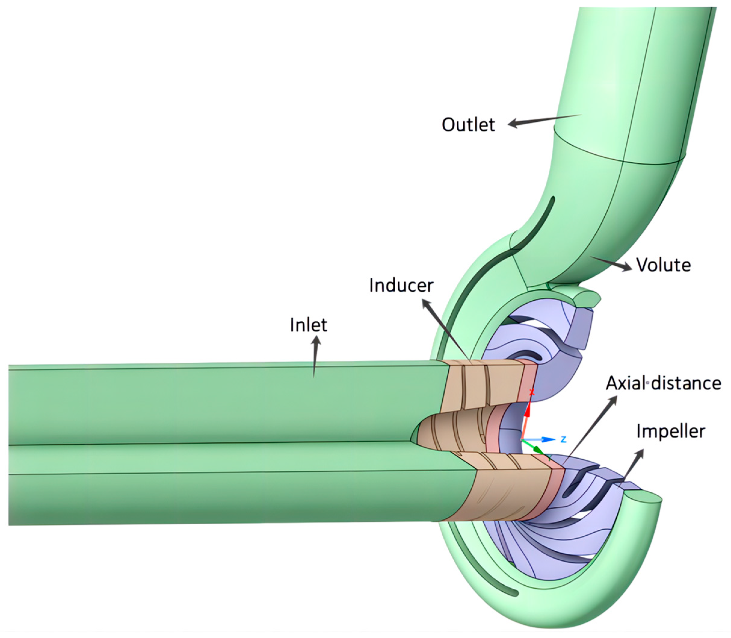
Figure 2.
Calculation domain grid of (a) inducer, (b) volute.

Figure 3.
Grid-independent.

Figure 4.
Fire pump test bench.

Figure 5.
Experimental-simulation performance curves.

Figure 6.
The relationship of duckling and pump.

Figure 7.
The drag reduction coefficients of inducer and impeller at different axial distances.

Figure 8.
The distance between inducer and impeller [18].
Figure 8.
The distance between inducer and impeller [18].

Figure 9.
Impeller performance for some K values.

Figure 10.
Velocity vector.

Figure 11.
Tangential velocity distribution of the trailing inducer for some K values.

Figure 12.
Distribution of kinetic energy for some K values.

Figure 13.
Velocity triangle of impeller inlet.

Figure 14.
Absolute flow angle at impeller inlet for some K values.

Figure 15.
Percentage diagram of entropy production of overflowing components for some K values.

Figure 16.
Absolute value of entropy production of axial distance–impeller for some K values.

Figure 17.
Entropy production distribution from impeller inlet to outlet (a, b, c correspond to the front, middle and rear regions of the impeller).
Figure 17.
Entropy production distribution from impeller inlet to outlet (a, b, c correspond to the front, middle and rear regions of the impeller).

Figure 18.
Impeller inlet pressure distribution (streamwise = 0).

Figure 19.
Expanded flow surface diagram of inducer–axial distance– impeller velocity (the first row of blades is inducer, and the second row is impeller, ①②③④⑤⑥ is the vortex generating region).
Figure 19.
Expanded flow surface diagram of inducer–axial distance– impeller velocity (the first row of blades is inducer, and the second row is impeller, ①②③④⑤⑥ is the vortex generating region).

Figure 20.
Turbulent energy cloud map.

Figure 21.
Impeller-outlet velocity flow plane expanded diagram (the first row of blades is impeller, and the second row is outlet, ⑦⑧⑨ is the region of static and dynamic interference).
Figure 21.
Impeller-outlet velocity flow plane expanded diagram (the first row of blades is impeller, and the second row is outlet, ⑦⑧⑨ is the region of static and dynamic interference).

Figure 22.
Entropy production distribution of the pressure surface–suction surface of the impeller (the first row is the pressure surface of the blade, and the second row is the suction surface of the blade).
Figure 22.
Entropy production distribution of the pressure surface–suction surface of the impeller (the first row is the pressure surface of the blade, and the second row is the suction surface of the blade).

Disclaimer/Publisher’s Note: The statements, opinions and data contained in all publications are solely those of the individual author(s) and contributor(s) and not of MDPI and/or the editor(s). MDPI and/or the editor(s) disclaim responsibility for any injury to people or property resulting from any ideas, methods, instructions or products referred to in the content. |
© 2024 by the authors. Licensee MDPI, Basel, Switzerland. This article is an open access article distributed under the terms and conditions of the Creative Commons Attribution (CC BY) license (https://creativecommons.org/licenses/by/4.0/).
Share and Cite
MDPI and ACS Style
Yang, Z.; Cao, P.; Zhang, J.; Gao, S.; Song, X.; Zhu, R. Research on Energy Loss of Optimization of Inducer–Impeller Axial Fit Dimensions Based on Wave-Piercing Theory. Water 2024, 16, 1385. https://doi.org/10.3390/w16101385
AMA Style
Yang Z, Cao P, Zhang J, Gao S, Song X, Zhu R. Research on Energy Loss of Optimization of Inducer–Impeller Axial Fit Dimensions Based on Wave-Piercing Theory. Water. 2024; 16(10):1385. https://doi.org/10.3390/w16101385
Chicago/Turabian StyleYang, Zhiqin, Puyu Cao, Jinfeng Zhang, Shuyu Gao, Xinyan Song, and Rui Zhu. 2024. "Research on Energy Loss of Optimization of Inducer–Impeller Axial Fit Dimensions Based on Wave-Piercing Theory" Water 16, no. 10: 1385. https://doi.org/10.3390/w16101385
Note that from the first issue of 2016, this journal uses article numbers instead of page numbers. See further details here.