
Differential Analysis of Carbon Emissions between Growing and Shrinking Cities: A Case of Three Northeastern Provinces in China


School of Architecture, Tianjin University, Tianjin 300110, China
*
Author to whom correspondence should be addressed.
Land 2024, 13(5), 648; https://doi.org/10.3390/land13050648
Submission received: 20 March 2024
/
Revised: 5 May 2024
/
Accepted: 8 May 2024
/
Published: 10 May 2024
(This article belongs to the Topic Low Carbon Economy and Sustainable Development)
Abstract
:Carbon emission issues are becoming increasingly severe, and the carbon emissions in shrinking cities, primarily characterized by population loss, are often overlooked and insufficiently studied. This paper focuses on the carbon emissions from county-level administrative units in China’s three northeastern provinces from 2001 to 2017. The study scientifically identified shrinking cities and measured the differences in carbon emission characteristics between growing and shrinking cities using the Theil index. Ultimately, the paper constructs a panel spatial econometric model to analyze the factors influencing them and explore their spatial effects. (1) The total carbon emissions in the Three Northeastern Provinces exhibited an inverted U-shaped trend, increasing from 734.21 million tons in 2001 to 1731.73 million tons in 2017, with the Mann–Kendall trend test showing a significant increase; spatially, this manifests as a significant positive spatial autocorrelation. (2) The region has 138 shrinking cities, accounting for over 50%; regarding carbon emission characteristics, the Theil index has consistently remained above 0.18, indicating significant differences between the carbon emissions of growing and shrinking cities. (3) The panel spatial econometric model results show that the influencing factors of carbon emissions in shrinking cities have unique directions, intensities, and spatial effects. In shrinking cities, aside from localized GDP effects and per-capita GDP acting as a suppressant, the population size has a pronounced inhibitory effect on local and surrounding carbon emissions. The analysis reveals significant differences in the carbon emission patterns and mechanisms between growing and shrinking cities; based on these results, the paper proposes differentiated carbon control strategies.
1. Introduction
Since the Industrial Revolution, human production and life activities have produced vast amounts of carbon emissions, which have had profound negative impacts on the global climate [1]. As the largest developing country globally, China’s carbon emissions have increased annually, making it the world’s largest carbon emitter [2]. In response to this challenge, Chinese President Xi Jinping announced at the 75th United Nations General Assembly in 2020 China’s ambitious goal of reaching a carbon peak by 2030 and achieving carbon neutrality by 2060. This goal is being progressively broken down and implemented across various administrative levels in China, including county-level administrative units.
Regarding total carbon emissions, developed countries generally exhibit higher levels [3]. However, the study by Liu et al. [4] noted a downward trend in Japan’s carbon emissions following the COVID-19 pandemic, contrasting sharply with the situation in Europe and America. This discrepancy highlights variations within developed countries themselves [5]. In developing countries, carbon emission characteristics also vary, as evidenced in the empirical study by Zhang X P et al. [6], which showed that only some developing countries follow the Kuznets environmental curve. Consequently, there are evident differences in carbon emissions among countries or regions at different stages or types [7]. Moreover, research into the factors affecting carbon emissions has garnered considerable scholarly interest. Economic growth, urbanization, and population expansion are widely believed to exacerbate energy demand, thereby increasing carbon emissions [8,9]. For instance, based on data analysis from over 130 countries, York et al. [10] found that urbanization significantly boosts carbon emissions. Chen et al. [11] noted that population agglomeration significantly drives an increase in carbon emissions. Additionally, some scholars hold opposing views [12,13]. The diversity of these research findings has further piqued the academic community’s interest [14,15].
The diversity of carbon emission studies highlights the need for in-depth research on specific areas, such as shrinking cities. Since the 1950s, there has been a worldwide trend of shrinking cities, mainly defined by decreasing populations [16,17]. Shrinking cities often face economic declines, demographic imbalances, and reduced levels of public services [18], which hinder urban development and significantly impact carbon emissions [19]. Schilling J et al. [20] observed that population declines might result in decreased energy use and lower carbon emissions, with shrinking cities benefiting from land reallocation and industrial shifts. However, a reduced population can lead to a looser urban structure and lower efficiency, which are detrimental to environmental protection [21]. Additionally, shrinking cities face declining demand, reducing supply capacity and causing inefficiency in public services like transit, pipelines, and central heating, thereby increasing household carbon emissions [22]. Thus, the relationship between shrinking cities and carbon emissions remains unclear. To explore this issue, a few scholars have attempted to conduct studies by comparing growing and shrinking cities. Xiao HJ et al. [23] concluded that rapidly shrinking cities have the lowest carbon emissions after comprehensively comparing the characteristics of carbon emissions between growing and shrinking cities. An empirical analysis by Tong XH et al. [19] indicates that the carbon emissions of rapidly shrinking cities follow a “U-shaped” curve. However, their studies, along with those of Zeng TY et al. [24], focused too broadly on prefecture-level cities, which do not accurately reflect the actual characteristics of carbon emissions or the implementation of reduction measures. Therefore, there is room for a further empirical assessment of carbon emissions in growing and shrinking cities.
There is a notable scarcity of literature addressing the typical and specific features of carbon emissions in shrinking cities within existing studies. Although existing research has explored carbon emissions between growing and shrinking cities, it is primarily based on broad regional data. It requires detailed analysis, making it easier to implement specific reduction measures. Additionally, few studies have scientifically validated and effectively quantified the differences and extents of carbon emissions between growing and shrinking cities. Crucially, despite the increasing number of studies focusing on carbon emissions in growing and shrinking cities, few have addressed the spatial impacts of these emissions.
To compensate for the existing research deficiencies, this study thoroughly investigated the extent of differences and the characteristics of influencing factors of carbon emissions between growing and shrinking cities. The innovation of this paper manifests in three aspects: Firstly, the paper focuses on the detailed scale of county-level administrative units for carbon emission analysis. The paper uses descriptive statistics and the Mann–Kendall method for a long-term trend analysis of emissions in China’s three northeastern provinces. Secondly, this paper accurately reveals the degree and characteristics of carbon emission differences between growing and shrinking cities by employing quantitative methods such as inter-group differences and the Theil index. Lastly, the paper uses panel spatial econometric models to differentiate the factors influencing carbon emissions in growing and shrinking cities, employing the spatial Durbin model to measure the spatial effects of these factors. This paper proposes differentiated carbon reduction strategies for growing and shrinking cities based on its findings.
2. Materials and Methods
2.1. Scope and Duration of the Study
This study selected the three northeastern provinces of China, where shrinking cities are relatively common [23], as its research area. This region includes the Heilongjiang, Jilin, and Liaoning provinces (Figure 1). Referencing the administrative divisions listed by the Ministry of Civil Affairs of the People’s Republic of China and considering the data distribution characteristics, the study selected 272 cities (county-level administrative units) to analyze the spatiotemporal evolution characteristics of urban carbon emissions. To ensure the accuracy and continuity of the research, 206 of these units were retained to explore differentiated influencing factors.
Regarding the timeline, this research considered crucial junctures such as the 2003 policy to revitalize the northeast’s old industrial bases and the 2016 initiation of a new revitalization strategy for the region. Given the availability of carbon emission data, the study period was set from 2001 to 2017.
2.2. Research Methods and Empirical Models
2.2.1. Mann–Kendall Trend Analysis
Mann–Kendall trend analysis is a non-parametric test method primarily advantageous due to its independence from specific data distributions and its high resistance to missing and outlier values. This method is suitable for trend testing in long-time series data, and it is often used with the Theil–Sen estimator. In conducting the Mann–Kendall test, the null hypothesis posits that the data sequence is random, with no significant trend. Subsequently, statistical measures such as S and the sign function (sgn) are constructed to conduct hypothesis testing, with the specific formulas as follows:
In the above equation, S represents the test statistic, sgn is the sign function, n is the number of data points in the series, and xj and xi are the attributes of the j-th and i-th elements. Subsequent trend analysis utilizes the Z statistic and Var formula as follows:
The meanings of the variables are the same as those in Formula (1). From this, one can determine the confidence intervals for the absolute value of Z based on the confidence level, thereby concluding whether there is a significant change.
2.2.2. Difference Identification Methods
This study utilized the Stata command ttable3, developed by Professor Lian Yujun (see: http://www.lianxh.cn), to test for significant differences in the mean or median total carbon emissions between growing and shrinking cities. The command primarily employs the T-test to compare differences in means or medians, effectively assessing the statistical significance of differences between groups.
Concurrently, this study employs the Theil index as the primary method for quantifying group differences. As a particular form of the generalized entropy index, the Theil index was first introduced by Theil and Henri [25], and it is extensively used to measure inequality among individuals or regions. In the context of this paper, the overall differences can be decomposed into intergroup and intragroup disparities within growing and shrinking cities. A more considerable index value indicates a more significant regional disparity. The specific formula is as follows:
In this formula, N represents the number of groups, yi denotes the proportion of the i-th group’s corresponding indicator to the entire population, and pi represents the proportion of the i-th group’s weighted index to the total.
2.2.3. Analysis Method for Influencing Factors
This research incorporated a range of methods to analyze factors influencing carbon emissions, selecting the best regression model based on comparison across multiple models, as shown in Table 1.
According to Table 1 above, the panel spatial econometric model is undoubtedly the best solution for analyzing carbon emissions at the county level for the following reasons: Carbon dioxide, as the primary carrier of carbon emissions, has strong regional diffusion and easily affects neighboring areas. Furthermore, spatial econometric models can adequately handle the spatial autocorrelation characteristics of carbon emissions and scientifically measure relationships between cities. Moreover, panel data have a rich structure that can appropriately analyze phenomena’s dynamic changes and causal relationships. Therefore, this paper’s analysis uses the panel form of spatial econometric models—panel spatial econometric models—and it uses the results from ordinary panel regression models as a comparative baseline.
This study employed ordinary panel regression models and panel spatial econometric models that consider nested spatial effects to analyze influencing factors.
Commonly used panel regression models include mixed, random, and fixed-effects regression. Model selection can be determined through hypothesis testing, such as the Hausman test, the robust Hausman test accounting for heteroskedasticity, or information criteria like the Akaike Information Criterion (AIC) and the Schwartz Criterion. This paper provides an example by explaining the two-way fixed-effects model using the following formula:
In this equation, yit represents the dependent variable, xit is the explanatory variable, εit signifies the error term, β is the coefficient to be estimated, primarily indicating the marginal impact of x on y, αi represents individual effects, and λit signifies time effects.
In studying spatial units as samples, the spatial effects between the models cannot be disregarded [37]. This aligns with the first law of geography, as Tobler [38] articulated, which states, “Everything is related to everything else, but near things are more related to each other.” The spatial panel econometric model effectively leverages the advantages of panel data and incorporates spatial effects into the model framework, providing a robust tool for analyzing spatial phenomena. Furthermore, it includes spatial lagged dependent variables, error terms, or explanatory variables, thus accounting for spatial dependence. The spatial relationships are defined using a spatial weight matrix, enhancing the model’s versatility and practicality. The most commonly used model is the spatial Durbin model. In this paper, the spatial implication of the spatial Durbin model is that local carbon emissions are influenced not only by local factors but also by neighboring regions’ carbon emissions and other factors. This paper primarily focuses on elucidating the spatial Durbin model (SDM) as follows:
Furthermore, the model can be expressed in vector form:
Here, εt∽N(0,δ2εIn); a = [a1, a2, …, an]; ln is a column vector of dimension (n × 1), with each element being 1; and the other symbols are explained as follows:
The parameters have the same interpretation as those in the panel regression model, with ρ representing the spatial regression coefficient and W denoting the spatial weight matrix. The spatial relationships are defined using wij, indicating the spatial weight relationship between individuals i and j. The abovementioned model can be transformed into a spatial lag model (SLM) or spatial error model (SEM) based on parameter variations.
The spatial lag model (SLM) includes the influence of local emissions on adjacent areas’ emissions within the model, known as spatial spillover effects [39], and it is expressed as follows:
In the formula, the variables are the same as those in the previous formula, X-X, where μi denotes the individual fixed effects.
In prevalent spatial regression models, there is potential for spatial autocorrelation in the independent error terms, leading to the development of the SEM, presented as follows [37]:
Generally, the best panel spatial econometric model selection can be determined using the Lagrange Multiplier test or evaluated through post-regression information criteria [40].
2.3. Construction of Influencing Factors
The data used in this study were categorized into three types: total carbon emissions data, population data to identify shrinking cities, and socioeconomic data to analyze factors affecting carbon emissions. The carbon emission data came from the Carbon Emission Accounts and Datasets (CEADs) [41], which provided county-level carbon emissions data for China from 1997 to 2017 (https://www.ceads.net/data/county/; accessed on 29 January 2024). The CEADs have been harmonized using Particle Swarm Optimization-Back Propagation (PSO-BP) algorithms applied to DMSP/OLS and NPP/VIIRS satellite images to estimate the carbon emissions of county-level administrative units in China, thereby filling gaps in research at this level. Furthermore, population data were obtained from the WorldPop database (https://hub.worldpop.org). These data, primarily based on population censuses, nighttime lights, terrain, and proximity to critical elements, are spatialized using random forest algorithms, offering a better spatiotemporal resolution than other population datasets [42]. Lastly, data on influencing factors for carbon emissions primarily came from the “China County Statistical Yearbook” (2000–2018) published by the National Bureau of Statistics of China (https://www.stats.gov.cn/); additional land use data were from the China Land Cover Dataset database [43], noted for its high spatiotemporal consistency and superior accuracy.
The data were normalized to a standard normal distribution to mitigate the effects of scale and magnitude differences.
For the construction of influencing factors for carbon emissions, the impacts of economic development, population size, industrial structure, and policy regulations within county-level administrative units were considered, with relevant data from Table 2 analyzed.
China’s rapid urbanization has been driven by heavy industries such as cement, steel, and power generation [44]. However, constrained by relatively inefficient production processes and energy utilization, industries like cement exhibit higher carbon emission intensities than the global average [45], leading to significant carbon emissions. Nonetheless, it is worth noting that optimizing the structure of urbanization can enhance efficiency and reduce carbon emissions [46]. Furthermore, during this process, factors such as general public budget revenue and expenditure play pivotal roles in evaluating China’s fiscal capacity, particularly in infrastructure development and ensuring citizens’ well-being [47,48]. Thus, construction land area, general public budget revenue, and expenditure were selected as factors influencing carbon emissions for analysis.
The expansion of an economic scale is achieved through the consumption of resources, including energy. In China, the growth of carbon emissions is closely tied to the rapid development of the economic scale, a scenario unlikely to be avoided in the short term [49]. As a responsible global actor, China must optimize its economic structure to achieve high-quality development [50]. This necessitates a shift from resource-intensive industries towards low-carbon industries to increase the proportion of clean energy and improve carbon emission efficiency, ultimately achieving emission reduction goals. However, more than just transitioning the secondary sector to high-end services and high-tech industries is not advisable, as this approach may inadvertently become a new source of carbon emissions [51,52]. Moreover, considering the significance of the Environmental Kuznets Curve hypothesis on the inverted “U” shape of per-capita income, this study comprehensively selected factors including the gross domestic product (GDP), output value of secondary industries, output value of tertiary industries, and per-capita GDP as influencing factors.
Extensive interactions exist between population and carbon emissions, and the relationship is often generated indirectly through consumption, production, and trade pathways. Previous research has confirmed that, under constant conditions, changes in the population scale influence energy demand, the construction land scale, and the consumption scale, subsequently affecting carbon emissions [53]. The relationship between the population scale and carbon emissions is not a simple, linear one; it is influenced by regional characteristics, urban types, and even consumption habits [54]. Therefore, this study selected the population scale as one of the factors for subsequent analysis.
2.4. Principles and Methods for Identifying Shrinking Cities
Shrinking cities are characterized by population losses, economic declines, social unrest, or vacant land [55]. Although there is still a debate over the specific methods for identifying shrinking cities, a decline in the population size is commonly accepted as a core characteristic [56]. For instance, considering the low population of small towns in Europe and America, the Shrinking Cities International Research Network defines cities of over 10,000 that have been experiencing a population decline and a structural economic crisis for over two years as shrinking cities [57]. Wirchmann T [58] considers two consecutive years of population decline to indicate a shrinking city. However, some scholars regard cities with population growth rates below the average as shrinking cities [59].
In summary, to enhance the stability and continuity of identification, this study considered the number of years of population losses and the extent of cumulative declines as critical factors. Drawing on related studies [60], this paper first calculated the cumulative count of population decreases (Count, c, measured in pieces) and the rate of population size changes (Rate, r, in percentage) for each county-level administrative unit. It then established classification thresholds based on data trends and constructed a matrix to categorize cities into growing and shrinking groups (Table 3).
3. Results
3.1. Spatiotemporal Evolution of Carbon Emissions
The initial step involved describing and analyzing the temporal variation characteristics of carbon emissions in the three northeastern provinces, utilizing mathematical statistics and the MK trend test method (Table 4).
A stacked bar chart was plotted to analyze the temporal development characteristics of carbon emissions in the three northeastern provinces (Figure 2). As shown in Figure 2, the total carbon emissions in the three northeastern provinces increased from 734.21 million tons in 2001 to 1731.73 million tons in 2017 at an average annual growth rate of 5.51%. In terms of the growth rate, it shows a fluctuating decline trend. Before 2006, the growth rate fluctuated but remained above 10%. After 2007, the growth rate briefly accelerated and rapidly declined, maintaining positive growth of about 5%. After 2015, it directly dipped to around −5%. Although progress has fluctuated, total carbon emissions gradually increased and stabilized to approximately 1750 million tons after 2015. Next, the paper used the MK trend test method to verify the growth trends in carbon emissions for the entire region and each province (Table 4). As shown in Table 4, the total carbon emissions and carbon emissions from each province in the study area exhibited a stable growth trend at a 95% confidence level, and the differences in Sen’s slope values among provinces indicated regional disparities.
Combining the analysis from Figure 2 and the above information, we observed that the carbon emissions in the region followed an “M-shaped” curve. There was a period of rapid growth from 2001 to 2006, followed by a slowdown influenced by the “Revitalizing the Old Industrial Bases in Northeast China” policy and fluctuations in the domestic and international economic situation. After 2010, the carbon emissions peaked at around 1830.11 million tons due to population outflows and technological improvements. Subsequently, emissions transitioned from growth to decline, and they have gradually stabilized.
When comparing the provinces, Liaoning Province, known for its abundant resources and energy industries, contributes to nearly half of the region’s total carbon emissions, partly explaining the relatively lower proportion of shrinking cities in the province. Both the Heilongjiang and Jilin provinces have a roughly equal share of carbon emissions, each accounting for about one-fourth of the total. The stability of these proportions across the three provinces indicates a steady development in Northeast China. It suggests that there has yet to be a clear trend in localized technological progress or overall expansion in carbon emissions.
Then, Moran’s I index was used to measure the spatial evolution characteristics of carbon emissions in the three northeastern provinces.
As shown in Figure 3, Moran’s I index, which measures the overall spatial autocorrelation, was significant at a 1% confidence level and consistently stayed above 0.30. Moran’s I index indicates that the county-level carbon emissions in the region had a positive spatial dependence over the years. Additionally, Moran’s I index shows three stages of evolution: a stable fluctuation, a linear increase, and a sharp decline, with the main turning point occurring around 2011–2012.
To explore the clustering relationship of carbon emissions in local areas, we conducted an analysis of local indicators of spatial association based on the cross-sectional data in 2017. The results in Figure 4 reveal robust local spatial autocorrelation patterns in the Northeast China region. The clustering is primarily divided at the border between the Heilongjiang and Jilin provinces. The northern part of Heilongjiang Province exhibits stable and low–low clustering, while the “Changchun-Shenyang-Dalian” urban axis in the southern part shows stable and high–high clustering characteristics. Over the years, the low–low clustering area in the north consisted of three main spatial clusters: Qiqihar, Yichun, and Mudanjiang. The high–high clustering of the “spatial club” phenomenon was observed in cities like Changchun, Shenyang, Dalian, and Panjin.
3.2. Results of Identification of Shrinking Cities
This study employed a Two-Step Identification Approach to classify cities within the region, aiming to identify different types of shrinking cities and understand their spatial and temporal distribution patterns. Firstly, based on provinces, a bidirectional table of city types (Table 5) was constructed to identify the distribution of different types of cities.
Table 5 shows that even with relatively strict identification criteria, we identified 138 shrinking cities within the region, accounting for over 50%. Jilin Province has the highest proportion of shrinking cities, reaching 56.9% among the provinces. Liaoning Province has slightly more growing cities than shrinking ones, which is better. Heilongjiang Province has the second-highest proportion of shrinking cities, exactly reaching the 50% mark, making it the province with the highest number of shrinking cities among the three. The amount indicates that shrinking cities have essentially taken up a significant portion of the three northeastern provinces, becoming widespread.
The spatial distribution maps of shrinking and growing cities are generated to comprehensively express the spatial distribution characteristics of shrinking cities (Figure 5). As shown in Figure 5, cities of different types tend to cluster together in specific spatial patterns. Growing cities are primarily concentrated around the central cities and their surrounding areas. There are three main spatial clusters: the Harbin urban agglomeration, the cluster of Changchun and its surrounding cities, and the crowd of Dalian and its surrounding cities. In contrast, shrinking cities were divided into three regions: the northern border area, the central region with resource depletion, and the southwestern province. This spatial distribution pattern highlights the significant role of major or large cities in driving the development of their surrounding cities. It provides strong evidence supporting China’s urban agglomeration or metropolitan development strategies.
This paper used ttable3 and related commands in Stata to conduct between-group difference tests in order to assess the difference in carbon emissions between growing and shrinking cities.
The intergroup mean and median differences between different types of cities were measured using the t-table command, as shown in Table 6. The table above shows that the mean and median tests for carbon emissions between growing and shrinking cities are significant at the 1% confidence level.
To further test the difference in carbon emissions between shrinking and growing cities, the Theil index was used to measure the degree of differentiation between the types (Figure 6). As shown in Figure 6, the Theil index has consistently remained above 0.18, with a mean of 0.19 and a peak of 0.210 in 2011. The analysis of Theil coefficient results reveals significant intergroup differences in carbon emissions between different types of cities, and these differences have increased over the years. These findings confirm the robustness of intergroup differences. Over time, the development of the Theil coefficient can be divided into three stages: 2001–2007 as the “V-shaped” development period, with the coefficient declining from 0.19 in 2001 to a minimum in 2004, followed by a steady rise to around 0.21 in 2011. With the previous Moran index analysis, it can be inferred that significant changes occurred in the spatial characteristics and intergroup relationships of carbon emissions in the region during 2011–2012, warranting further exploration.
The contributions of the two types of cities to the overall differences have shown an alternating upward trend. The contribution of growing cities started below 50% in 2001, fluctuated and slowly rose to 47% in 2010, and then experienced a rapid surge, followed by a tendency to decline, and finally, a steady increase, stabilizing at a contribution rate of 52%. On the contrary, the contribution of shrinking cities was the opposite.
The above analysis methods from different perspectives confirm the differences in carbon emissions between different types of cities. Similarly, the differences were attributed to structural characteristics such as different stages of urban development, the economic scale, the total population, industrial structures, and government expenditure preferences. Do the factors influencing carbon emissions in shrinking cities differ from those in growing cities? Are there variations in low-carbon planning strategies or starting points? These aspects warranted further investigation to explore the heterogeneity caused by urban type differences. To achieve this, sample segmentation was employed to examine the differentiated characteristics and influencing factors of carbon emissions in different types of cities.
3.3. Panel Analysis of Influencing Factors of Growing and Shrinking Cities
Given the substantial differences in carbon emissions between growing and shrinking cities in the three northeastern provinces, and considering the spatiotemporal characteristics and current status of various city types, this study adopted a classification-oriented approach. Using panel regression and panel spatial econometric models, it sought to analyze the differentiated characteristics of factors influencing carbon emissions among three groups of samples: the entirety of the three northeastern provinces, shrinking cities, and growing cities. The objective was to explore each city type’s distinctiveness of influencing factors and elucidate their unique impact mechanisms.
The study selected 206 complete and coherent cities for regression analysis. Based on theoretical deductions, the variables underwent tests for correlation, white noise, and the short panel unit root to verify the model’s stability, and a collinearity test was conducted. The test results demonstrate that all the sample groups exhibited stable data without heteroscedasticity and showed a significant correlation between the explanatory and explained variables, validating the use of panel regression models. Subsequently, the xttest0 and xtoverid commands were employed to test the suitability of random and mixed regression, as well as random and fixed effects, and to examine time and the individual impact. The results of these tests indicated that the individual–time two-way fixed effects model was more appropriate for the analysis in this study.
This study employed the Stata 17 software to conduct bi-directional fixed effects regression analysis on three groups of samples, including the overall cities (1), growing cities (2), and shrinking cities (3), based on the inverse distance-squared spatial weight matrix. It obtained the regression results of models (1), (2), and (3) (Table 7).
In general, there were significant differences in the significance, direction, and strength of variables in models (1), (2), and (3). Only GDP, SSI, and STI exhibited significance across all sample groups.
Upon reviewing the regression results for GDP and GDPPC, it was observed that GDP consistently exerted a significant, favorable influence on carbon emissions across all the models. Conversely, GDPPC showed a promoting effect in model (2) and an inhibiting effect in model (3). When considering the Environmental Kuznets Curve and the relatively diminished economic scale of shrinking cities, it is evident that GDP, as a critical indicator of regional economic development, still presents varying degrees of a promoting effect on carbon emissions in the region. However, the level of regional development based on GDPPC remains on the left side of the “turning point,” especially pronounced for shrinking cities (an elasticity coefficient of 0.27, more significant than the overall and growing cities). Moreover, the direction of GDPPC’s effect significantly diverged from the results aligning with the Environmental Kuznets Curve, which assumes an inverse “U” shape for per-capita income. Hence, it is necessary to refine city types based on regional conditions, economic quantities, and structured characteristics. The abovementioned result provided further insights into cities’ carbon emission compositions at different development levels.
The significant effect of PS was only observed in model (3), and it appeared as an inhibiting factor. However, despite being characterized by population shrinkage and economic contraction, shrinking cities exhibited a rising trend in carbon emissions with continuous population losses. This conclusion aligns with similar findings by some scholars [61]. Considering China’s relatively low carbon emission efficiency, phenomena such as population outflows and economic contraction may further reduce energy efficiency, increasing total carbon emissions to some extent.
GPBR and GPBE only exhibited a promoting effect in model (3), and the strength of their effects was relatively weak. The regression results suggest that the direct impact of these variables on carbon emissions is insignificant.
CLA, which supports the main productive and living activities of the region, demonstrated a significant promoting effect in models (1) and (2) but not in model (3). This disparity may be attributed to expanding land use in growing and shrinking cities and the mixed usage in gradually “hollowed-out” developed areas, diluting CLA’s significant influence on carbon emissions.
Well-acknowledged carbon emission heavyweights SSI and STI consistently exhibited a significant inhibiting effect across all models. The three northeastern provinces, renowned as “old industrial bases,” have faced internal and external structural and systemic issues, such as resource depletion, economic transitions, and financial crises. These factors have contributed to the declining development dynamics of output value of secondary industries, resulting in insufficient vitality and enduring significant impacts. Despite undergoing “growing pains” through scale reductions, these provinces have gradually shifted towards an inhibitory effect. On the other hand, the optimization and enhancement of output value of tertiary industries often entail “high added value,” “high technology,” and “green” attributes, enabling productivity enhancements and energy optimization and, consequently, effectively reducing carbon emissions [62].
A reference to the relevant literature indicates that FAI can lead to prolonged and substantial carbon emissions under the amplification of multiplier effects. Given the persistently high growth levels of fixed asset investments, including construction projects and significant infrastructure, within the three northeastern provinces during the study period, combined with the alignment of FAI with economic development and the lag effect on economic stimulus, FAI demonstrated a significant promoting effect in models (1) and (2).
3.4. Spatial Panel Analysis of Influencing Factors for Growing and Shrinking Cities
Based on the significant positive spatial autocorrelation features of carbon emissions indicated in the previous Moran’s I index, the panel spatial econometric model with spatial effects was employed for analysis.
The selection of the model form is essential and fundamental in applying spatial econometric models. In terms of model selection, a comprehensive analysis was conducted using the spatial error model (SEM), spatial lag model (SLM), and spatial Durbin model (SDM). Subsequently, the Wald-test and lr-test were performed to determine whether the SDM model needed to be degenerated. The results indicated that the SDM model was the most suitable for analyzing all samples. Therefore, regression analysis was conducted, and the estimation results are shown in Table 8, where “W*” represents the lag term.
By comparing Table 7 and Table 8, it can be observed that the information criteria of the panel spatial Durbin model were significantly better than those of other models for the same sample. Although there were some differences in the direction and strength of regression coefficients, they were consistent, indicating the stability and specialization of the panel spatial Durbin model in capturing spatial characteristics. The spatial interaction coefficient rho was significantly positive, suggesting that an increase in local carbon emissions led to a rise in neighboring areas, indicating a positive spatial relationship.
Since the SDM suffers from the limitation of difficult-to-interpret regression coefficients and the inability to capture nonlinear features, we employed LeSage and Pace’s method [63] to decompose the effects of models (4), (5), and (6) into direct effects (DEs), which represent effects on the local region, and indirect effects (IEs), which represent effects on neighboring areas. The results are presented in Table 9.
The direct and indirect effects of GDP in models (4) and (5) were consistent with the results of the previous models, showing significant promoting effects. The regression result indicates that the increase in the GDP in both the overall and growing cities significantly stimulated carbon emissions in the local region and neighboring areas. The lack of significance for the indirect effect of GDP in model (6) suggests that the shrinking cities, characterized by a relatively reduced economic scale, have partially lost their influence on neighboring cities’ carbon emissions. The inhibiting direct and indirect effects of GDPPC in model (6) suggest that the development stage of shrinking cities has crossed the turning point of the Environmental Kuznets Curve. However, in reality, the shrinking of the development scale and the regression of the level led to a leftward shift of the horizontal axis, thus reversing the impact of per-capita income on carbon emissions.
The direct and indirect effects of PS in models (4) and (5) were significant in promoting and inhibiting carbon emissions, respectively, with the effect strength in model (5) notably stronger than in model (4). The regression result indicates that the continuous accumulation of a population in growing cities exacerbates carbon emissions within the region. In model (6), both the direct and indirect effects of PS exhibited inhibiting characteristics, which align with the results in Section 3.2. This result further emphasizes how the dwindling of a shrinking city due to a population outflow reverses the conventional impact pattern, causing an increase in per-capita carbon emissions’ intensity and transforming the stimulus to inhibition for the shrinking city itself and its surrounding areas.
The effects of GPBR and GPBE are intriguing. The direct effects of GPBR were all promoting, with the indirect effect being significant only in model (5) as a low-level promotion. In contrast, the significance of GPBE was precisely the opposite: its direct effects were relatively weak, with only low-level advertising in model (5), and insignificant in the other models. However, its indirect effects were consistently significant and inhibiting, indicating a negative spatial spillover effect, leading to a restraint on carbon emissions in neighboring areas. This finding suggests that growing cities exhibit important agglomeration and scale effects due to their robust economic and social vitality and noticeable amplification effects on expenditures and income. It also highlights the scientific and necessary nature of classification analysis, which helps discern individual sample characteristics and avoids concealing results due to overall analysis.
CLA’s direct and indirect effects in each model exhibit significant promotion and inhibition, respectively. Expanding the construction land scale implies a demand for building materials and fossil fuels and the support of primary production and daily activities, promoting local carbon emissions during construction and usage. The enlargement of local construction land also strengthens the “Matthew Effect” to some extent, thereby displaying the inhibition of neighboring carbon emissions. Moreover, the effect intensity indicates that developmental and prosperous growing cities with active factors show the most promote impact on CLA.
SSI exhibited significant inhibitory direct and indirect effects in each model. Under the pressure of external favorable conditions such as the rise of the “old industrial base” in the three northeastern provinces, along with internal factors like resource depletion and population losses, these regions actively transitioned and substituted industries, developed circular economies, and implemented approaches “replacing older industries with newer ones,” effectively enhancing the industrial carbon emission efficiency, leading to an inevitable reduction in total emissions. Simultaneously, the surrounding areas benefited from a technology transfer and experience dissemination, i.e., the “free ride” effect, decreasing carbon emissions.
STI exhibited significant inhibitory effects across multiple models. This result indicates that, under the combined influence of technological innovation, infrastructure development, and ecological civilization guidance, STI is gradually transitioning and upgrading toward the green tertiary industry. It also exerts a positive spatial driving effect on the STI of neighboring cities. Through synergistic effects with industries in neighboring cities, carbon emission efficiency is improved, facilitating the achievement of regional carbon reduction goals.
On the other hand, FAI continued to exert a strong promoting effect on local carbon emissions, which was particularly evident in the overall growth of cities. Interestingly, this factor’s impact on local carbon emissions was insignificant in model (6), but it inhibited carbon emissions in surrounding areas. FAI is a crucial driver of local economic development in China, demonstrating notable economies of scale. However, the analysis in this study reveals that its marginal effect is not strictly linear and might have a specific threshold value. Only after surpassing this threshold value does the marginal impact of FAI on carbon emissions become apparent. In cities or regions that are relatively backward or experiencing declines, the effect of FAI on carbon emissions remains weak when it fails to break through the bottleneck constraints.
4. Discussions and Conclusions
4.1. Analysis of Differences in Influencing Factors between Growing and Shrinking Cities
In general, shrinking cities are also a normal stage in the cyclical pattern of urban development, representing one of the inevitable phases in urban emergence, growth, prosperity, decline, and transformation. However, under the goals of the carbon peak and carbon neutrality, cities, significantly shrinking cities that have experienced structural crises face more daunting challenges in terms of transformation and emission reduction pressures [64]. Therefore, based on the results of carbon emission evolution differences and panel spatial econometric regression analysis, and in comparison with relevant research, this study attempted to conduct a detailed analysis of the differences in influencing factors between growing and shrinking cities.
The findings of this study further confirm that, in China, the GDP has a strong promoting effect on carbon emissions. A comparison with studies from developed countries like those in Europe and the United States [65] reveals that most cities in China are still in relatively early stages of development, with carbon emissions per unit of GDP exceeding the global average [66]. China still maintains a development model oriented towards economic growth, and the inertia of development, characterized by a high scale and low efficiency, persists. Considering the inhibitory effects of output values of secondary and tertiary industries on carbon emissions observed in this study, we can conclude that, in the research area, especially in shrinking cities (with the smallest absolute regression coefficient), efforts should be directed toward optimizing these industries’ energy efficiency and cleanliness. This phenomenon would further reduce the carbon emissions per unit of GDP and achieve sustainable and healthy development.
For shrinking cities, although the decrease in the population scale inhibits carbon emissions, their development patterns are unhealthy. This result contrasts with findings based on the IPAT equation, but it aligns with the results of Xiao HJ et al. [23]. Why do studies with similar questions yield different conclusions? Possible reasons include: first, interactions between independent variables in the model setup might have obscured the underlying mechanisms; second, the panel spatial econometric model used in this paper incorporated spatial effects, providing a more accurate reflection of the mutual influences between cities. Considering the region’s relatively low per-capita income levels and the prevalent phenomenon of population outflows, a decrease in the population scale might lead to a reduction in carbon emission efficiency. However, under comprehensive effects, it is more likely to result in a reduction in total carbon emissions.
4.2. Optimization Paths for Carbon Emissions in Growing and Shrinking Cities
Based on the above analysis, this paper attempts to propose suggestions to optimize carbon emissions for different types of cities.
Firstly, shrinking cities are prevalent and widely distributed in the three northeastern province region. Differentiated emission reduction policies should address spatial heterogeneity, inter-group differences, and distinct influencing factors between growing and shrinking cities [67]. For shrinking cities, it is essential to leverage the scale and agglomeration effects of the GDP, promoting economic development while aligning with technological trends, accelerating energy transformation, and driving economic advancement towards high-end, green, and intelligent sectors. In terms of population, efforts should be directed toward improving livelihoods, optimizing the employment environment, supplying service-oriented consumption, and attracting people and talent to reverse the trend in the population outflow and the simultaneous increase in carbon intensity. In summary, selecting key areas, focusing efforts, and achieving precise breakthroughs are essential to achieving more with less effort.
In expanding the scope nationwide, considering the differences in developmental stages or types of cities, and facing the dual challenges of steady economic growth and the objectives of the “carbon peak” and “carbon neutrality,” it is crucial to identify the carbon emission characteristics and influencing factors of specific regions or cities. Prioritizing spatial interactions between cities, understanding internal and external effects patterns, actively mitigating and adapting to global or local climate changes, and fostering a new type of urbanization while promoting sustainable, high-quality development is imperative.
Secondly, emphasis should be placed on the spatial effects of various factors. Carbon emissions and their influencing factors demonstrate significant spatial dependency within regions. Thus, establishing low-carbon cities as pilot points could harness their leadership role while driving the simultaneous improvement in surrounding areas. A holistic consideration of adjacent regions is essential, strengthening the synergy, synchronicity, and linkage of policy formulation and strategic implementation. Steadily advancing the development of urban clusters or metropolitan areas will enhance carbon emission efficiency and reduce overall carbon emissions.
In conclusion, given China’s vast territory, pronounced regional disparities, uneven economic development, and asynchronous social progress, cities of different types should align with their unique structural characteristics and clarify their developmental stages and main strengths. Regions with the necessary conditions can focus on developing carbon capture and storage technologies [68]. Moreover, multidimensional approaches encompassing economic decarbonization, green industries, energy efficiency, and low-consumption habitats should be adopted. Focusing on areas with the highest suitability and compatibility for “low-carbon” practices, addressing weaknesses, bolstering strengths, and pursuing context-based and customized “dual-carbon” pathways are crucial. At the same time, comprehensive coordination at the provincial and regional levels is necessary to implement a strategic plan that encompasses the whole country. This approach should pave the way for China’s decarbonization journey by prioritizing regions with the capability to peak emissions first and leveraging the experiences of less advanced areas.
4.3. Research Applicability and Generalizability
This study conducted an in-depth analysis of the differences in carbon emissions among county-level administrative units in China’s three northeastern provinces, particularly quantifying the differences between growing and shrinking cities, thereby revealing characteristics and spatial effects of total carbon emissions. The methods used in this study effectively address issues such as carbon emission development trends, the quantification of differences between groups, and the identification of spatial effects among different types of cities within a region.
Mann–Kendall trend analysis is highly applicable to handling outliers and missing values in environmental data. It is particularly suited for assessing the significance of trends in time-series data. Moreover, this method is particularly effective in analyzing the turning points of industrial carbon emissions [69] and predicting peak regional carbon emissions [70].
The Theil index offers a detailed perspective on analyzing intra-group inequalities, widely applied from differences in carbon emissions in urban residential buildings [71] to variations in emission intensities between industries [72] and comparisons of emission efficiencies between countries [73].
Furthermore, the panel spatial econometric model leverages the dynamic analysis of panel data while providing more accurate causal inferences about the interactions between the spatial and temporal dimensions of carbon emissions [74]. In this paper, the model has also accurately quantified the spatial dependency of urban carbon emissions, aided in explaining the interaction and transmission mechanisms of carbon emissions, and significantly enhanced the model’s explanatory power, thereby supporting the formulation of targeted emission reduction strategies.
In summary, the various methods guided by the research framework of this paper are widely applicable and extensible in the field of carbon emission studies.
4.4. Research Limitations and Prospects
This paper still has certain limitations. Firstly, there needs to be more spatial entity constraints in the scope of such research. This study analyzed the grassroots-level units in China’s county-level administrative divisions. While this research scale contributes to implementing emission reduction measures and control policies, it overlooks the distinction between physical cities and administrative cities, which could potentially introduce research errors [74]. Secondly, the methodology for examining influencing factors must consider city-level classification systems. This empirical study compared differences in regression coefficient significance, direction, and strength between the influencing factors of growing and shrinking cities’ carbon emissions. This method is ordinary and necessary, as many scholars explore similar phenomena using the same approach [75]. However, some scholars argue that comparing the regression differences of sub-sample coefficients solely could lead to bias, and they suggest using tests like the Chow test, a seemingly unrelated regression test, or Fisher’s permutation test to address this issue. However, these tests have limitations in handling cross-product heteroskedasticity, and they do not apply to panel spatial econometric models.
Consequently, future research should distinguish between the differences in the carbon emissions of physical and administrative cities. In selecting a research scope, more detailed regional refinement or the selection of specific cities for in-depth analysis is advisable. Moreover, statistical methods should be employed to verify the differences in grouped regression coefficients using a hypothesis-testing approach based on the panel spatial econometric model. This improvement would further enhance the readability and scientific validity of future studies.
5. Research Conclusions
The Chinese government places significant emphasis on the sustainable development of the northeastern region, introducing a series of strategic policies to support its revitalization. The rise and development of the three northeastern provinces have achieved noticeable progress and stage results. Delving into the evolution and type differences of carbon emissions among cities aids various regions in implementing distinctive “dual-carbon” paths aligned with their city types and actual circumstances. The main conclusions of this study are as follows.
(1) Numerous shrinking cities show a spatially clustered distribution pattern. They are based on the core indicator of population size, and classified urban types within the region; 138 shrinking cities were identified, accounting for over 50% of the total. Their distribution among provinces is balanced, signifying the widespread and typical nature of the shrinkage issue in the region. In contrast, growing cities outside of the shrinking category form spatial clusters centered around Harbin, Changchun, Dalian, and surrounding cities, demonstrating the driving role of large cities in population and economic aspects.
(2) Carbon emissions are steadily increasing, with notable disparities among urban types. In 2017, the overall carbon emissions in the three northeastern provinces reached 1731.73 million tons, a 2.36-fold increase from 2001. The growth trend passes the MK trend test, and the tendency follows a “U-shaped” curve characterized by periods of accelerated growth, deceleration, and a gradual slowdown. Additionally, a significant positive spatial autocorrelation relationship exists. The paper employed the t-table command, confirming substantial differences in carbon emissions’ mean and median values between shrinking cities and growing cities. The Theil coefficient also highlights the practical disparities in carbon emissions between growing and shrinking cities.
(3) The panel spatial Durbin model yielded the best information criteria among the regression models employed in this study. The regression results of this model revealed that the main influencing mechanisms and spatial effects of carbon emissions differ significantly between growing and shrinking cities. Regarding the direct and indirect effects of the spatial Durbin model (SDM), factors such as GDP, CLA, SSI, and STI exhibited similar directional tendencies in both city types but with varying intensities. Furthermore, due to the relatively dwindling population and economic scale of shrinking cities, they tend to move away from the carbon emission peak, suggesting their transition toward a decline. The effect of population size further underscores the “regression” of shrinking cities.
Author Contributions
Conceptualization, Y.S. and W.H.; methodology, Y.S. and W.H.; software, Y.S. and W.H.; data curation, Y.S. and W.H.; writing—original draft preparation, Y.S. and W.H.; writing—review and editing, Y.S. and A.N.; visualization, Y.S. and A.N.; supervision, A.N. and J.Z.; project administration, J.T. and J.Z.; funding acquisition, J.T. and J.Z. All authors have read and agreed to the published version of the manuscript.
Funding
This research was funded by the National Natural Science Foundation of China (Grant No. 52378065).
Data Availability Statement
No new data were created or analyzed in this study. Data sharing is not applicable to this article.
Conflicts of Interest
The authors declare no conflicts of interest.
References
- Bilgen, S. Structure and environmental impact of global energy consumption. Renew. Sustain. Energy Rev. 2014, 38, 890–902. [Google Scholar] [CrossRef]
- Sun, W.; Huang, C. Predictions of carbon emission intensity based on factor analysis and an improved extreme learning machine from the perspective of carbon emission efficiency. J. Clean. Prod. 2022, 338, 130414. [Google Scholar] [CrossRef]
- Xiao, Y.; Ma, D.; Zhang, F.; Zhao, N.; Wang, L.; Guo, Z.; Zhang, J.; An, B.; Xiao, Y. Spatiotemporal differentiation of carbon emission efficiency and influencing factors: From the perspective of 136 countries. Sci. Total. Environ. 2023, 879, 163032. [Google Scholar] [CrossRef] [PubMed]
- Liu, Z.; Deng, Z.; Davis, S.J.; Giron, C.; Ciais, P. Monitoring global carbon emissions in 2021. Nat. Rev. Earth Environ. 2022, 3, 217–219. [Google Scholar] [CrossRef] [PubMed]
- Wu, Y.; Zhu, Q.W.; Zhu, B.Z. Comparisons of decoupling trends of global economic growth and energy consumption between developed and developing countries. Energy Policy 2018, 116, 30–38. [Google Scholar] [CrossRef]
- Zhang, X.P.; Zhang, H.N.; Yuan, J.H. Economic growth, energy consumption, and carbon emission nexus: Fresh evidence from developing countries. Environ. Sci. Pollut. Res. 2019, 26, 26367–26380. [Google Scholar] [CrossRef] [PubMed]
- Liu, C.; Su, Y. Classification of China’s county administrative units based on carbon emissions from energy consumption and economic indicators. Int. J. Global. Warm 2021, 23, 255–273. [Google Scholar] [CrossRef]
- Knapp, T.; Mookerjee, R. Population growth and global CO2 emissions: A secular perspective. Energy Policy 1996, 24, 31–37. [Google Scholar] [CrossRef]
- Dong, K.; Hochman, G.; Zhang, Y.; Sun, R.; Li, H.; Liao, H. CO2 emissions, economic and population growth, and renewable energy: Empirical evidence across regions. Energy Econ. 2018, 75, 180–192. [Google Scholar] [CrossRef]
- York, R.; Rosa, E.A.; Dietz, T. STIRPAT, IPAT and ImPACT: Analytic tools for unpacking the driving forces of environmental impacts. Ecol. Econ. 2003, 46, 351–365. [Google Scholar] [CrossRef]
- Chen, J.; Wang, L.; Li, Y. Research on the impact of multi-dimensional urbanization on China’s carbon emissions under the background of COP21. J. Environ. Manag. 2020, 273, 111123. [Google Scholar] [CrossRef] [PubMed]
- Chikaraishi, M.; Fujiwara, A.; Kaneko, S.; Poumanyvong, P.; Komatsu, S.; Kalugin, A. The moderating effects of urbanization on carbon dioxide emissions: A latent class modeling approach. Technol. Forecast. Soc. 2015, 90, 302–317. [Google Scholar] [CrossRef]
- Kenworthy, J.R.; Laube, F.B. Automobile dependence in cities: An international comparison of urban transport and land use patterns with implications for sustainability. Environ. Impact. Asses. 1996, 16, 279–308. [Google Scholar] [CrossRef]
- Shuai, C.; Shen, L.; Jiao, L.; Wu, Y.; Tan, Y. Identifying key impact factors on carbon emission: Evidences from panel and time-series data of 125 countries from 1990 to 2011. Appl. Energy 2017, 187, 310–325. [Google Scholar] [CrossRef]
- Poumanyvong, P.; Kaneko, S. Does urbanization lead to less energy use and lower CO2 emissions? A cross-country analysis. Ecol. Econ. 2010, 70, 434–444. [Google Scholar] [CrossRef]
- Großmann, K.; Bontje, M.; Haase, A.; Mykhnenko, V. Shrinking cities: Notes for the further research agenda. Cities 2013, 35, 221–225. [Google Scholar] [CrossRef]
- Yang, Y.; Wu, J.G.; Wang, Y.; Huang, Q.X.; He, C.Y. Quantifying spatiotemporal patterns of shrinking cities in urbanizing China: A novel approach based on time-series nighttime light data. Cities 2021, 118, 103346. [Google Scholar] [CrossRef]
- Hartt, M.; Hackworth, J. Shrinking Cities, Shrinking Households, or Both? Int. J. Urban Reg. 2020, 44, 1083–1095. [Google Scholar] [CrossRef]
- Tong, X.; Guo, S.; Haiyan, D.; Duan, Z.; Gao, C.; Chen, W. Carbon-Emission Characteristics and Influencing Factors in Growing and Shrinking Cities: Evidence from 280 Chinese Cities. Int. J. Environ. Res. Public Health 2022, 19, 2120. [Google Scholar] [CrossRef] [PubMed]
- Schilling, J.; Logan, J. Greening the Rust Belt: A Green Infrastructure Model for Right Sizing America’s Shrinking Cities. J. Am. Plann. Assoc. 2008, 74, 451–466. [Google Scholar] [CrossRef]
- Glaeser, E.L.; Kahn, M.E. The greenness of cities: Carbon dioxide emissions and urban development. J. Urban Econ. 2010, 67, 404–418. [Google Scholar] [CrossRef]
- Huang, X.L.; Ou, J.P.; Huang, Y.J.; Gao, S. Exploring the Effects of Socioeconomic Factors and Urban Forms on CO2 Emissions in Shrinking and Growing Cities. Sustainability 2024, 16, 85. [Google Scholar] [CrossRef]
- Xiao, H.; Duan, Z.; Zhou, Y.; Zhang, N.; Shan, Y.; Lin, X.; Liu, G. CO2 emission patterns in shrinking and growing cities: A case study of Northeast China and the Yangtze River Delta. Appl. Energy 2019, 251, 113384. [Google Scholar] [CrossRef]
- Zeng, T.Y.; Jin, H.; Geng, Z.F.; Kang, Z.H.; Zhang, Z.C. The Effect of Urban Shrinkage on Carbon Dioxide Emissions Efficiency in Northeast China. Int. J. Environ. Res. Public Health 2022, 19, 5772. [Google Scholar] [CrossRef] [PubMed]
- Anderson, T.W.; Rubin, H. Estimation of the Parameters of a Single Equation in a Complete System of Stochastic Equations. Ann. Math. Stat. 1949, 20, 46–63. [Google Scholar] [CrossRef]
- Weichenthal, S.; Ryswyk, K.V.; Goldstein, A.; Bagg, S.; Shekkarizfard, M.; Hatzopoulou, M. A land use regression model for ambient ultrafine particles in Montreal, Canada: A comparison of linear regression and a machine learning approach. Environ. Res. 2016, 146, 65–72. [Google Scholar] [CrossRef] [PubMed]
- Asumadu-Sarkodie, S.; Owusu, P.A. Recent evidence of the relationship between carbon dioxide emissions, energy use, GDP, and population in Ghana: A linear regression approach. Energy Sources Part B Econ. Plan. Policy 2017, 12, 495–503. [Google Scholar] [CrossRef]
- Khajavi, H.; Rastgoo, A. Predicting the carbon dioxide emission caused by road transport using a Random Forest (RF) model combined by Meta-Heuristic Algorithms. Sustain. Cities Soc. 2023, 93, 104503. [Google Scholar] [CrossRef]
- Zhang, H.; Peng, J.; Wang, R.; Zhang, M.; Gao, C.; Yu, Y. Use of random forest based on the effects of urban governance elements to forecast CO2 emissions in Chinese cities. Heliyon 2023, 9, e16693. [Google Scholar] [CrossRef]
- Aras, S.; Hanifi Van, M. An interpretable forecasting framework for energy consumption and CO2 emissions. Appl. Energy 2022, 328, 120163. [Google Scholar] [CrossRef]
- Videras, J. Exploring spatial patterns of carbon emissions in the USA: A geographically weighted regression approach. Popul. Environ. 2014, 36, 137–154. [Google Scholar] [CrossRef]
- Sultana, S.; Pourebrahim, N.; Kim, H. Household Energy Expenditures in North Carolina: A Geographically Weighted Regression Approach. Sustainability 2018, 10, 1511. [Google Scholar] [CrossRef]
- Guo, Q.; Lai, X.; Jia, Y.; Wei, F. Spatiotemporal Pattern and Driving Factors of Carbon Emissions in Guangxi Based on Geographic Detectors. Sustainability 2023, 15, 15477. [Google Scholar] [CrossRef]
- Zhang, Y.; Xu, X. Study on regional carbon emission efficiency based on SE-SBM and geographic detector models. Environ. Dev. Sustain. 2023, 12, 1–23. [Google Scholar] [CrossRef]
- Meng, L.; Huang, B. Shaping the Relationship between Economic Development and Carbon Dioxide Emissions at the Local Level: Evidence from Spatial Econometric Models. Environ. Resour. Econ. 2018, 71, 127–156. [Google Scholar] [CrossRef]
- Li, Z.; Wu, H.; Wu, F. Impacts of urban forms and socioeconomic factors on CO2 emissions: A spatial econometric analysis. J. Clean. Prod. 2022, 372, 133722. [Google Scholar] [CrossRef]
- Anselin, L. Spatial Econometrics: Methods and Models; Kluwer Academic: Boston, MA, USA, 1988; pp. 137–168. [Google Scholar]
- Tobler, W.R. A Computer Movie Simulating Urban Growth in the Detroit Region. Econ. Geogr. 1970, 46, 72. [Google Scholar] [CrossRef]
- Anser, M.K.; Alharthi, M.D.; Aziz, B.; Wasim, S.M.S. Impact of urbanization, economic growth, and population size on residential carbon emissions in the SAARC countries. Clean. Technol. Environ. 2020, 22, 923–936. [Google Scholar] [CrossRef]
- Jiang, L.; Shi, X.; Wu, S.; Ding, B.; Chen, Y. What factors affect household energy consumption in mega-cities? A case study of Guangzhou, China. J. Clean. Prod. 2022, 363, 132388. [Google Scholar] [CrossRef]
- Chen, J.; Gao, M.; Cheng, S.; Hou, W.; Song, M.; Liu, X.; Liu, Y.; Shan, Y. County-level CO2 emissions and sequestration in China during 1997–2017. Sci. Data 2020, 7, 391. [Google Scholar] [CrossRef]
- Dobson, J.; Bright, E.; Coleman, P.; Durfee, R.; Worley, B. LandScan: A Global Population Database for Estimating Populations at Risk. Photogramm. Eng. Rem. S 2000, 66, 849–857. [Google Scholar]
- Yang, J.; Huang, X. The 30 m annual land cover dataset and its dynamics in China from 1990 to 2019. Earth Syst. Sci. Data 2021, 13, 3907–3925. [Google Scholar] [CrossRef]
- Fernández, J.E. Resource Consumption of New Urban Construction in China. J. Ind. Ecol. 2007, 11, 99–115. [Google Scholar] [CrossRef]
- Auffhammer, M.; Gong, Y. China’s Carbon Emissions from Fossil Fuels and Market-Based Opportunities for Control. Annu. Rev. Resour. Econ. 2015, 7, 11–34. [Google Scholar] [CrossRef]
- Ru, M.; Tao, S.; Smith, K.; Shen, G.; Shen, H.; Huang, Y.; Chen, H.; Chen, Y.; Chen, X.; Liu, J.; et al. Direct Energy Consumption Associated Emissions by Rural-to-Urban Migrants in Beijing. Environ. Sci. Technol. 2015, 49, 13708–13715. [Google Scholar] [CrossRef]
- Wang, Z.; Cao, C.; Chen, J.; Wang, H. Does Land Finance Contraction Accelerate Urban Shrinkage? A Study Based on 84 Key Cities in China. J. Urban Plan. Dev. 2020, 146, 4020038. [Google Scholar] [CrossRef]
- Kiviaho, A.; Toivonen, S. Forces impacting the real estate market environment in shrinking cities: Possible drivers of future development. Eur. Plan. Stud. 2023, 31, 189–211. [Google Scholar] [CrossRef]
- Li, H.; Qin, Q. Challenges for China’s carbon emissions peaking in 2030: A decomposition and decoupling analysis. J. Clean. Prod. 2019, 207, 857–865. [Google Scholar] [CrossRef]
- Xu, B.; Lin, B. Reducing carbon dioxide emissions in China’s manufacturing industry: A dynamic vector autoregression approach. J. Clean. Prod. 2016, 131, 594–606. [Google Scholar] [CrossRef]
- Liu, S.; Tian, X.; Xiong, Y.; Zhang, Y.; Tanikawa, H. Challenges towards carbon dioxide emissions peak under in-depth socioeconomic transition in China: Insights from Shanghai. J. Clean. Prod. 2020, 247, 119083. [Google Scholar] [CrossRef]
- Wang, A.; Lin, B. Assessing CO2 emissions in China’s commercial sector: Determinants and reduction strategies. J. Clean. Prod. 2017, 164, 1542–1552. [Google Scholar] [CrossRef]
- Satterthwaite, D. The implications of population growth and urbanization for climate change. Environ. Urban. 2009, 21, 545–567. [Google Scholar] [CrossRef]
- Zhu, Q.; Peng, X. The impacts of population change on carbon emissions in China during 1978–2008. Environ. Impact Asses. 2012, 36, 1–8. [Google Scholar] [CrossRef]
- Escudero-Gómez, L.A.; García-González, J.A.; Martínez-Navarro, J.M. What is happening in shrinking medium-sized cities? A correlational analysis and a multiple linear regression model on the case of Spain. Cities 2023, 134, 104205. [Google Scholar] [CrossRef]
- Saraiva, M.; Roebeling, P.; Sousa, S.; Teotónio, C.; Palla, A.; Gnecco, I. Dimensions of shrinkage: Evaluating the socio-economic consequences of population decline in two medium-sized cities in Europe, using the SULD decision support tool. Environ. Plan B Urban 2017, 44, 1122–1144. [Google Scholar] [CrossRef]
- Pallagst, K.; Schwarz, T.; Popper, F.; Hollander, J. Planning Shrinking Cities. Prog. Plann. 2009, 72, 4. [Google Scholar]
- Wiechmann, T. Errors Expected—Aligning Urban Strategy with Demographic Uncertainty in Shrinking Cities. Int. Plan. Stud. 2008, 13, 431–446. [Google Scholar] [CrossRef]
- Hollander, J.B.; Németh, J. The bounds of smart decline: A foundational theory for planning shrinking cities. Hous. Policy Debate 2011, 21, 349–367. [Google Scholar] [CrossRef]
- Yuanzhen, S.; He, W.; Zeng, J. Exploration of Spatio-Temporal Evolution and Threshold Effect of Shrinking Cities. Land 2023, 12, 1474. [Google Scholar] [CrossRef]
- Liu, X.; Wang, M.; Qiang, W.; Wu, K.; Wang, X. Urban form, shrinking cities, and residential carbon emissions: Evidence from Chinese city-regions. Appl. Energy 2020, 261, 114409. [Google Scholar] [CrossRef]
- Zhang, G.; Lin, B. Impact of structure on unified efficiency for Chinese service sector—A two-stage analysis. Appl. Energy 2018, 231, 876–886. [Google Scholar] [CrossRef]
- Lesage, J.P.; Pace, R.K. Introduction to Spatial Econometrics; CRC Press: Boca Raton, FL, USA, 2009. [Google Scholar]
- Martinez-Fernandez, C.; Audirac, I.; Fol, S.; Cunningham-Sabot, E. Shrinking Cities: Urban Challenges of Globalization. Int. J. Urban Reg. 2012, 36, 213–225. [Google Scholar] [CrossRef] [PubMed]
- Verbic, M.; Satrovic, E.; Muslija, A. Environmental Kuznets curve in Southeastern Europe: The role of urbanization and energy consumption. Environ. Sci. Pollut. Res. 2021, 28, 57807–57817. [Google Scholar] [CrossRef] [PubMed]
- Shi, H.T.; Chai, J.; Lu, Q.Y.; Zheng, J.L.; Wang, S.Y. The impact of China’s low-carbon transition on economy, society and energy in 2030 based on CO2 emissions drivers. Energy 2022, 239, 122336. [Google Scholar] [CrossRef]
- Haase, A.; Bernt, M.; Grossmann, K.; Mykhnenko, V.; Rink, D. Varieties of Shrinkage in European Cities. Eur. Urban Reg. Stud. 2013, 23, 86–102. [Google Scholar] [CrossRef]
- Hepburn, C.; Adlen, E.; Beddington, J.; Carter, E.A.; Fuss, S.; Mac Dowell, N.; Minx, J.C.; Smith, P.; Williams, C.K. The technological and economic prospects for CO2 utilization and removal. Nature 2019, 575, 87–97. [Google Scholar] [CrossRef] [PubMed]
- Tunde, O.L.; Adewole, O.O.; Alobid, M.; Szucs, I.; Kassouri, Y. Sources and Sectoral Trend Analysis of CO2 Emissions Data in Nigeria Using a Modified Mann-Kendall and Change Point Detection Approaches. Energies 2022, 15, 766. [Google Scholar] [CrossRef]
- Lin, H.X.; Zhou, Z.Q.; Chen, S.; Jiang, P. Clustering and assessing carbon peak statuses of typical cities in underdeveloped Western China. Appl. Energy 2023, 329, 120299. [Google Scholar] [CrossRef]
- Chen, L.; Liu, S.Y.; Cai, W.G.; Chen, R.D.; Zhang, J.B.; Yu, Y.H. Carbon inequality in residential buildings: Evidence from 321 Chinese cities. Environ. Impact. Asses. 2024, 105, 107402. [Google Scholar] [CrossRef]
- Cui, Y.; Khan, S.U.; Deng, Y.; Zhao, M.J. Regional difference decomposition and its spatiotemporal dynamic evolution of Chinese agricultural carbon emission: Considering carbon sink effect. Environ. Sci. Pollut. Res. 2021, 28, 38909–38928. [Google Scholar] [CrossRef]
- Li, Y.M.; Sun, X.; Bai, X.S. Differences of Carbon Emission Efficiency in the Belt and Road Initiative Countries. Energies 2022, 15, 1576. [Google Scholar] [CrossRef]
- Bu, Y.; Wang, E.; Qiu, Y.; Möst, D. Impact assessment of population migration on energy consumption and carbon emissions in China: A spatial econometric investigation. Environ. Impact. Asses. 2022, 93, 106744. [Google Scholar] [CrossRef]
- Cleary, S. The Relationship between Firm Investment and Financial Status. J. Financ. 1999, 54, 673–692. [Google Scholar] [CrossRef]
Figure 1.
Research location map.

Figure 2.
Temporal evolution of total carbon emissions in the Three Northeast Provinces.
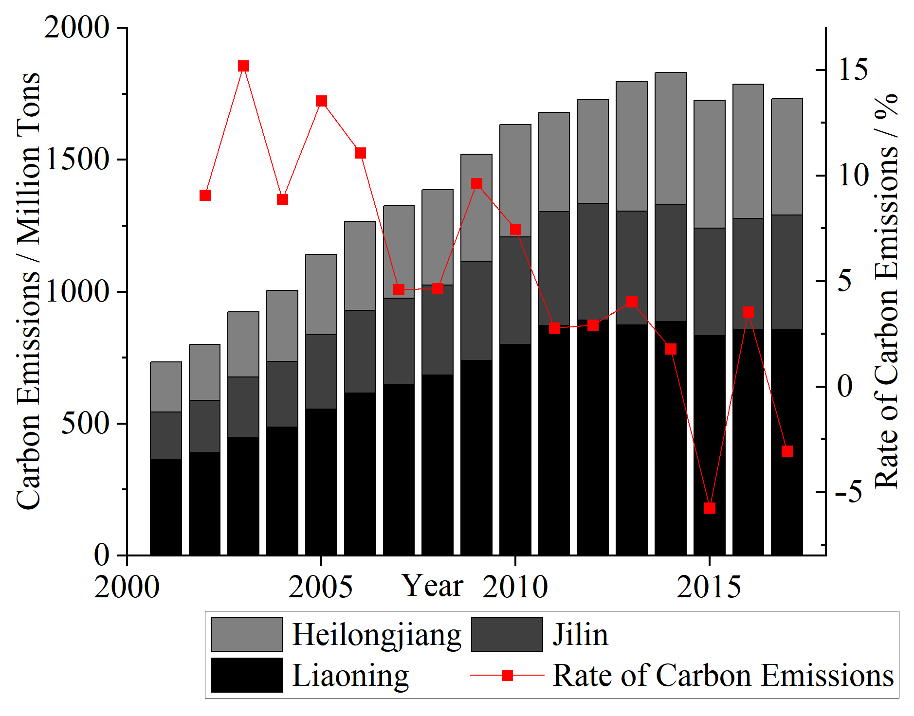
Figure 3.
Moran’s I index of carbon emissions in the three northeastern provinces.

Figure 4.
Local indicators of spatial association.

Figure 5.
Spatial distribution of city types.

Figure 6.
Descriptive statistics of Theil index based on total carbon emissions.


Table 1.
Comparison of analysis methods.
| Method | Advantages | Disadvantages | Application in Carbon Emission Field |
|---|---|---|---|
| Linear regression model | Understandable and straightforward: easy to comprehend and explain. High computational efficiency: fast model training and prediction with a low demand on computational resources. | Model assumption limitations: it assumes linear relationships, is sensitive to outliers, and is unsuitable for nonlinear relationships. | Fundamental in regression analysis. Scholars widely use this model as an initial model to analyze factors affecting carbon emissions and for comparisons with other models [26,27]. |
| Random forest regression model | Handles non-linearity: effectively manages non-linear relationships and high-dimensional interactions. Robust: insensitive to outliers and noise but has strong generalization capability. Feature importance assessment: provides importance scores for variables, aiding in understanding their contributions to the model. | High computational complexity: requires substantial computing resources, especially with large datasets. Poor interpretability: as a black-box model, its decision-making process is difficult to explain. | It is commonly used for the time series prediction of carbon emissions or to identify the importance of influencing factors [28,29]. |
| Shapley additive explanations | High interpretability: detailed explanation of each feature’s contribution to model predictions through SHAP values. Model universality: Applicable to any machine learning model, enhancing transparency and credibility. | High computational cost: particularly with many features, computing SHAP values can be very time-consuming. Complex implementation: Requires high technical proficiency for correct implementation and interpretation. | It is relatively new, with details and uses still under discussion. However, it allows for a better assessment of the contributions and thresholds of factors influencing carbon emissions [30]. |
| Geographically weighted regression | Models spatial heterogeneity: can model and explain spatial variability in data. Enhances local prediction accuracy: improves local fitting accuracy in spatial data analysis. | High data demand: requires sufficient spatial data for local estimation. Potential for overfitting: prone to overfitting in areas with dense data points or small regions. | It is often used to characterize the spatial heterogeneity features of carbon emissions from industries, households, and other spatial elements [31,32]. |
| Geographic detector | Detects interactions: Effectively identifies interactions between different factors and their impact on the target variable. No model assumptions: these are not based on prior statistical model assumptions and are suitable for various data types. | Limited interpretability: only determines whether a significant relationship exists between factors and cannot identify precise relationship forms. Sensitive to data quality: the results depend on data completeness and quality. | It is commonly used in areas with significant stratified heterogeneity for carbon emission analysis [33,34]. |
| Spatial econometric model | Handles spatial dependencies: effectively manages spatial autocorrelation and heterogeneity, improving estimation accuracy. Solid theoretical foundation: provides rich theoretical support for understanding and analyzing the complex dynamics of spatial data structures. | Complex model setup: the selection of a spatial weight matrix and parameter setting require expertise. High computational demands: a large computational load on large datasets, which may need specialized software and hardware. | It is frequently used in urban carbon emission studies to scientifically measure spatial dependencies and effects [35,36]. |
Table 2.
Data descriptions.
| Influencing Factors | Abbreviation |
|---|---|
| Gross domestic product | GDP, x1 |
| Population scale | PS, x2 |
| General public budget revenue | GPBR, x3 |
| General public budget expenditure | GPBE, x4 |
| Construction land area | CLA, x5 |
| Output value of secondary industries | SSI, x6 |
| Output value of tertiary industries | STI, x7 |
| Gross domestic product per capita | GDPPC, x8 |
| Fixed asset investment | FAI, x9 |
Table 3.
The judgment matrix for shrinking cities.
| Cumulative Count of Population Decreases/c | Rate of Population Size Change/r | Type |
|---|---|---|
| 9 ≤ c | r < 0 | Shrinking cities |
| 0 ≤ r | ||
| 0 ≤ c < 9 | r < 0 | Shrinking cities |
| 0 ≤ r | Growing cities |
Table 4.
MK trend test.
| Province | Sen’s Slope | z-Value | p-Value |
|---|---|---|---|
| Jilin | 19.96 *** | 4.33 | 1.52 × 10⁻⁵ |
| Liaoning | 9.46 *** | 4.41 | 1.05 × 10⁻⁵ |
| Heilongjiang | 10.61 *** | 4.74 | 2.17 × 10⁻⁶ |
| Total | 38.91 *** | 4.90 | 9.49 × 10⁻⁷ |
*** indicates significant performance at a 1% confidence level.
Table 5.
Bidirectional statistics of city types.
| Province | Growing Cities | Proportion (%) | Shrinking Cities | Proportion (%) | Total |
|---|---|---|---|---|---|
| Jilin | 25 | 43.10 | 33 | 56.90 | 58 |
| Liaoning | 51 | 52.04 | 47 | 47.96 | 98 |
| Heilongjiang | 58 | 50.00 | 58 | 50.00 | 116 |
| Total | 134 | 49.27 | 138 | 50.74 | 272 |
Table 6.
Difference test for total carbon emissions between growing and shrinking cities.
| Test Method | Shrinking Cities | Growing Cities | Difference Value |
|---|---|---|---|
| Mean test | 3.10 | 2.11 | 0.99 *** |
| Median test | 2.37 | 1.66 | 115.90 *** |
*** indicates significant performance at a 1% confidence level.
Table 7.
Panel regression estimations and test results.
| Factors | (1) | (2) | (3) |
|---|---|---|---|
| Total | Growing Cities | Shrinking Cities | |
| GDP, x1 | 0.25 *** | 0.20 *** | 0.27 *** |
| (0.04) | (0.05) | (0.06) | |
| PS, x2 | 0.04 | 0.41 | −1.41 *** |
| (0.29) | (0.46) | (−0.47) | |
| GPBR, x3 | 0.02 | 0.02 | 0.02 * |
| (0.02) | (0.02) | (0.01) | |
| GPBE, x4 | −0.04 *** | −0.01 | −0.05 ** |
| (−0.02) | (−0.02) | (−0.02) | |
| CLA, x5 | 0.37 ** | 0.58 ** | 0.11 |
| (0.18) | (0.29) | (0.09) | |
| SSI, x6 | −0.09 *** | −0.08 ** | −0.10 *** |
| (−0.03) | (−0.04) | (−0.04) | |
| STI, x7 | −0.26 *** | −0.29 *** | −0.07 ** |
| (−0.06) | (−0.06) | (−0.04) | |
| GDPPC, x8 | 0.01 | 0.05 ** | −0.07 ** |
| (0.02) | (0.02) | (−0.05) | |
| FAI, x9 | 0.04 * | 0.05 * | 0 |
| (0.02) | (0.02) | (0.02) | |
| N | 3417 | 1802 | 1615 |
| AIC | −1243.70 | −56.11 | −1938.30 |
| BIC | −1090.30 | 81.31 | −1803.60 |
The parentheses indicate the corresponding standard error; *, ** and *** indicate significance at confidence levels of 10%, 5%, and 1%, respectively.
Table 8.
Estimation results of panel spatial Dubin model.
| Factors | (4) | (5) | (6) |
|---|---|---|---|
| Total | Growing Cities | Shrinking Cities | |
| GDP, x1 | 0.19 *** | 0.11 *** | 0.43 *** |
| (0.01) | (0.02) | (0.02) | |
| PS, x2 | 0.42 *** | 0.59 *** | 0.80 *** |
| (0.08) | (0.14) | (0.14) | |
| GPBR, x3 | 0.02 *** | 0.02 *** | 0.02 *** |
| (0) | (0.01) | (0.01) | |
| GPBE, x4 | 0.01 * | 0.03 ** | 0 |
| (0.01) | (0.01) | (0.01) | |
| CLA, x5 | 0.62 *** | 0.97 *** | 0.21 *** |
| (0.04) | (0.07) | (0.03) | |
| SSI, x6 | −0.08 *** | −0.07 *** | −0.13 *** |
| (−0.01) | (−0.01) | (−0.02) | |
| STI, x7 | −0.23 *** | −0.24 *** | −0.08 *** |
| (−0.01) | (−0.01) | (−0.02) | |
| GDPPC, x8 | 0.01 | 0.04 *** | −0.15 *** |
| (0.01) | (0.01) | (−0.02) | |
| FAI, x9 | 0.06 *** | 0.06 *** | 0.01 |
| (0.01) | (0.01) | (0.01) | |
| W×GDP, W×x1 | 0.03 | 0.08 ** | −0.05 |
| (0.02) | (0.03) | (−0.04) | |
| W×PS, W×x2 | −0.60 *** | −0.84 *** | −0.40 * |
| (−0.16) | (−0.29) | (−0.23) | |
| W×GPBR, W×x3 | 0 | 0.02 | −0.01 |
| (0.01) | (0.01) | (−0.01) | |
| W×GPBE, W×x4 | −0.13 *** | −0.17 *** | −0.03 ** |
| (−0.02) | (−0.03) | (−0.01) | |
| W×CLA, W×x5 | −0.98 *** | −1.12 *** | −0.58 *** |
| (−0.09) | (−0.14) | (−0.08) | |
| W×SSI, W×x6 | 0.06 *** | 0.05 ** | 0.26 *** |
| (0.02) | (0.03) | (0.04) | |
| W×STI, W×x7 | 0.02 | −0.01 | 0.10 *** |
| (0.02) | (−0.03) | (0.03) | |
| W×GDPPC, W×x8 | −0.02 | −0.03 | −0.10 *** |
| (−0.02) | (−0.02) | (−0.03) | |
| W×FAI, W×x9 | −0.02 * | −0.02 | −0.05 ** |
| (−0.01) | (−0.02) | (−0.02) | |
| rho | 0.29 *** | 0.27 *** | 0.26 *** |
| (0.03) | (0.04) | (0.03) | |
| N | 3417 | 1802 | 1615 |
| AIC | −1714.20 | −271.38 | −2179.76 |
| BIC | −1481.01 | −62.51 | −1975.05 |
The parentheses indicate the corresponding standard error; *, ** and *** indicate significance at confidence levels of 10%, 5%, and 1%, respectively.
Table 9.
Effect decomposition of panel spatial Dubin model.
| Factors | (4) | (5) | (6) | |
|---|---|---|---|---|
| Total | Growing Cities | Shrinking Cities | ||
| Direct effects | GDP, x1 | 0.20 *** | 0.12 *** | 0.43 *** |
| (0.01) | (0.02) | (0.02) | ||
| PS, x2 | 0.40 *** | 0.56 *** | −0.83 *** | |
| (0.08) | (0.14) | (−0.14) | ||
| GPBR, x3 | 0.02 *** | 0.02 *** | 0.02 *** | |
| (0) | (0.01) | (0.01) | ||
| GPBE, x4 | 0.01 | 0.03 ** | 0 | |
| (0.01) | (0.01) | (0.01) | ||
| CLA, x5 | 0.58 *** | 0.93 *** | 0.18 *** | |
| (0.03) | (0.06) | (0.03) | ||
| SSI, x6 | −0.08 *** | −0.07 *** | −0.11 *** | |
| (−0.01) | (−0.01) | (−0.02) | ||
| STI, x7 | −0.24 *** | −0.24 *** | −0.08 *** | |
| (−0.01) | (−0.01) | (−0.02) | ||
| GDPPC, x8 | 0.01 | 0.04 *** | −0.15 *** | |
| (0.01) | (0.01) | (−0.02) | ||
| FAI, x9 | 0.06 *** | 0.06 *** | 0 | |
| (0.01) | (0.01) | (0.01) | ||
| Indirect effects | GDP, x1 | 0.12 *** | 0.15 *** | 0.07 |
| (0.03) | (0.04) | (0.05) | ||
| PS, x2 | −0.65 *** | −0.89 ** | −0.78 *** | |
| (−0.2) | (−0.38) | (−0.28) | ||
| GPBR, x3 | 0.01 | 0.03 * | −0.01 | |
| (0.01) | (0.02) | (0.01) | ||
| GPBE, x4 | −0.17 *** | −0.21 *** | −0.04 ** | |
| (−0.02) | (−0.04) | (−0.02) | ||
| CLA, x5 | −1.10 *** | −1.14 *** | −0.68 *** | |
| (−0.12) | (−0.17) | (−0.1) | ||
| SSI, x6 | 0.05 * | 0.05 | 0.29 *** | |
| (0.03) | (0.03) | (0.05) | ||
| STI, x7 | −0.07 ** | −0.09 ** | 0.10 ** | |
| (−0.03) | (−0.04) | (0.04) | ||
| GDPPC, x8 | −0.03 | −0.03 | −0.18 *** | |
| (−0.02) | (−0.03) | (−0.04) | ||
| FAI, x9 | 0 | 0 | −0.06 ** | |
| (0.02) | (0.02) | (−0.03) | ||
The parentheses indicate the corresponding standard error; *, ** and *** indicate significance at confidence levels of 10%, 5%, and 1%, respectively.
Disclaimer/Publisher’s Note: The statements, opinions and data contained in all publications are solely those of the individual author(s) and contributor(s) and not of MDPI and/or the editor(s). MDPI and/or the editor(s) disclaim responsibility for any injury to people or property resulting from any ideas, methods, instructions or products referred to in the content. |
© 2024 by the authors. Licensee MDPI, Basel, Switzerland. This article is an open access article distributed under the terms and conditions of the Creative Commons Attribution (CC BY) license (https://creativecommons.org/licenses/by/4.0/).
Share and Cite
MDPI and ACS Style
Song, Y.; Tian, J.; He, W.; Namaiti, A.; Zeng, J. Differential Analysis of Carbon Emissions between Growing and Shrinking Cities: A Case of Three Northeastern Provinces in China. Land 2024, 13, 648. https://doi.org/10.3390/land13050648
AMA Style
Song Y, Tian J, He W, Namaiti A, Zeng J. Differential Analysis of Carbon Emissions between Growing and Shrinking Cities: A Case of Three Northeastern Provinces in China. Land. 2024; 13(5):648. https://doi.org/10.3390/land13050648
Chicago/Turabian StyleSong, Yuanzhen, Jian Tian, Weijie He, Aihemaiti Namaiti, and Jian Zeng. 2024. "Differential Analysis of Carbon Emissions between Growing and Shrinking Cities: A Case of Three Northeastern Provinces in China" Land 13, no. 5: 648. https://doi.org/10.3390/land13050648
Note that from the first issue of 2016, this journal uses article numbers instead of page numbers. See further details here.