

Tomographic Background-Oriented Schlieren for Axisymmetric and Weakly Non-Axisymmetric Supersonic Jets

1
Key Laboratory of Fluid Mechanics of Ministry of Education & Aircraft and Propulsion Laboratory, Ningbo Institute of Technology, Beihang University, Beijing 100191, China
2
School of Aerospace Engineering, Huazhong University of Science & Technology, Wuhan 430074, China
3
Tianmushan Laboratory, Xixi Octagon City, Yuhang District, Hangzhou 310023, China
*
Author to whom correspondence should be addressed.
†
These authors contributed equally to this work.
Symmetry 2024, 16(5), 596; https://doi.org/10.3390/sym16050596
Submission received: 8 April 2024
/
Revised: 30 April 2024
/
Accepted: 6 May 2024
/
Published: 11 May 2024
(This article belongs to the Special Issue Applications Based on Symmetry/Asymmetry in Fluid Mechanics)
Abstract
:The Schlieren technique is widely adopted for visualizing supersonic jets owing to its non-invasiveness to the flow field. However, extending the classical Schlieren method for quantitative refractive index measurements is cumbersome, especially for three-dimensional supersonic flows. Background-oriented Schlieren has gained increasing popularity owing to its ease of implementation and calibration. This study utilizes multi-view-based tomographic background-oriented Schlieren (TBOS) to reconstruct axisymmetric and weakly non-axisymmetric supersonic jets, highlighting the impact of flow axisymmetry breaking on TBOS reconstructions. Several classical TBOS reconstruction algorithms, including FDK, SART, SIRT, and CGLS, are compared quantitatively regarding reconstruction quality. View spareness is identified to be the main cause of degraded reconstruction quality when the flow experiences axisymmetry breaking. The classic visual hull approach is explored to improve reconstruction quality. Together with the CGLS tomographic algorithm, we successfully reconstruct the weakly non-axisymmetric supersonic jet structures and confirm that increasing the nozzle bevel angle leads to wider jet spreads.
1. Introduction
Jet propulsion systems play a pivotal role in aviation and aerospace. These systems are based on the momentum theorem, and the core mechanism for generating propulsion is to accelerate the exhaust of high-pressure gas so that the aircraft or rocket obtains reacting force. The high-speed exhaust forms a supersonic jet and produces complex flow structures such as shock waves, expansion waves, and shear flow under the influence of the boundary conditions of the nozzle and the ambient atmosphere. These flow structures significantly impact the propulsion performance and jet noise emissions, thus requiring further in-depth research.
The state of the supersonic jet depends on the relationship between the total pressure at the nozzle outlet and the ambient pressure. It can be characterized by the nozzle pressure ratio (NPR) shown in the following equation:
Inside and are the stagnation pressure of the jet and the ambient pressure, respectively; represents the jet Mach number, and is the specific heat ratio. The jet of aero and rocket engines is usually in an under-expansion state; that is, its is greater than the designed Mach number of the nozzle so that the jet can gain higher momentum. Many studies have explored the impact of complex flow structures such as shock reflection, shock hysteresis, and nozzle flow separations on supersonic jet performance [1,2,3,4].
Supersonic jets are also the main noise sources of aircraft, which produce turbulent mixing noise, broadband shock-associated noise, and screech tones [5,6,7]. Some studies have pointed out that enhancing the mixing of jets with surrounding fluids can significantly alleviate turbulent mixing noise and shock-associated noise, and many methods for promoting low-speed jet mixing have been developed [8,9,10,11]. However, due to the significant compressibility effect, effectively mixing supersonic jets with ambient flows is not trivial. Appropriate modification of the nozzle trailing edge is a method that has been widely studied to enhance the mixing of supersonic jets. The extended perimeter of the trailing edge will facilitate the interaction between high-speed and low-speed flows [12,13,14]. Wu and New [15] studied single-beveled nozzles and observed changes in the shock cell structure caused by the presence of the nozzle notch, and the beveled nozzle shortened the potential core length, indicating better jet mixing capabilities. Rice and Raman [16] found that compared with the single-beveled nozzle, a double-beveled nozzle with a more symmetrical geometry can produce a more symmetrical jet and may provide better mixing performance. Raman [17] studied the shock cell structure and the noise of beveled rectangular jets, and they noted that jets produced by inclined notches generally produce weak screech tones over a limited range of Mach numbers.
Further improvements in the propulsion system require a detailed and accurate three-dimensional description of the supersonic jet flow structures. The compressibility of supersonic flow causes its density to change, and according to the Gladstone–Dale relation (), the gas index of refraction (IOR, n) is proportional to its density (assuming that the G–D constant K of air is constant). Therefore, the flow structures can be characterized by the IOR distribution of the flow field. The classical Schlieren method uses this feature of the compressible flow to visualize supersonic flow fields. The background-oriented Schlieren (BOS) method was proposed around 2000 [18,19], and due to the advantages of simple optical design and low implementation cost, it has been widely used in the two-dimensional (2D) measurement of supersonic jets [20,21].
Tomographic background-oriented Schlieren (TBOS), which combines tomography with BOS measurement, makes it possible to measure three-dimensional (3D) non-uniform density fields. Abel inversion was first applied to the reconstruction of axisymmetric flow fields [22,23]. Later, Venkatakrishnan and Meier [24] proposed using the Filtered Back Projection (FBP) algorithm to reconstruct the axisymmetric density field to avoid the algorithm singularities and noise sensitivity of Abel inversion. Tan et al. [25] successfully implemented the density field measurement of axisymmetric supersonic jets using the adaptive Fourier–Hankel (AFH) methods. Xiong et al. [26] compared the onion peeling (OP), three-point Abel (TPA), FBP, and AFH methods and found that, in the presence of noise, the three-point Abel inversion yielded the best axisymmetric IOR reconstruction results. Facing the reconstruction of the more general 3D supersonic jet, multi-view BOS measurement is required. Kirby [27] reported the use of TBOS technology to measure supersonic jets generated by elliptical nozzles, which study used BOS observations of 40 views and the FBP-SART combined algorithm; although his results restored flow structures such as shocks to a certain extent, errors and artifacts are still evident. Nicolas et al. [28] used the least squares optimization algorithm and spatial mask constraints to achieve axisymmetric under expanded supersonic jet reconstruction with fewer than 20 viewing angles. However, achieving high-quality flow reconstruction for non-axisymmetric supersonic jets with sparse camera views remains challenging.
In this paper, we systematically investigated the application of TBOS reconstruction to under-expansion supersonic jets with/without axisymmetry breaking. The paper is organized as follows: Section 2 outlines the measurement principle of TBOS, the tomographic reconstruction algorithm, and virtual device settings used subsequently; Section 3 studies the reconstruction of the jet structures transitioning from axisymmetry to weak non-axisymmetry, focusing on the impact of algorithms, noise, and visual-hull-like mask methods on reconstruction, and the physics of jets are discussed; and Section 4 provides the main conclusions of this study.
2. Methodology
2.1. Principle of TBOS
The TBOS principle has been discussed in detail in previous studies [29,30], so it is only briefly introduced here. As shown in Figure 1, the X point on the background pattern is mapped to the Y point on the imaging plane after passing through the space of constant IOR; however, in the presence of a flow field with non-uniform IOR, the light ray is deflected and mapped on Y′. At this time, the optical path can be described by the following ray equation:
where represents the coordinates of a certain point on the optical path, represents the differential length, and represents the local refractive index gradient. This equation can be rewritten as follows:
where represents the ray vector. For a gas environment with , can be approximated as a unit vector. Therefore, the deflection of a light ray passing through the entire non-uniform IOR region is defined as the integral of along the optical path S:
where and represent the direction vectors of a light ray entering and leaving the flow field, respectively. In the actual BOS experiment, the background pattern is first imaged to obtain the Y position under a uniform IOR condition. The imaging settings are kept unchanged and performed in the presence of non-uniform IOR. Based on this pair of images and the cross-correlation algorithm or the optical flow method [31], the imaging/pixel displacement is calculated, and . Finally, through simple geometric optics calculations, the approximate and and deflection can be obtained. For a multi-camera TBOS measurement, through imaging with multiple view angles and further discretizing Equation (4), we can obtain the following:
The inside subscript u represents the directions . The multi-camera imaging determines I rays, and the measurement volume contains a total of J discrete voxels. Then represents the vector of all ray deflections; is a vector recording all IOR gradients; and is the tomographic coefficient matrix, in which the elements marked by record the contribution weight of of the j-th voxel to the deflection of the i-th ray. Obviously, Equation (5) forms a large linear system of equations in the form . Solving x, that is, in Equation (5), is to solve the inverse problem of linear equations.
2.2. Tomographic Reconstruction Algorithm
Under a limited observation angle, the sampled I (number of effective rays) is usually much smaller than J. Furthermore, Equation (5) is seriously ill-posed due to measurement errors and noise. Therefore, the direct inversion method cannot solve the tomographic reconstruction problem. Still, some numerical solution techniques must be used to estimate a solution as close to the true value as possible.
Many algorithms have been used for tomographic reconstruction, driven by multiple disciplines, such as computed tomography and magnetic resonance imaging. Based on the principle of solving, tomography reconstruction algorithms are mainly divided into analytical and iterative types. The analytical algorithm is based on the mathematical model of the measurement system and is directly calculated analytically. Iterative algorithms are based on statistical models of measured data, using iterative optimization operations to estimate the best reconstructions. The two types of reconstruction algorithms have specific characteristics, so during TBOS reconstruction, they must be selected based on objective conditions and requirements.
When the flow field to be measured has the characteristics of axisymmetry, it can be considered that the BOS measurements performed around the symmetry axis are the same. Therefore, only the BOS measurement of one view is needed to carry out the tomographic reconstruction of any multiple view angles. Currently, the number of effective rays (I in Equation (5)) can be increased without limit, making the system of equations close to a positive definite state. In this case, analytical algorithms, such as Abel transform, AFH, and FBP, can be used for reconstruction. Multi-view measurements are required for the TBOS reconstruction of a non-axisymmetric flow field. However, the number of observation view angles (projection planes) is limited due to laboratory space and equipment costs. In this case, iterative algorithms show better reconstruction results in practice. For a detailed introduction to various volume tomography reconstruction algorithms, please refer to the review by Grauer et al. [32]. The following is a brief introduction to the tomographic reconstruction algorithm used in this paper.
2.2.1. Analytical Algorithm
FBP is currently the most widely used analytical reconstruction algorithm. Its basis is the Fourier central slice theorem [33]: If a 3D measured target x is imaged from different viewing angles, a series of 2D projections b can be obtained; the 1D Fourier transform of these projections b is equal to the slice of the 2D Fourier transform of x at the corresponding viewing angle. Therefore, when enough views of b are sampled, the slices can be combined into a complete 2D Fourier transform of x, and finally, the reconstruction of x can be completed through the inverse Fourier transform. Another necessary operation of FBP is performing convolution filtering on the Fourier transformed b to eliminate the measurement error and the noise diffusion. Therefore, the reconstruction process of FBP can be summarized as follows:
- Perform a 1D Fourier transform on the projection data.
- Select appropriate filters to perform convolutional filtering on the transformed projection.
- Back-project the filtered projection data into the measurement volume.
- All back projections are superimposed to obtain the reconstructed projection.
The traditional FBP algorithm can only process projection data under parallel beam and uniform distribution conditions, so it cannot be directly applied to TBOS reconstruction based on the camera imaging model (cone beam) and arbitrary viewing angle sampling. We use the improved FBP algorithm proposed by Feldkamp, Davis, and Kress, also known as the FDK algorithm [34]. It introduces a more complex reconstruction geometric model and overcomes the limitations of FBP through weighted correction in the operation. In addition, the Ram-Lak filter is used in the current FDK algorithm, which is equivalent to an ideal high-pass filter in the frequency domain, so it can remove low-frequency information and enhance high-frequency information, thereby highlighting the flow structure.
2.2.2. Iterative Algorithm
The algebraic reconstruction technique (ART) is the most commonly used iterative algorithm family. It was originally used to replace the FBP algorithm and outperforms FBP in the case of fewer projections. For inverse problems of the form , the ART follows the following iteration structure:
where is the relaxation coefficient used to control the convergent speed of iteration, and V and W are weight matrices based on the length of the light ray. The basic ART algorithm sequentially calculates (-th row of A, corresponding to one ray) and projection to update x and completes an iteration after traversing all rays.
To improve computational efficiency and robustness, modified ART algorithms such as SART and SIRT [35] emerged: the SART algorithm updates x by projection planes one by one, while SIRT uses all projection planes to update. Generally, the more data are used in an update, the faster each iteration step will be, but the slower the convergence (more iterations) will be. The current study uses these two algorithms, and the relaxation coefficients are all set to .
Another type of iterative algorithm is performing optimization operations on Equation (7) under the least squares framework to obtain the reconstruction result with the highest probability. This method is derived from the statistical model based on the TBOS system and measurement data.
This paper used the CGLS [36] algorithm for the above problem, which is a derivative iterative algorithm of Krylov methods: at the -th iteration, the optimal solution belonging to the Krylov subspace of increasing dimensions is found according to the optimality criterion defined by the specific Krylov solver. Krylov subspaces are linear combinations of matrices’ first powers acting on vectors. In the tomographic reconstruction problem, we mainly focus on the subspace of acting on , as shown in the following equation:
CGLS uses the conjugate gradient method to find the fastest descent direction. Therefore, the result of the -th iteration is the least square solution under the -order Krylov subspace:
which can make the residual statistics monotonically decrease. Algorithm 1 below shows the simplified CGLS process.
It is apparent that FDK, utilizing the Fourier central slice theorem, circumvents the cumbersome iterative process by directly deriving the reconstruction result from projection data. Consequently, FDK offers a significantly faster computational speed, which is widely acknowledged as one of its primary advantages. In contrast, iterative algorithms necessitate continuous projection and back-projection operations to iteratively minimize the final residual. As a result, they incur higher computational loads and usually require more time to accomplish the reconstruction process.
| Algorithm 1 CGLS |
| Initialize: for do end for Output: |
2.3. Experimental Setting
In this paper, we adopted an experimental scheme of TBOS measurement based on CFD data and a synthetic BOS image generation platform [37]. Its process was as follows: the target flow fields were computed via CFD simulation, the flow field data were incorporated within the ray-tracing process of synthetic BOS image generation, and then the background pattern imaging was performed through ray tracing technology, and the synthetic BOS images were used for tomographic reconstruction studies. Because of the existence of CFD data as the ground truth, this scheme has the advantage of quantifiable algorithm accuracy.
This paper studied the under-expanded jets produced by three types of nozzles, as shown in Figure 2. These nozzles had the same parameters: the internal diameter ( mm), the total length (i.e., average of the shortest and longest axial lengths), and the design Mach number (). Three-dimensional Reynolds-averaged Navier-Stokes (RANS) simulations were conducted for these nozzles, assuming that the supersonic shock structure was quasi-steady. The ANSYS CFX solver was used to simulate arbitrary flow scenarios involving complex physical geometries under low- and high-speed conditions [38,39]. To ensure the stability of the numerical simulations, shock and expansion waves were captured via a high-resolution advection scheme. The jets of the three nozzles were all set to , and the corresponding Mach number was 1.56. For more detailed nozzle and CFD simulation settings, please refer to previous research [40].
Figure 3 shows the configuration for generating the synthetic BOS images. The cameras adopted an annular coplanar arrangement with the nozzle center as the axis, and the supersonic jet was located between the camera and the background pattern. Lang et al. [41] discussed the impact of the number and distribution of BOS camera views on reconstruction accuracy and concluded that odd-numbered views and coplanar annular arrangements can achieve optimal results. At the same time, arranging dozens of cameras in actual experiments is usually not feasible. Therefore, we referred to the studies of Atcheson et al. [42] and Nicolas et al. [28], and used 15 cameras/BOS in the present work. Under this measurement setting, we synthesized multi-view BOS images through ray tracing technology, and their resolution was pixels. The data of pixel displacement were obtained through an in-house optical flow method [43]. The inquiry window size was set to pixels, so the resolution of the field was (Figure 4a). Further, the deflection required for the tomographic reconstruction operation, as shown in Figure 4b, can be obtained. Table 1 lists the detailed parameters of the TBOS device and data processing.
3. Results and Discussion
3.1. Axisymmetric Jet Flow
We investigate the reconstruction of an under-expanded jet from the non-beveled nozzle. Considering its special axisymmetric structure, all projection planes are identical within the annular region. Therefore, only one projection plane was utilized to simulate the projection planes obtained from 180 viewing angles. Figure 5 illustrates the spatial distribution of obtained from CFD and reconstruction data. Observational analysis was performed on two selected cross-sections from the radial and flow direction positions. Figure 6 compares at two sampling positions marked in Figure 5. Note that the dashed line ② is not strictly linear but represents a series of points with maximum selected successively along the flow direction.
First, as depicted in Figure 5, it can be observed that the reconstruction results from four algorithms effectively identify the primary flow structures of the supersonic jet. Moreover, except for the SIRT algorithm, which captures comparatively lower peak values of , the remaining algorithms reconstruct profiles matching the ones from CFD well.
Figure 6a illustrates that FDK attains superior reconstruction accuracy at the peaks of , with specific peak errors delineated in Table 2. However, its capability to capture peak values in the downstream region might slightly lag behind that of SART and CGLS, as portrayed in Figure 6b. Besides peak errors, we also factor in their computation time and utilize the root mean square error (RMSE, Equation (10)) to evaluate the overall reconstruction quality of the algorithms, as illustrated in Table 2. Benefiting from its analytical reconstruction nature, which circumvents cumbersome iterative processes, FDK enjoys a clear advantage in computation time. Conversely, SART frequently demands more time during reconstruction due to its nested iterative loop. Considering these aspects holistically, it becomes apparent that FDK ensures high-quality reconstruction outcomes and meets the demand for swift reconstruction.
3.2. Non-Axisymmetric Jet Flow
3.2.1. Weakly Non-Axisymmetric Jet Flow
Next, we consider the reconstruction of a non-axisymmetric under-expanded jet using the double-beveled nozzle. Due to the axisymmetry breaking in the jet flow structure, tomographic reconstruction necessitates multi-view BOS measurements, i.e., projections. As Section 2.3 outlined, we utilized 15 projections in the current scenario. Similarly, we applied the method described in the preceding subsection to analyze the reconstruction outcomes.
In this scenario, the limited projection data noticeably affect all reconstruction algorithms. As depicted in Figure 7, there is a significant decrease in the overall quality of the reconstruction results. On the one hand, noticeable streak artifacts appear in the reconstruction results, especially in the outer regions of the flow field. On the other hand, the algorithm’s ability to capture the peak of is affected, with the iterative reconstruction algorithms demonstrating inferior performance.
Through specific numerical analysis, clear differences can be observed in the reconstruction results between analytical and iterative algorithms. Table 2 provides a comprehensive assessment of the overall reconstruction performance of these algorithms, indicating that although FDK retains a notable advantage in computation time, its overall reconstruction error is considerably higher compared with the iterative algorithms. The three iterative algorithms produce nearly identical reconstruction results, with the CGLS algorithm exhibiting significantly shorter computation time.
The disparity in is depicted in Figure 8a. The variation of from the center to the outer regions of the jet indicates a decreasing level of consistency between the reconstruction results of the four algorithms and the CFD data. Particularly noticeable are significant fluctuations near the edges of the flow field, with this phenomenon being especially prominent in the reconstruction results obtained with FDK. The red box in Figure 8a highlights the superior artifact suppression capabilities of the iterative algorithms compared with FDK, which contributes to the higher RMSE observed in the FDK results (as indicated in Table 2). Figure 8b analyzes the variation of the peak of along the flow direction. Despite being influenced to some extent, FDK still manages to capture the peak of effectively. This advantage is particularly evident in regions of high gradients upstream of the jet. The zoomed-in sections in Figure 8a,b illustrate that CGLS demonstrates the superior peak of capturing capabilities compared other iterative algorithms. Furthermore, Figure 8b indicates that, in the downstream region of the flow, the impact of artifacts on these four algorithms is minimal and the reconstructed results are generally consistent with CFD data, effectively capturing the flow characteristics of the jet.
In summary, while FDK demonstrates efficient computation time and effective capturing of the peak of , it falls short in artifact suppression and overall reconstruction quality compared with iterative algorithms.
From the above reconstruction results, it is evident that the limited projection data cannot adequately facilitate the accurate reconstruction of non-axisymmetric jets, which is the main adverse effect of axisymmetry breaking on TBOS reconstruction. Currently, Equation (5) is seriously ill-posed. Without altering the experimental settings, one feasible approach to improve the reconstruction quality is constraining Equation (5) by utilizing prior information acquired through a comparative analysis between the reconstruction results and CFD data.
3.2.2. Visual Hull Technique
To ensure the completeness of the data in the test area, the typically employed reconstruction volume is a parallelepiped, covering the entire region of the test flow field. There are typically no significant changes in the refractive index in regions outside the flow field. Consequently, when the ray propagates along its whole path that does not intersect regions with , it will not undergo deviation, resulting in no in the imaging plane. However, during the tomographic reconstruction, it is inevitable that voxels without will receive some numerical allocation, leading to artifacts such as those observed in the reconstruction results depicted in Figure 7. Utilizing this prior information, efforts can be made to systematically exclude voxels within these regions, thereby minimizing the number of unknowns that need to be solved. This strategic approach aims to alleviate the underdetermined nature of the problem under sparse view conditions, consequently improving solution accuracy. Such a methodology is similar to the visual hull technology in computer vision and finds widespread application in tomographic reconstruction [30,44].
The main idea of constructing the VH is performed as follows: By subjecting the acquired displacement field data (Figure 9a) to thresholding and other numerical image processing techniques, the regions devoid of pixel displacement are identified (Figure 9b), thereby facilitating the construction of a 2D silhouette. As the displacement data on the background pattern reflect integrated information of light ray deflections along the path, even in cases where no displacement information is observed on the background pattern, it cannot be conclusively inferred that no deflection occurred along the propagation path of the light ray. Therefore, the 2D silhouette is selected more conservatively in digital image processing.
Subsequently, all projection data containing the 2D silhouettes are individually back-projected onto the reconstruction volume subjected to binary encoding. The voxel values corresponding to the interior regions of the silhouette in the reconstruction volume are assigned as 1, while the voxel values corresponding to the exterior regions are assigned as 0. The summation of voxels at corresponding positions across these reconstruction volumes is conducted. Subsequently, voxels with a cumulative value of 15 after overlaying are identified as focal points for subsequent reconstruction algorithms, thereby eliminating a significant portion of voxels lying beyond the scope of the flow field region (based on prior information, of these voxels are assumed to be 0). Thus, we obtained a VH that closely conforms to the silhouette of the flow field, as depicted in Figure 9c.
3.2.3. Reconstruction Results with VH
In this section, we incorporate the VH into the reconstruction process to improve the reconstruction results. Based on the analysis of the results in Section 3.2.1, the well-performing FDK and CGLS will be utilized for the following research analysis. Likewise, we conduct a comparative analysis of the reconstruction results with the VH.
After employing the VH, the artifacts outside the flow field region in the reconstruction results have been effectively constrained, as depicted in Figure 10. However, residual artifacts persist within the reconstruction volume, particularly in the FDK reconstruction results. Furthermore, the VH enables the CGLS algorithm to better capture the peak of .
Figure 11 illustrates the quantitative improvement in reconstruction accuracy achieved by employing the VH with the two algorithms. Here, represents the deviation between the reconstruction results and CFD data, with lower numerical values indicating superior reconstruction results. In Figure 11a, the variation trend of along the radial direction of the jet is depicted. It is evident that the VH significantly suppresses artifacts in the external region of the flow field for both algorithms. Particularly noteworthy is the enhanced ability of CGLS to capture internal flow field data, especially the peak of . Incorporating the VH into CGLS brings the reconstruction results near the inner part and edge of the jet closer to the CFD data, albeit with subtle changes. Conversely, analyzing the variation of reconstruction results with the FDK algorithm, besides effectively suppressing artifacts in the external region of the flow field, there are no apparent changes in other regions. Figure 11b reflects the ability of reconstruction algorithms to capture the peak of along the flow direction. The improvement in this aspect is significant for the CGLS algorithm with the inclusion of the VH, whereas there is no benefit for FDK. However, the advantageous performance of the FDK algorithm in capturing the peak of is still evident, as reflected in the peak errors of FDK and CGLS combined with the VH, as shown in Table 2.
This observation can be attributed to the differences between the fundamental principles of FDK and the construction methodology of the VH. FDK conducts Fourier transformation on projection data and then back-projects them to reconstruct the volume. The flow field data within the 2D silhouettes mainly correspond to the flow field distribution in physical space. Therefore, the VH does not improve peak errors or reconstruction accuracy in the flow field region for FDK. Its primary function is to rigidly eliminate the influence of artifacts outside the flow field area. In contrast, for iterative algorithms, the VH can be conceptualized as forcibly reducing the weighting of voxels outside the region of interest during the reconstruction process. Consequently, voxels within the flow field region receive more numerical allocation during the iterative process, effectively enhancing the reconstruction quality of the flow field region while mitigating the impact of external artifacts.
In summary, employing the VH significantly improves the overall reconstruction accuracy of the algorithms. In such cases, it can be seen from Table 2 that the reconstruction qualities of the two algorithms are comparably close.
3.3. Noise Impact
During practical TBOS experiments, measuring noise is inevitable. For instance, when capturing background patterns with a camera, there may be a certain degree of noise, leading to discrepancies between the obtained displacement field data and the actual displacement data, ultimately impacting the results of the tomographic reconstruction. Therefore, we will consider the reconstruction results of the two algorithms when the projection data are polluted by noise. Here, we add Gaussian white noise following to the acquired displacement data, where , , resulting in of the noise amplitudes being within the range of . Three intensity ratios, , , and , are used in this work. The noisy is then used to generate the VH and tomographic reconstruction. It is important to note that a certain degree of filtering is necessary to reduce the impact of noise during the process of generating the VH.
The reconstructions using noisy displacement data are shown in Figure 12. It is obvious that when the noise intensity is low, both reconstruction algorithms are affected, but overall, they still achieve relatively good reconstruction results. As the noise intensity gradually increases to 5%, the reconstruction results of the FDK algorithm are severely affected, making it difficult to extract useful information. In contrast, although the CGLS algorithm is also significantly affected, it demonstrates better noise suppression than the FDK algorithm. Therefore, the CGLS algorithm exhibits better robustness, making it more conducive to reconstructing the target flow field in practical TBOS experiments. Here, we only briefly compared the robustness of the two algorithms in the presence of noise pollution in the data. Subsequently, different regularization methods will be employed to constrain the solving process for noise reduction. However, this aspect will not be extensively discussed in this paper.
3.4. Jet Flow Structure
This subsection will briefly compare the jet flows under different nozzles based on the reconstruction results. As shown in Figure 13, we include the jet flow from the double-beveled nozzle in addition to the previous reconstruction results. It can be observed that the main structures of the jet flow under different nozzle conditions are well reconstructed. Therefore, we can use this to analyze the jet flow structure briefly.
It can be observed that when there are double bevels, in the case of under-expanded jet flow, the upstream portion of the jet comes into contact with the surroundings earlier. Due to the higher jet flow static pressure, the transverse pressure relief accelerates the spread of the jet, leading to a transition of the jet cross-section from circular to elongated. As the bevel angle increases, this phenomenon becomes more pronounced. Therefore, compared with a circular nozzle, the jet flow from a double-beveled nozzle may be easier to control and adjust regarding jet direction.
At the same time, from the –slice in Figure 5 and Figure 7, it can be observed that, within the under-expanded jet flow, two shock waves appear internally. These shock waves undergo multiple reflections along the downstream potential core of the jet, resulting in prominent diamond shocks. It is foreseeable that these shocks will dissipate downstream with convection, while the shear layers of the jet will gradually merge at the end of the potential core. With the increase in bevel angle, it can be observed that the shear layers of the jet merge more rapidly, resulting in a shorter length of the potential core. This implies better jet mixing performance. Therefore, compared with jet flows from circular nozzles, jet flows from double-beveled nozzles can achieve better jet mixing performance.
4. Conclusions
This paper uses multi-view-based TBOS to reconstruct axisymmetric and weakly non-axisymmetric under expanded supersonic jets. Several classical TBOS reconstruction algorithms are compared quantitatively, including FDK, SART, SIRT, and CGLS. For axisymmetric jet flows, all algorithms except for SIRT achieve high-quality reconstruction, while FDK outperforms other methods in terms of reconstruction speed. For weakly non-axisymmetric jet flows, view sparseness leads to the emergence of prominent streak artifacts outside the reconstructed flow field regions. A significantly improved reconstruction quality can be achieved by imposing the VH during the reconstruction. Furthermore, CGLS outperforms the other methods in suppressing reconstruction artifacts, especially when there are strong noise contaminations. Finally, by analyzing the supersonic jet emanating from the double-beveled nozzle, TBOS measurements confirm that a double-beveled nozzle can induce a wider jet spread phenomenon and enhance jet mixing.
While we have considered the practical limitation on the number of cameras in TBOS experiments, in reality, the current number is still relatively high. Under more complex observation conditions, the actual number of cameras that can be used may not exceed 10, further affecting the experimental results. However, our current research has not yet conducted an in-depth analysis of this aspect. In future studies, attempts will be made to integrate more prior information about the flow to further optimize the reconstruction process, aiming to enhance the reconstruction quality under even sparser view conditions.
Author Contributions
Conceptualization, Y.X. and J.L.; methodology, J.L.; formal analysis, T.J.; data curation, T.J. and J.W.; writing—original draft preparation, T.J.; writing—review and editing, J.L., J.W., and Y.X.; funding acquisition, Y.X.; supervision, Y.X. All authors have read and agreed to the published version of the manuscript.
Funding
This research was funded by the National Natural Science Foundation of China (NSFC Grants No. 12102028).
Data Availability Statement
The data supporting this study’s findings are available from the corresponding author upon reasonable request.
Conflicts of Interest
The authors declare no conflicts of interest.
Abbreviations
The following abbreviations are used in this manuscript:
| NPR | nozzle pressure ratio |
| IOR | index of refraction |
| BOS | background-oriented Schlieren |
| TBOS | tomographic background-oriented Schlieren |
| FBP | Filtered Back Projection |
| FDK | Feldkamp, Davis, and Kress |
| ART | algebraic reconstruction technique |
| SART | Simultaneous Algebraic Reconstruction Technique |
| SIRT | Simultaneous Iterative Reconstruction Technique |
| CGLS | Conjugate Gradient Least Square |
| CFD | Computational Fluid Dynamics |
| RANS | Reynolds-Averaged Navier–Stokes |
| VH | visual hull |
References
- Hadjadj, A.; Kudryavtsev, A.N.; Ivanov, M.S. Numerical Investigation of Shock-Reflection Phenomena in Overexpanded Supersonic Jets. AIAA J. 2004, 42, 570–577. [Google Scholar] [CrossRef]
- Matsuo, S.; Setoguchi, T.; Nagao, J.; Alam, M.M.A.; Kim, H.D. Experimental study on hysteresis phenomena of shock wave structure in an over-expanded axisymmetric jet. J. Mech. Sci. Technol. 2011, 25, 2559–2565. [Google Scholar] [CrossRef]
- Schmisseur, J.D.; Gaitonde, D.V. Numerical simulation of Mach reflection in steady flows. Shock Waves 2011, 21, 499–509. [Google Scholar] [CrossRef]
- Shimshi, E.; Ben-Dor, G.; Levy, A. Numeric study of flow separation and shock reflection hysteresis in planar nozzles. Int. J. Aerosp. Innov. 2010, 2, 221–233. [Google Scholar] [CrossRef]
- Tam, C.K.W. Supersonic Jet Noise. Annu. Rev. Fluid Mech. 1995, 27, 17–43. [Google Scholar] [CrossRef]
- Tam, C.; Golebiowski, M.; Seiner, J. On the two components of turbulent mixing noise from supersonic jets. In Proceedings of the Aeroacoustics Conference, State College, PA, USA, 6–8 May 1996. [Google Scholar] [CrossRef]
- Raman, G. Supersonic jet screech: Half-century from powell to the present. J. Sound Vib. 1999, 225, 543–571. [Google Scholar] [CrossRef]
- Seiner, J.; Norum, T. Aerodynamic aspects of shock containing jet plumes. In Proceedings of the 6th Aeroacoustics Conference, Hartford, CT, USA, 4–6 June 1980. [Google Scholar] [CrossRef]
- Phanindra, B.C.; Rathakrishnan, E. Corrugated Tabs for Supersonic Jet Control. AIAA J. 2010, 48, 453–465. [Google Scholar] [CrossRef]
- New, T.H.; Tsovolos, D. Influence of nozzle sharpness on the flow fields of V-notched nozzle jets. Phys. Fluids 2009, 21, 084107. [Google Scholar] [CrossRef]
- Shi, S.; New, T.H. Some observations in the vortex-turning behaviour of noncircular inclined jets. Exp. Fluids 2013, 54, 1614. [Google Scholar] [CrossRef]
- Zaman, K.B.M.Q. Spreading characteristics of compressible jets from nozzles of various geometries. J. Fluid Mech. 1999, 383, 197–228. [Google Scholar] [CrossRef]
- Gutmark, E.J.; Schadow, K.C.; Yu, K.H. Mixing Enhancement in Supersonic Free Shear Flows. Annu. Rev. Fluid Mech. 1995, 27, 375–417. [Google Scholar] [CrossRef]
- Kim, J.H.; Samimy, M. Mixing enhancement via nozzle trailing edge modifications in a high speed rectangular jet. Phys. Fluids 1999, 11, 2731–2742. [Google Scholar] [CrossRef]
- Wu, J.; New, T.H. An investigation on supersonic bevelled nozzle jets. Aerosp. Sci. Technol. 2017, 63, 278–293. [Google Scholar] [CrossRef]
- Rice, E.; Raman, G. Mixing noise reduction for rectangular supersonic jets by nozzle shaping and induced screech mixing. In Proceedings of the 15th Aeroacoustics Conference, Long Beach, CA, USA, 25–27 October 1993. [Google Scholar] [CrossRef]
- Raman, G. Screech tones from rectangular jets with spanwise oblique shock-cell structures. J. Fluid Mech. 1997, 330, 141–168. [Google Scholar] [CrossRef]
- Richard, H.; Raffel, M. Principle and applications of the background oriented schlieren (BOS) method. Meas. Sci. Technol. 2001, 12, 1576–1585. [Google Scholar] [CrossRef]
- Dalziel, S.B.; Hughes, G.O.; Sutherland, B.R. Whole-field density measurements by ‘synthetic schlieren’. Exp. Fluids 2000, 28, 322–335. [Google Scholar] [CrossRef]
- Tipnis, T.J.; Finnis, M.V.; Knowles, K.; Bray, D. Density measurements for rectangular free jets using background-oriented schlieren. Aeronaut. J. 2013, 117, 771–785. [Google Scholar] [CrossRef]
- Ota, M.; Kurihara, K.; Aki, K.; Miwa, Y.; Inage, T.; Maeno, K. Quantitative density measurement of the lateral jet/cross-flow interaction field by colored-grid background oriented schlieren (CGBOS) technique. J. Vis. 2015, 18, 543–552. [Google Scholar] [CrossRef]
- Wong, P. Investigation of Axi-Symmetric Laminar and Turbulent Jets with Background Oriented Schlieren (BOS); VKI Stagiaire Report 6; von Karman Institute: Sint-Genesius-Rode, Belgium, 2001. [Google Scholar]
- Kirmse, T. Weiterentwicklung des Messsystems BOS (Background Oriented Schlieren) zur Quantitativen Bestimmung axialsymmetrischer Dichtefelder. Ph.D. Thesis, Institute of Aerodynamics and Flow Technology, Göttingen, Germany, 2003. Available online: https://elib.dlr.de/49602/ (accessed on 7 April 2024).
- Venkatakrishnan, L.; Meier, G.E.A. Density measurements using the Background Oriented Schlieren technique. Exp. Fluids 2004, 37, 237–247. [Google Scholar] [CrossRef]
- Tan, D.J.; Edgington-Mitchell, D.; Honnery, D. Measurement of density in axisymmetric jets using a novel background-oriented schlieren (BOS) technique. Exp. Fluids 2015, 56, 204. [Google Scholar] [CrossRef]
- Xiong, Y.; Kaufmann, T.; Noiray, N. Towards robust BOS measurements for axisymmetric flows. Exp. Fluids 2020, 61, 178. [Google Scholar] [CrossRef]
- Kirby, R. Tomographic Background-Oriented Schlieren for Three-Dimensional Density Field Reconstruction in Asymmetric Shock-containing Jets. In Proceedings of the 2018 AIAA Aerospace Sciences Meeting, Kissimmee, FL, USA, 8–12 January 2018. [Google Scholar] [CrossRef]
- Nicolas, F.; Donjat, D.; Léon, O.; Le Besnerais, G.; Champagnat, F.; Micheli, F. 3D reconstruction of a compressible flow by synchronized multi-camera BOS. Exp. Fluids 2017, 58, 46. [Google Scholar] [CrossRef]
- Ihrke, I. Reconstruction and Rendering of Time-Varying Natural Phenomena. Ph.D. Thesis, Universitat des Saarlandes, Saarbrücken, Germany, 2007. [Google Scholar]
- Nicolas, F.; Todoroff, V.; Plyer, A.; Le Besnerais, G.; Donjat, D.; Micheli, F.; Champagnat, F.; Cornic, P.; Le Sant, Y. A direct approach for instantaneous 3D density field reconstruction from background-oriented schlieren (BOS) measurements. Exp. Fluids 2016, 57, 13. [Google Scholar] [CrossRef]
- Raffel, M.; Willert, C.E.; Scarano, F.; Kähler, C.J.; Wereley, S.T.; Kompenhans, J. Particle Image Velocimetry: A Practical Guide; Springer International Publishing: Cham, Switzerland, 2018. [Google Scholar] [CrossRef]
- Grauer, S.J.; Mohri, K.; Yu, T.; Liu, H.; Cai, W. Volumetric emission tomography for combustion processes. Prog. Energy Combust. Sci. 2023, 94, 101024. [Google Scholar] [CrossRef]
- Kak, A.C.; Slaney, M. Principles of Computerized Tomographic Imaging; Number 33 in Classics in Applied Mathematics; Society for Industrial and Applied Mathematics: Philadelphia, PA, USA, 2001. [Google Scholar]
- Feldkamp, L.A.; Davis, L.C.; Kress, J.W. Practical cone-beam algorithm. J. Opt. Soc. Am. A 1984, 1, 612. [Google Scholar] [CrossRef]
- Andersen, A.H.; Kak, A.C. Simultaneous Algebraic Reconstruction Technique (SART): A Superior Implementation of the Art Algorithm. Ultrason. Imaging 1984, 6, 81–94. [Google Scholar] [CrossRef] [PubMed]
- Sabaté Landman, M.; Biguri, A.; Hatamikia, S.; Boardman, R.; Aston, J.; Schönlieb, C.B. On Krylov methods for large-scale CBCT reconstruction. Phys. Med. Biol. 2023, 68, 155008. [Google Scholar] [CrossRef]
- Rajendran, L.K.; Bane, S.P.M.; Vlachos, P.P. PIV/BOS synthetic image generation in variable density environments for error analysis and experiment design. Meas. Sci. Technol. 2019, 30, 085302. [Google Scholar] [CrossRef]
- CFX-Solver, A. Theory Guide, Release ll; ANSYS Inc.: Canonsburg, PA, USA, 2006. [Google Scholar]
- Aswin, G.; Chakraborty, D. Numerical simulation of transverse side jet interaction with supersonic free stream. Aerosp. Sci. Technol. 2010, 14, 295–301. [Google Scholar] [CrossRef]
- Wu, J.; Lim, H.D.; Wei, X.; New, T.H.; Cui, Y.D. Flow Characterization of Supersonic Jets Issuing From Double-Beveled Nozzles. J. Fluids Eng. 2019, 141, 011202. [Google Scholar] [CrossRef]
- Lang, H.M.; Oberleithner, K.; Paschereit, C.O.; Sieber, M. Measurement of the fluctuating temperature field in a heated swirling jet with BOS tomography. Exp. Fluids 2017, 58, 88. [Google Scholar] [CrossRef]
- Atcheson, B.; Ihrke, I.; Heidrich, W.; Tevs, A.; Bradley, D.; Magnor, M.; Seidel, H.P. Time-resolved 3d capture of non-stationary gas flows. ACM Trans. Graph. 2008, 27, 1–9. [Google Scholar] [CrossRef]
- Pan, C.; Xue, D.; Xu, Y.; Wang, J.; Wei, R. Evaluating the accuracy performance of Lucas-Kanade algorithm in the circumstance of PIV application. Sci. China Phys. Mech. Astron. 2015, 58, 104704. [Google Scholar] [CrossRef]
- Liu, H.; Shui, C.; Cai, W. Time-resolved three-dimensional imaging of flame refractive index via endoscopic background-oriented Schlieren tomography using one single camera. Aerosp. Sci. Technol. 2020, 97, 105621. [Google Scholar] [CrossRef]
Figure 1.
BOS imaging schematic diagram.
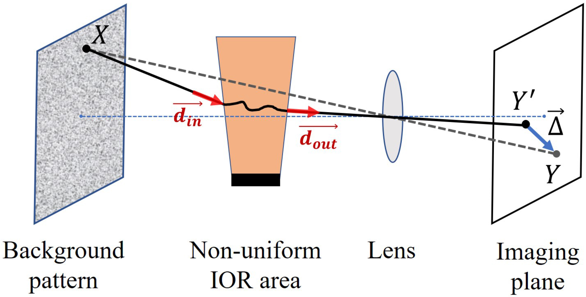
Figure 2.
Geometrical details of the (a) non–beveled nozzle, (b) double–beveled nozzle, and (c) double−beveled nozzle [40].
Figure 2.
Geometrical details of the (a) non–beveled nozzle, (b) double–beveled nozzle, and (c) double−beveled nozzle [40].

Figure 3.
A schematic for the TBOS setup.

Figure 4.
(a) Fields of displacement amplitude at selected views and (b) associated light deflections.
Figure 4.
(a) Fields of displacement amplitude at selected views and (b) associated light deflections.

Figure 5.
Comparison of between CFD data and reconstruction results: (left) the 3D spatial distribution, (center) –slice at mm, and (right) –slice at mm.
Figure 5.
Comparison of between CFD data and reconstruction results: (left) the 3D spatial distribution, (center) –slice at mm, and (right) –slice at mm.

Figure 6.
Comparison of profiles: (a,b) are sampled at ① and ② marked in Figure 5, respectively.
Figure 6.
Comparison of profiles: (a,b) are sampled at ① and ② marked in Figure 5, respectively.

Figure 7.
Comparison of between CFD and reconstruction results: (left) the 3D spatial distribution, (center) –slice at mm, and (right) –slice at mm.
Figure 7.
Comparison of between CFD and reconstruction results: (left) the 3D spatial distribution, (center) –slice at mm, and (right) –slice at mm.

Figure 8.
Comparison of profiles: (a,b) are sampled at ① and ② marked in Figure 7, respectively.
Figure 8.
Comparison of profiles: (a,b) are sampled at ① and ② marked in Figure 7, respectively.

Figure 9.
(a) Pixel displacement diagram at a certain camera viewing angle. (b) Pixel displacement diagram corresponding to the viewing angle under a 2D silhouette (white closed line segment). (c) Visual hull, the interior of which represents the flow field flow area.
Figure 9.
(a) Pixel displacement diagram at a certain camera viewing angle. (b) Pixel displacement diagram corresponding to the viewing angle under a 2D silhouette (white closed line segment). (c) Visual hull, the interior of which represents the flow field flow area.

Figure 10.
Comparison of of FDK and CGLS reconstruction results after employing VH.

Figure 11.
Comparison of profiles: (a,b) are sampled at ① and ② marked in Figure 7, respectively.
Figure 11.
Comparison of profiles: (a,b) are sampled at ① and ② marked in Figure 7, respectively.

Figure 12.
Upon incorporating the VH, a comparative analysis of the reconstruction results: (a–d) are the cases using FDK with the noise intensity ratio of 0%(no-noise), 1%, 2%, and 5% respectively, and (e–h) are the cases using CGLS under the same condition.
Figure 12.
Upon incorporating the VH, a comparative analysis of the reconstruction results: (a–d) are the cases using FDK with the noise intensity ratio of 0%(no-noise), 1%, 2%, and 5% respectively, and (e–h) are the cases using CGLS under the same condition.

Figure 13.
Cross-sectional views depicting the downstream development of jet flows from different nozzles: (top) circular nozzle, (middle) double–beveled nozzle, and (bottom) double–beveled nozzle.
Figure 13.
Cross-sectional views depicting the downstream development of jet flows from different nozzles: (top) circular nozzle, (middle) double–beveled nozzle, and (bottom) double–beveled nozzle.


Table 1.
Settings for the generation of synthetic BOS images.
| Parameter | Setting |
|---|---|
| DCB | 1500 mm |
| DCO | 750 mm |
| Reconstruction resolution | voxels |
| Measurement size | mm3 |
| Lens focal length | 50 mm |
| Pixel resolution | pixels |
| Pixel physical size | μm2 |
| resolution | |
| Camera array | Coplanar |
| Camera number | 15 |
Table 2.
Reconstruction results from different algorithms under axisymmetric and weakly non-axisymmetric conditions.
Table 2.
Reconstruction results from different algorithms under axisymmetric and weakly non-axisymmetric conditions.
| Algorithom | Axisymmetry | Non-Axisymmetry | |||||||
|---|---|---|---|---|---|---|---|---|---|
| t(s) | Peak | RMSE | t(s) | Peak Error (%) | RMSE () | ||||
| Error (%) | () | No-VH | VH | No-VH | VH | VH * | |||
| FDK | 13 | 0.3 | 1.07 | 2 | 7.1 | 7.1 | 10.89 | 3.83 | 16.67 |
| SIRT | 401 | 40 | 5.97 | 197 | 40 | – | 6.42 | – | – |
| SART | 2038 | 1.8 | 2.44 | 292 | 37 | – | 6.20 | – | – |
| CGLS | 77 | 1.9 | 2.02 | 32 | 36 | 9.3 | 6.24 | 3.67 | 5.06 |
* This case is conducted under the influence of noise pollution with an intensity ratio of 5%.
Disclaimer/Publisher’s Note: The statements, opinions and data contained in all publications are solely those of the individual author(s) and contributor(s) and not of MDPI and/or the editor(s). MDPI and/or the editor(s) disclaim responsibility for any injury to people or property resulting from any ideas, methods, instructions or products referred to in the content. |
© 2024 by the authors. Licensee MDPI, Basel, Switzerland. This article is an open access article distributed under the terms and conditions of the Creative Commons Attribution (CC BY) license (https://creativecommons.org/licenses/by/4.0/).
Share and Cite
MDPI and ACS Style
Jia, T.; Li, J.; Wu, J.; Xiong, Y. Tomographic Background-Oriented Schlieren for Axisymmetric and Weakly Non-Axisymmetric Supersonic Jets. Symmetry 2024, 16, 596. https://doi.org/10.3390/sym16050596
AMA Style
Jia T, Li J, Wu J, Xiong Y. Tomographic Background-Oriented Schlieren for Axisymmetric and Weakly Non-Axisymmetric Supersonic Jets. Symmetry. 2024; 16(5):596. https://doi.org/10.3390/sym16050596
Chicago/Turabian StyleJia, Tong, Jiawei Li, Jie Wu, and Yuan Xiong. 2024. "Tomographic Background-Oriented Schlieren for Axisymmetric and Weakly Non-Axisymmetric Supersonic Jets" Symmetry 16, no. 5: 596. https://doi.org/10.3390/sym16050596
Note that from the first issue of 2016, this journal uses article numbers instead of page numbers. See further details here.