

Interpretable Machine Learning for Geochemical Anomaly Delineation in the Yuanbo Nang District, Gansu Province, China

1
China Aero Geophysical Survey and Remote Sensing Center for Natural Resources, Beijing 100083, China
2
Department of Geology, University of the Free State, Bloemfontein 9301, South Africa
*
Authors to whom correspondence should be addressed.
Minerals 2024, 14(5), 500; https://doi.org/10.3390/min14050500
Submission received: 1 March 2024
/
Revised: 27 April 2024
/
Accepted: 3 May 2024
/
Published: 10 May 2024
(This article belongs to the Special Issue Multi-Method (Geo-) Thermochronology and Trace Elements Tracing Magmatism, Mineralization and Tectonic Evolution)
Abstract
:Machine learning (ML) has shown its effectiveness in handling multi-geoinformation. Yet, the black-box nature of ML algorithms has restricted their widespread adoption in the domain of mineral prospectivity mapping (MPM). In this paper, methods for interpreting ML model predictions are introduced to aid ML-based MPM, with the goal of extracting richer insights from the ML modeling of an exploration geochemical dataset. The partial dependence plot (PDP) and accumulated local effect (ALE) plot, along with the SHAP value analysis, were utilized to demonstrate the application of random forest (RF) modeling within both regression and classification frameworks. Initially, the random forest regression (RFR) model established the relationship between the concentrations of Au and those of elements such as As, Sb, and Hg in the study area, and from this model, the most important geochemical elements and their quantitative relationships with Au were revealed by their contributions in the modeling through PDP and ALE analyses. Secondly, the RF classification modeling established the relationships of mineralization occurrences (i.e., known mineral deposits) with geochemical elements (i.e., Au, As, Sb, Hg, Cu, Pb, Zn, and Ag), as did RFR modeling. The most important geochemical elements for indicating regional Au mineralization and the trajectories of PDP and ALE reached a consensus that As and Sb contributed the most, both in the regression and classification modeling, with regard to Au mineralization. Finally, the SHAP values illustrated the behavior of the training samples (i.e., known mineral deposits) in RF modeling, and the resulting prospectivity map was evaluated using receiver operating characteristics.
1. Introduction
The verification of anomalous metal concentrations is the foundation of geochemical exploration for mineral deposits [1], and geochemical anomalies generally result from the formation of mineral deposits or the decomposition of mineral deposits in the form of primary or secondary dispersion haloes. For the assessment of metal concentrations in a given study area through geochemical exploration, there are four general criteria proposed by [2]: (1) the magnitude of geochemical values and background; (2) the size and shape of anomalous areas; (3) geological setting; and (4) the extent to which the local environment may have influenced the metal content and the pattern of anomalies. Another criterion according to [3] is the zonality of elements in anomalies. To explore these criteria, various methods have been developed and applied, ranging from the traditional standard statistical methods to the ongoing popular machine learning (ML) methods. For example, mean ± 2 × standard deviation, probability plots [4], and histograms of frequency distributions are routine for discriminating anomalously high as well as anomalously low levels of metal concentration at early stage. Statistical analyses conducted on geochemical data often unveil linear correlations [5]. Considering the spatial structure of geochemical data, moving average [6], spatial factor analysis [7], and kriging [8] are among the popular spatial statistical methods for modeling geochemical data distribution. With regard to geochemical background, local spatial variations are common in the data, which may lead to the misclassification of weak geochemical anomalies as background. To deal with the problem of weak geochemical anomalies that are of only slightly higher concentration values compared to that of background but might be associated with mineral deposits [9], the family of fractal/multifractal models has been used widely for modeling geochemical background variation [10,11,12]. Other popular methods for dealing with geochemical background variation include trend surface analysis [13] and geographically weighted regression [14]. While these techniques have proven effective in identifying weak geochemical anomalies, their assumptions about data distribution (e.g., regularly and densely distributed sampling points) make them unable to depict the complexity of geochemical background variation perfectly.
Machine learning algorithms are well suited for quantifying intricate and nonlinear geochemical data, enabling the circumvention of traditional multivariate statistical methods that rely on data conforming to a predetermined multivariate probability distribution hypothesis [15]. When labeled samples are limited, unsupervised machine learning, particularly the autoencoder network and its variations, has demonstrated effectiveness in detecting geochemical anomalies [16]. The availability of sufficient labeled samples representing geochemical anomaly classes (i.e., associated with known mineral deposits) and geochemical background classes empowers exploration geochemists to establish a supervised machine learning pattern recognition framework for detecting geochemical anomalies [17]. The state-of-the-art supervised ML algorithms have the potential for the detection of geochemical anomalies. For example, the support vector machine (SVM) and its natural extension one-class support vector machine (OCSVM) have been introduced to explore geochemical anomalies in complex geological settings [17,18].
Despite machine learning, particularly its subset deep learning (e.g., convolutional neural networks), showcasing remarkable performance in specific research fields, the increasing model complexity and the utility of black-box models make it a challenge to understand data processing in certain ML algorithms [19]. This paper focuses on methods that address the interpretability of machine learning predictions regarding geochemical anomalies, aiding exploration geochemists in comprehending them for mineral exploration purposes. To this end, the partial dependence plot (PDP) and the accumulated local effect (ALE) plot were applied to assist exploration through geochemical data analysis in the framework of regression and classification by ML modeling. Moreover, the SHAP value analysis was adopted to help understand the contribution of known mineral deposits as training samples in the random forest (RF) classification modeling of geochemical data.
2. Material and Methods
2.1. Study Area
The study area of Yuanbo Nang District is in Xiahe County, Gansu Province, China. It belongs to the western sector of Qinling Orogen, which is endowed with huge potential for different mineral deposits [20]. The primary rock types in the study area are represented by the Daheba Formation and Jiangligou Formation, and the primary distinctions among the constituents of these two formations are found in the composition of the rocks, their cyclical arrangements, and variations in grain size. For instance, the 1st member of the Jiangligou Formation predominantly comprises medium-to-fine-grained plagioclase-quartz sandstone, fine-grained plagioclase sandstone, fine-grained plagioclase lithic sandstone, medium-to-fine-grained plagioclase quartz lithic sandstone, and siltstone. In contrast, the 1st member of the Daheba Formation is mainly characterized by medium-to-coarse-grained plagioclase quartz sandstone, medium-to-fine-grained plagioclase lithic sandstone, and coarse-grained quartz arenite, exhibiting rhythmic cyclic superposition. Additionally, within the same formation, there are differences in color and grain size. In the southeast sector of the study area, Neogene Formation occurs with mainly sandy conglomerate. The Quaternary sediments distributed across the study area comprise sand, gravel, clay, and humus. The predominant structures in the study area consist of NE-trending faults, with a limited number of inferred faults oriented in the SE direction. Among the 12 mineral deposits in the study area, 10 of them exhibit Au mineralization while the remaining 2 display Sb mineralization. All of these deposits belong to the medium-to-low-temperature type of magmatic-hydrothermal deposits [21] (Figure 1).
The geochemical dataset utilized in this study includes 1859 stream sediment samples, which were collected at a scale of 1:50,000 by the Third Institute of Geology and Mineral Exploration, Gansu Provincial Bureau of Geology and Mineral Exploration and Development. Inductively coupled plasma–mass spectrometry was employed to analyze the samples for 16 elements (i.e., Au, As, Sb, Hg, Co, Cr, Cu, Ni, Pb, Zn, Sn, Ag, Mo, Cd, W, and Bi). Among these samples, eight elements (i.e., Au, As, Sb, Hg, Cu, Pb, Zn, and Ag) were identified as potentially linked to gold (Au) and antimony (Sb) mineralization within the region. These elements were chosen for the purpose of detecting geochemical anomalies.
2.2. Random Forest
RF has raised much interest in the field of mineral prospectivity mapping (MPM) because its results are easy to understand, it needs a few parameters to be set, and its processing speed during training is satisfactory [22]. As an ensemble learning method, RF comprises a collection of decision trees [23]. CART (classification and regression trees), proposed by [24], forms the basis of the RF method. With a training dataset, an ensemble of decision trees can be built, and prediction results can be obtained using the mode of predictions (in a classification framework) or the mean of predictions (in a regression framework) by individual trees [25]. In the process of constructing an RF model, independent trees are built by the unique bootstrap sampling of the training dataset, whereby the bootstrap sampling function randomly divides the training dataset into homogenous subsets. Then, the random subsets of samples are utilized for growing and training every tree, and the remaining subset (i.e., out-of-bag (OOB) samples) are used for validation and assessment of model accuracy [25,26]. An important feature of RF is its capacity to assess the relative importance of the input variables by building alternating decision trees including and excluding every variable in the calculation of mean-square error (MSE) and node purity. The estimation of the relative importance of a variable is performed by assessing the increment of the prediction error when OOB data for that variable are permutated, while all the other variables are left unchanged [23]. In this study, RF modeling for the delineation of geochemical anomalies was performed in both the regression and classification frameworks.
2.3. Partial Dependence Plot (PDP)
The PDP depicts changes in average predicted values as specified feature(s) vary over their marginal distribution [27]. It has made a great contribution to the understanding of various supervised ML applications across a variety of disciplines. A PDP can demonstrate the relationship (e.g., linear, monotonic, or complex) between a target variable and predictor variables. Let and let be the complement set of . Then, the PDP for regression is defined as follows:
where and are subsets of predictors; denotes the features for which PDPs are made; and represents the complement features used in the ML model ; and comprise the total feature space. The PDP marginalizes the outcome of ML modeling over the distribution of a feature in a set of . Thus, the function depicts the relationship between the features in and the predictions.
In practice, the estimation of is performed by calculating averages in the training data via the Monte Carlo method; thus,
where represents the different values of observed in the training data, and denotes the number of instances in the dataset. This equation yields the average marginal effect on the prediction for a given value of . However, the PDP assumes that the features in are not correlated with the features in . The violation of this assumption may lead to very unlikely or impossible data points in the PDP. In the context of classification, where the ML model outputs probabilities, the PDP shows the probability for a certain class given different values for a feature in [27].
2.4. Accumulated Local Effect (ALE) Plot
An ALE plot, like PDP, describes the average influence of features on the prediction by an ML model. However, it is deemed to be a faster and more unbiased approach than the PDP. Using either a PDP or an ALE plot, a complex prediction function can be reduced to a function that depends only on one (or two) features by averaging the influence of the other features. However, the PDP averages the prediction over the marginal distribution. In contrast, rather than averaging the prediction directly, the ALE plot calculates the differences in prediction conditioned on a feature in , and it integrates the derivative over the feature in S for estimating the effect; thus,
The formula for ALE indicates that it averages the differences in predictions, not the prediction itself, so it is a gradient. In practice, the differences in predictions are replaced by the differences in prediction over an interval (Figure 2).
2.5. SHAP Analysis
The SHAP analysis, proposed by [28] is a popular method for characterizing the performance of an ML model based on the game theory [29] and local explanations [30]. It was originally proposed as an axiomatic description of a fair distribution of a total surplus for all players, which can be used in predictive models in which every variable resembles a player.
Let us take a coalition game as a tuple where represents a finite set of players and serves as a characteristic function with , defined over (i.e., subsets of ) that characterizes the payoff of each subset of N. The purpose of these definitions in such a coalition game is to obtain a solution for allocating the total amount of payoff to players, i.e., to every player. Here, denotes the allotted payoff to player in terms of characteristic function . Thus, a Shapley value represents a distribution solution with unique properties [31].
For a game , the Shapley value of a player is defined as follows:
Thus, the Shapley value of player is the weighted sum of the contribution of in each subset of . The contribution of to a subset is defined by .
Although the Shapley value has been originally formulated in the context of the game theory with straightforward mathematical definition, it has been recently utilized for explaining complex models generated by ML algorithms, but the connotation of taking it as a tool for model interpretation has not been illustrated yet [31].
3. Results and Discussion
Since eight elements (Au, As, Sb, Hg, Cu, Pb, Zn, and Ag) were analyzed in this study (Figure 3), the parameters for the number of trees (k) and the number of features (m) randomly sampled at each split were set as k = 1000 and m = 3 after a trial-and-error process. Both k and m settings were utilized for regression and classification in RF modeling.
3.1. Regression by RF Modeling
The regression analysis in this study aims to find associations between known mineralization and potentially relevant geochemical elements. As the study area is dominated by Au mineralization, Au served as the dependent variable, and the other seven elements served as independent variables, forming the inputs to random forest regression (RFR) modeling. Based on the ranks of variable importance, As and Sb were found to be the most significant contributors to the RFR in terms of MES increments and node purity (measured by the Gini index). This suggests that As and Sb are closely linked to the distribution of Au (Table 1). Further information can be provided by the ALE plot and PDP, as these plots can assist in describing the effects of features on the prediction by an ML model. The most important geochemical elements, As and Sb, had positive relationships with Au, and they exhibited similar trajectories (Figure 4 and Figure 5). For the PDP, the greatest issue is the assumption of independence, namely, that the features for calculating the PDP should not be correlated with other features. However, the ALE plot calculates the differences in predictions, and it isolates the effects of the features of interest, thereby blocking the effect of other features. Thus, overall, the trajectories of all geochemical elements in the PDP were consistent with those in the ALE plot, proving the robustness of the PDP and ALE plot in this case study.
Moreover, the ALE plots were centered with the average effect over the prediction equal to 0 by subtracting a constant. The value of the ALE can be interpreted as the main effect of the feature at a certain value compared to the average prediction of data. An ALE estimate of positive value (e.g., 0.3) means the prediction of Au is higher by 0.3 than the average prediction. Therefore, they provide potential thresholds for delineating geochemical anomalies (e.g., variable values in an ALE plot when Au = 0). As the geochemical variables As and Sb were found to be the most important variables in the RFR modeling, the thresholds of 42 for As and 9 for Sb (i.e., thresholds of ALE of Au = 0) were selected from the respective ALE plots (Figure 5) and used for geochemical anomaly delineation (Figure 6). The geochemical anomalies of As delineated 12 of the 13 known mineralized locations in the study area, and they showed a northwest trend. In contrast, the geochemical anomalies of Sb delineated fewer of the 13 known mineralized locations, but their consistent northwest trend implies 3 similar prospective areas for further exploration (Figure 6). Moreover, in the scenario of MPM using supervised learning, the selection of negative samples (e.g., non-deposits) for supervised MPM remains a challenge [32,33]. Here, areas excluding As and Sb anomalies provide preferred locations for creating negative samples. Thus, in this study, the 13 known mineralized locations were utilized as positive samples, and areas excluding As and Sb anomalies (i.e., areas with Sb values of >9 and As values of >42) were outlined and used as areas for the selection of randomly negative samples (13 non-deposits) for the subsequent RF classification modeling (Figure 6).
3.2. Classification by RF Modeling
The RFR modeling provided insights into the relationships of As, Sb, Hg, Cu, Pb, Zn, and Ag with the target Au mineralization in the study area. However, there are scenarios where mineralization is absent in the case of false anomalies with high magnitude [34]. For example, areas with high values of Au may not mean favorability of an area for Au mineralization. It is necessary to discover the correlation of geochemical elements with known mineralized locations. RF classification was applied to correlate the known mineralization areas and the concentrations of the studied geochemical elements (i.e., Au, As, Sb, Hg, Cu, Pb, Zn, and Ag).
In the RF modeling, the importance of evidential maps was evaluated by the mean decrease in accuracy and the mean decrease in Gini indices. The former is calculated from OOB data and indicates the reduction in accuracy across the entire RF modeling, while the latter measures the average increase in purity achieved by utilizing splits of a particular variable.
The results of RF modeling indicate that As and Sb are the most important geochemical elements, which is consistent with the results of RFR modeling (Figure 7). Au ranked fourth behind As, Sb, and Ag. In contrast to the PDP and the ALE plot, in RFR modeling, Au, As, Ag, and Sb not only demonstrated similar trajectories in the PDP and the ALE plot (Figure 8 and Figure 9) but also showed significant differences to the other geochemical variables (i.e., Hg, Cu, Pb, and Zn). Geological/geochemical processes can be recognized by a continuous range of variable responses and the corresponding relative increase or decrease in element concentration, and high-density surveys are capable of detecting local scale processes [5]. The behaviors of the geochemical variables in RF modeling and the spatial distributions of their concentrations (Figure 3) imply that Au, As, Ag, and Sb had a positive influence on the formation of known mineralization. The coincidence of the locations of known mineralization with smaller and less intense anomalies may be more indicative of the occurrence of mineral deposits [1]. This prompts the introduction of interpretable ML for geochemical anomaly detection.
Besides the PDP and the ALE plot, which shed light on the relationships between the geochemical elements of interest and known mineralization (i.e., Au element concentration in RFR modeling and Au deposits in RF modeling), the Shapley values were adopted to illustrate the behavior of the training samples in ML-based prediction. In the context of RF modeling for MPM and given the current set of geochemical variables, the Shapley value serves as an approximation of how much a particular value of a geochemical variable contributes to the disparity between the actual prediction and the average prediction.
Figure 10 shows the contributions of each feature of an instance (i.e., training sample) in RF modeling toward known mineralization. Figure 10a,b depict two of the negative training samples (i.e., non-deposits), whereas Figure 10c,d depict the training samples taken from locations of known mineralization. Both the negative and positive training samples imply that As, Sb, and Ag contributed the most. This aligns with the importance of the variable in terms of accuracy and the Gini index (Figure 7). Moreover, the geochemical variables of negative training samples showed a negative contribution, in contrast to that of the positive training samples, and the Shapley values of the positive samples varied, with As (labeled 5), Sb (labeled 12) and Ag (labeled 4, 5, 6, and 8) having negative contributions (Figure 11 and Figure 12). These findings suggest that the Shapley value holds promise as a tool for evaluating the efficacy of a training dataset in machine learning-based mineral prospectivity mapping (MPM), particularly in the context of identifying non-deposit locations for use as negative training samples.
The final prospectivity map shows that areas of high potential delineated most of the known mineral deposits (Figure 12). The performance of random forest (RF) modeling was assessed using the receiver operating characteristic (ROC) curve, which illustrates the true-positive rate versus the false-positive rate, with the area under the curve (AUC) indicating the overall performance of the RF modeling [35]. By utilizing the probability of mineralization occurrence to compute the AUC, we obtained a value of 0.917 for deposits (i.e., positive training samples) and 0.182 for non-deposits. These results suggest that RF modeling effectively distinguished between known mineral deposit locations and the selected non-deposit locations (Figure 13). The relationship between the distribution of prospectivity values obtained and the known mineral deposits was evaluated using prediction–area (P-A) plots and concentration–area (C-A) fractal analysis. The P-A plot illustrates the ratio of the area covered by prospectivity classes (relative to the total study area) against the ratio of known mineral occurrences (relative to the total number of known occurrences) predicted by those respective prospectivity classes [36]. The results indicate that RF modeling identified 9.7% of the study area, accurately capturing 84.6% of the known mineral deposits. In contrast, the C-A fractal analysis identified three probability categories: high potential (probability > 0.80), moderate potential (0.22 < probability < 0.80), and low potential (probability < 0.22) (Figure 14).
4. Conclusions
Machine learning algorithms have demonstrated their effectiveness in mineral prospectivity mapping (MPM). Nonetheless, the black-box nature of the majority of ML algorithms results in limited insights into the relationship between input variables (i.e., evidence maps) and the target variable (i.e., mineral deposits). In this study, PDP and ALE plot analyses were utilized to visualize the impacts of geochemical variables on documented mineralization within the context of regression and classification models. Additionally, SHAP analysis was employed to elucidate the performance of individual training samples in machine learning modeling. The utilization of these interpretive tools effectively yielded quantitative insights from the concentrations of geochemical elements for delineating geochemical anomalies. These tools enhanced the credibility of derived geochemical anomaly information, suggesting that research on interpretable machine learning-based predictions can further advance the practice of mineral prospectivity mapping (MPM).
The work discussed here involved a combination of mathematical concepts with the identification of geochemical anomalies, that is, the transformation of mathematical parameters into geochemical parameters to improve the recognition and assessment of geochemical anomalies. Nevertheless, in the study area, the interpretation of geochemical anomalies using the proposed methodology can probably be enriched by additional analyses, e.g., combined petrographic and ore microscopic analyses of known mineralization, as these would provide a more holistic understanding of the geological processes at play and reveal further insights into the mineralogical composition and microstructural features of the studied area. However, this is a recommendation for further study.
Author Contributions
Conceptualization, S.Z.; writing—original draft preparation, S.Z. and E.J.M.C.; writing—review and editing, E.J.M.C.; supervision, C.F.; visualization, X.Q.; project administration, W.Z.; funding acquisition, C.F. All authors have read and agreed to the published version of the manuscript.
Funding
This research was funded by the China Geological Survey Project (Grant no. DD20191011).
Data Availability Statement
Data available on request due to restrictions.
Acknowledgments
We thank the anonymous reviewers for their constructive comments.
Conflicts of Interest
Shuai Zhang is an employee of China Aero Geophysical Survey and Remote Sensing Center for Natural Resources. The paper reflects the views of the scientists and not the institution.
References
- Goldberg, I.S.; Abramson, G.Y.; Los, V.L. Exploration Criteria for Appraising Geochemical Anomalies through Mapping Geochemical Systems. Geochem. Case Hist. Geochmical Explor. Methods 2007, 963–968. [Google Scholar]
- Rose, A.W.; Hawkes, H.E.; Webb, J.S. Geochemistry in Mineral Exploration, 2nd ed.; Academic Press: London, UK, 1979; p. 657. [Google Scholar]
- Grigoryan, S. Primary geochemical halos in prospecting and exploration of hydrothermal deposits. Int. Geol. Rev. 1974, 16, 12–25. [Google Scholar] [CrossRef]
- Reimann, C.; Filzmoser, P.; Garrett, R.G. Background and threshold: Critical comparison of methods of determination. Sci. Total Environ. 2005, 346, 1–16. [Google Scholar] [CrossRef]
- Grunsky, E.C.; Grunsky, E.C.; Caritat, P.D.; Caritat, P.D. State-of-the-art analysis of geochemical data for mineral exploration. Geochem. Explor. Environ. Anal. 2019, 20, 217–232. [Google Scholar] [CrossRef]
- Cheng, Q.; Agterberg, F.P.; Bonham-Carter, G.F. A spatial analysis method for geochemical anomaly separation. J. Geochem. Explor. 1996, 56, 183–195. [Google Scholar] [CrossRef]
- Grunsky, E.C.; Agterberg, F.P. Spatial and multivariate analysis of geochemical data from metavolcanic rocks in the Ben Nevis area, Ontario. Math. Geol. 1988, 20, 825–861. [Google Scholar] [CrossRef]
- Jimenez-Espinosa, R.; Sousa, A.J.; Chica-Olmo, M. Identification of geochemical anomalies using principal component analysis and factorial kriging analysis. J. Geochem. Explor. 1993, 46, 245–256. [Google Scholar] [CrossRef]
- Zuo, R.; Carranza, E.J.M.; Wang, J. Spatial analysis and visualization of exploration geochemical data. Earth-Sci. Rev. 2016, 158, 9–18. [Google Scholar] [CrossRef]
- Zuo, R.; Wang, J. Fractal/multifractal modeling of geochemical data: A review. J. Geochem. Explor. 2016, 164, 33–41. [Google Scholar] [CrossRef]
- Cheng, Q.; Agterberg, F.; Ballantyne, S. The separation of geochemical anomalies from background by fractal methods. J. Geochem. Explor. 1994, 51, 109–130. [Google Scholar] [CrossRef]
- Ford, A.; Blenkinsop, T.G. Combining fractal analysis of mineral deposit clustering with weights of evidence to evaluate patterns of mineralization: Application to copper deposits of the Mount Isa Inlier, NW Queensland, Australia. Ore Geol. Rev. 2008, 33, 435–450. [Google Scholar] [CrossRef]
- Wang, H.; Zuo, R. A comparative study of trend surface analysis and spectrum–area multifractal model to identify geochemical anomalies. J. Geochem. Explor. 2015, 155, 84–90. [Google Scholar] [CrossRef]
- Tian, M.; Wang, X.; Nie, L.; Zhang, C. Recognition of geochemical anomalies based on geographically weighted regression: A case study across the boundary areas of China and Mongolia. J. Geochem. Explor. 2018, 190, 381–389. [Google Scholar] [CrossRef]
- Yin, B.; Zuo, R.; Xiong, Y.; Li, Y.-S.; Yang, W. Knowledge discovery of geochemical patterns from a data-driven perspective. J. Geochem. Explor. 2021, 231, 106872. [Google Scholar] [CrossRef]
- Zhang, S.; Xiao, K.; Carranza, E.J.M.; Yang, F.; Zhao, Z. Integration of auto-encoder network with density-based spatial clustering for geochemical anomaly detection for mineral exploration. Comput. Geosci. 2019, 130, 43–56. [Google Scholar] [CrossRef]
- Gonbadi, A.M.; Tabatabaei, S.H.; Carranza, E.J.M. Supervised geochemical anomaly detection by pattern recognition. J. Geochem. Explor. 2015, 157, 81–91. [Google Scholar] [CrossRef]
- Chen, Y.; Wu, W. Application of one-class support vector machine to quickly identify multivariate anomalies from geochemical exploration data. Geochem. Explor. Environ. Anal. 2017, 17, 231–238. [Google Scholar] [CrossRef]
- Saeed, W.; Omlin, C.W.P. Explainable AI (XAI): A Systematic Meta-Survey of Current Challenges and Future Opportunities. arXiv 2021, arXiv:abs/2111.06420. [Google Scholar] [CrossRef]
- Mao, J.; Qiu, Y.; Goldfarb, R.J.; Zhang, Z.; Garwin, S.L.; Fengshou, R. Geology, distribution, and classification of gold deposits in the western Qinling belt, central China. Miner. Depos. 2002, 37, 352–377. [Google Scholar] [CrossRef]
- Shi, Y.X.; Li, K.N.; Shi, H.L.; Jin, D.G.; Liang, Z.L. Report on the prospect survey of gold mines in Xiahe-Hezuo district; Third Institute Geological and Mineral Exploration of Gansu Provincial Bureau of Geology and Mineral Resources: Gansu, China, 2017; p. 155. (In Chinese) [Google Scholar]
- Wang, J.; Zuo, R.; Xiong, Y. Mapping mineral prospectivity via semi-supervised random forest. Nat. Resour. Res. 2019, 29, 189–202. [Google Scholar] [CrossRef]
- Breiman, L. Random forests. Mach. Learn. 2001, 45, 5–32. [Google Scholar] [CrossRef]
- Breiman, L.; Friedman, J.; Olshen, R.A.; Stone, C.J. Classification and Regression Trees; Chapman & Hall: New York, NY, USA, 1984. [Google Scholar]
- Rasaei, Z.; Bogaert, P. Spatial filtering and Bayesian data fusion for mapping soil properties: A case study combining legacy and remotely sensed data in Iran. Geoderma 2019, 344, 50–62. [Google Scholar] [CrossRef]
- Khanal, S.K.; Fulton, J.P.; Klopfenstein, A.; Douridas, N.; Shearer, S.A. Integration of high resolution remotely sensed data and machine learning techniques for spatial prediction of soil properties and corn yield. Comput. Electron. Agric. 2018, 153, 213–225. [Google Scholar] [CrossRef]
- Molnar, C. Interpretable Machine Learning: A Guide for Making Black Box Models Explainable; Lulu.com.: Morrisville, NC, USA, 2019; Available online: https://www.bookstack.cn/read/interpretable-ml-book/8935d4eb447a2642.md (accessed on 2 February 2024).
- Lundberg, S.M.; Lee, S.-I. A Unified Approach to Interpreting Model Predictions. arXiv 2017, arXiv:abs/1705.07874. [Google Scholar]
- Shapley, L. A value for n-person games. In The Shapley Value: Essays in Honor of Lloyd, S. Shapley; Roth, A., Ed.; Cambridge University Press: Cambridge, UK, 1988; pp. 31–40. [Google Scholar] [CrossRef]
- Ribeiro, M.T.; Singh, S.; Guestrin, C. Why Should I Trust You? Explaining the Predictions of Any Classifier. In Proceedings of the 22nd ACM SIGKDD International Conference on Knowledge Discovery and Data Mining, San Francisco, CA, USA, 13–17 August 2016; Association for Computing Machinery: New York, NY, USA, 2016; pp. 1135–1144. [Google Scholar]
- Ma, S.; Tourani, R. Predictive and Causal Implications of using Shapley Value for Model Interpretation. J. Mach. Learn. Res. 2020, arXiv:2008.05052. [Google Scholar]
- Carranza, E.J.M.; Laborte, A.G. Data-Driven Predictive Modeling of Mineral Prospectivity Using Random Forests: A Case Study in Catanduanes Island (Philippines). Nat. Resour. Res. 2015, 25, 35–50. [Google Scholar] [CrossRef]
- Zuo, R.; Wang, Z. Effects of Random Negative Training Samples on Mineral Prospectivity Mapping. Nat. Resour. Res. 2020, 29, 3443–3455. [Google Scholar] [CrossRef]
- Levinson, A.A. Introduction to Exploration Geochemistry; Applied Publishing Ltd.: Calgary, AB, Canada, 1974; p. 611. [Google Scholar]
- Zhang, S.; Xiao, K.; Carranza, E.J.M.; Yang, F. Maximum Entropy and Random Forest Modeling of Mineral Potential: Analysis of Gold Prospectivity in the Hezuo–Meiwu District, West Qinling Orogen, China. Nat. Resour. Res. 2018, 28, 645–664. [Google Scholar] [CrossRef]
- Yousefi, M.; Carranza, E.J.M. Prediction–area (P–A) plot and C–A fractal analysis to classify and evaluate evidential maps for mineral prospectivity modeling. Comput. Geosci. 2015, 79, 69–81. [Google Scholar] [CrossRef]
Figure 1.
Simplified geological and mineral map of the study area.

Figure 2.
Schematic example of ALE calculation for feature X1 (correlated with X2). First, X1 is divided into intervals (dotted vertical lines). For the data points within an interval, the differences in the prediction when X1 is replaced with the upper and lower limits of the interval (solid horizontal lines) are calculated, accumulated, and centered, yielding the ALE curve (modified from [23]).

Figure 3.
Geochemical elements used in RF modeling.

Figure 4.
Partial dependence plot of geochemical element for RFR modeling.

Figure 5.
ALE of geochemical element for RFR modeling.

Figure 6.
Non-deposit area selection based on ALE plots of As and Sb.

Figure 7.
The relative importance of geochemical variables used in RF modeling.

Figure 8.
Partial dependence plot of geochemical elements used in RF modeling.

Figure 9.
ALE plots of geochemical elements used in RF modeling.
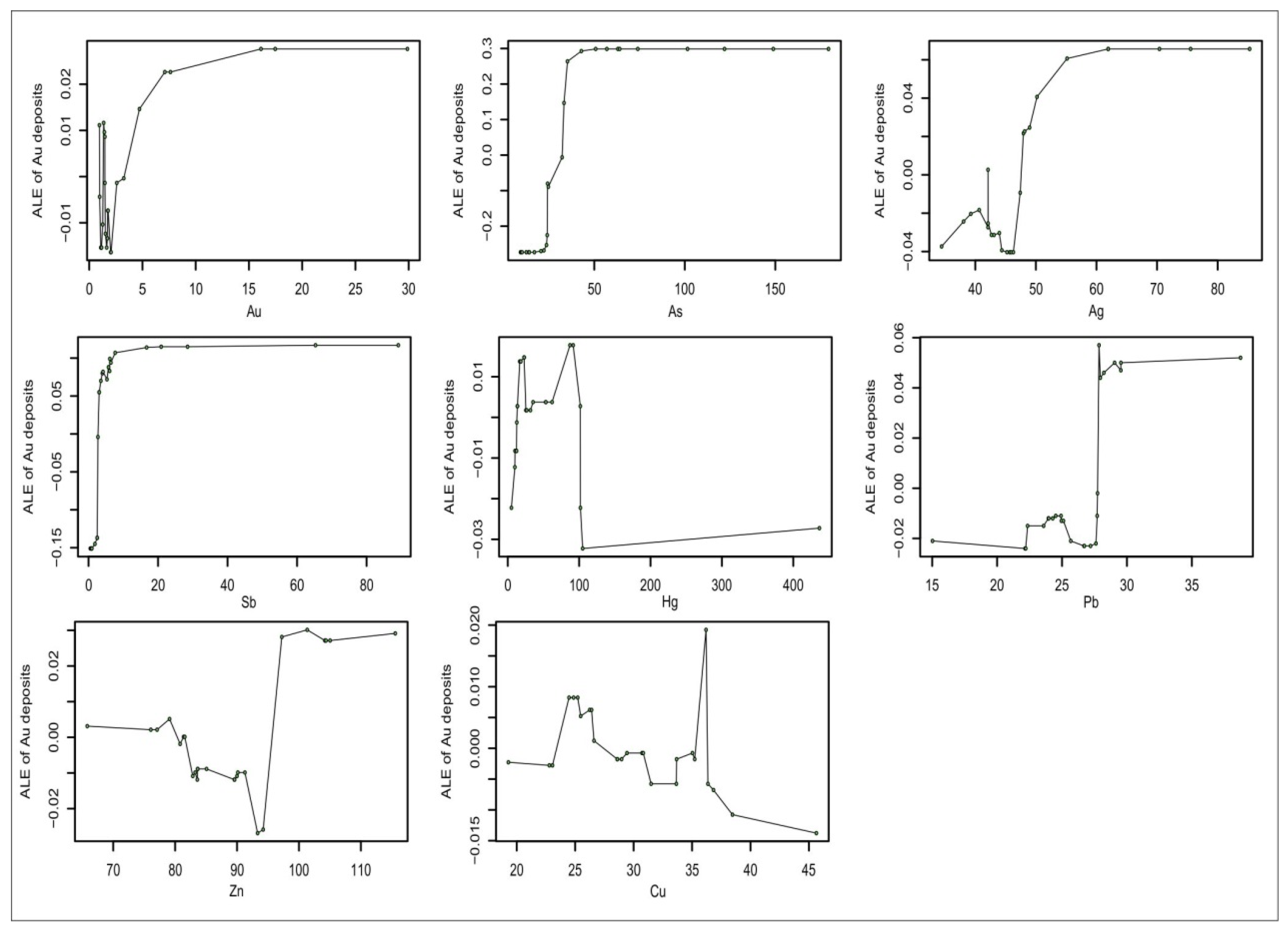
Figure 10.
Examples of Shapley value of training samples ((a,b): negative samples; (c,d): positive sample) in RF modeling toward known mineralization.
Figure 10.
Examples of Shapley value of training samples ((a,b): negative samples; (c,d): positive sample) in RF modeling toward known mineralization.

Figure 11.
Shapley values of positive training samples for known mineral deposits in RF modeling.

Figure 12.
Ternary class gold prospectivity map obtained from RF modeling.

Figure 13.
ROC curves for (a) deposits (AUC = 0.917) and (b) non-deposits (AUC = 0.182).

Figure 14.
P-A and C-A plots for gold prospectivity map.


Table 1.
Variable importance for RFR regression.
| Variables | As | Sb | Hg | Cu | Pb | Zn | Ag |
|---|---|---|---|---|---|---|---|
| %IncMSE | 5.13 | 3.61 | 0.94 | 1.54 | 0.37 | 1.91 | 0.02 |
| IncNodePurity | 2914 | 1590 | 1381 | 1269 | 1206 | 1124 | 1134 |
Disclaimer/Publisher’s Note: The statements, opinions and data contained in all publications are solely those of the individual author(s) and contributor(s) and not of MDPI and/or the editor(s). MDPI and/or the editor(s) disclaim responsibility for any injury to people or property resulting from any ideas, methods, instructions or products referred to in the content. |
© 2024 by the authors. Licensee MDPI, Basel, Switzerland. This article is an open access article distributed under the terms and conditions of the Creative Commons Attribution (CC BY) license (https://creativecommons.org/licenses/by/4.0/).
Share and Cite
MDPI and ACS Style
Zhang, S.; Carranza, E.J.M.; Fu, C.; Zhang, W.; Qin, X. Interpretable Machine Learning for Geochemical Anomaly Delineation in the Yuanbo Nang District, Gansu Province, China. Minerals 2024, 14, 500. https://doi.org/10.3390/min14050500
AMA Style
Zhang S, Carranza EJM, Fu C, Zhang W, Qin X. Interpretable Machine Learning for Geochemical Anomaly Delineation in the Yuanbo Nang District, Gansu Province, China. Minerals. 2024; 14(5):500. https://doi.org/10.3390/min14050500
Chicago/Turabian StyleZhang, Shuai, Emmanuel John M. Carranza, Changliang Fu, Wenzhi Zhang, and Xiang Qin. 2024. "Interpretable Machine Learning for Geochemical Anomaly Delineation in the Yuanbo Nang District, Gansu Province, China" Minerals 14, no. 5: 500. https://doi.org/10.3390/min14050500
Note that from the first issue of 2016, this journal uses article numbers instead of page numbers. See further details here.