Article

A Modified Enthalpic Lattice Boltzmann Method for Simulating Conjugate Heat Transfer Problems in Non-Homogeneous Media

by
Vinicius Akyo Matsuda
1,
Ivan Talão Martins
1,
Debora Carneiro Moreira
1,
Luben Cabezas-Gómez
1 and
Enio Pedone Bandarra Filho
2,*
1
Heat Transfer Research Group, Department of Mechanical Engineering, São Carlos School of Engineering (EESC), University of São Paulo (USP), São Carlos 13566-590, São Paulo, Brazil
2
Faculty of Mechanical Engineering, Federal University of Uberlândia (UFU), Av. João Naves de Ávila, 2121 Santa Monica, Uberlândia 38400-902, Minas Gerais, Brazil
*
Author to whom correspondence should be addressed.
Inventions 2024, 9(3), 57; https://doi.org/10.3390/inventions9030057
Submission received: 5 April 2024 / Revised: 9 May 2024 / Accepted: 11 May 2024 / Published: 13 May 2024
(This article belongs to the Special Issue Innovations in Heat Exchangers)

Abstract

:
In this study, we introduced modifications to a prior existing enthalpic lattice Boltzmann method (LBM) tailored for simulating the conjugate heat transfer phenomena in non-homogeneous media with time-dependent thermal properties. Our approach is based upon the incorporation of the remaining terms of a conservative energy equation, excluding only the terms regarding flow compressibility and viscous dissipation, thereby accounting for the local and transient variations in the thermophysical properties. The solutions of verification tests, comprising assessments of both transient and steady-state solutions, validated the accuracy of the proposed model, further bolstering its reliability for analyzing heat transfer processes. The modified model was then used to perform an analysis on structured cavities under free convection, revealing compelling insights, particularly regarding transient regimes, demonstrating that the structured cavities exhibit a beneficial impact on enhancing the heat transfer processes, hence providing insights for potential design enhancements in heat exchangers. These results demonstrate the potential of our modified enthalpic LBM approach for simulating complex heat transfer phenomena in non-homogeneous media and structured geometries, offering valuable results for heat exchanger engineering and optimization.

1. Introduction

Natural convection processes have demonstrated numerous applications in refrigerating electronic devices and technology, including the cooling of printed circuit boards, memory devices, processors, and more [1,2]. This heat transfer phenomenon has also been utilized in the cooling mechanisms for buildings, electric motors, air conditioning and refrigeration systems, nuclear reactors, among others [3,4]. Typically, in these applications, the cooling process by natural convection is facilitated through heat exchangers, which come in various geometrical configurations and types. Given its widespread use and low operational cost, enhancing this heat transfer mechanism is of significant interest.
Various methods employed for this purpose involve surface modifications, such as adding fins or utilizing small cavities or grooves. Several studies found in the literature [5,6,7,8,9] investigate the impact of surface modifications on enhancing free convection heat transfer processes. Generally, these studies examine surface modifications with configurations resembling waves, employing sinusoidal functions [10,11] or evenly spaced geometries like triangular [8,12] or square [9,13] patterns. These works are often categorized based on the modifications made to horizontal [11,12], vertical [6,9,10], or inclined surfaces [7,13], typically employing experimental and Computational Fluid Dynamics (CFD) techniques to analyze the problem.
By its nature, the free-convection process occurs under conjugate heat transfer conditions, initially defined by [14]. Consequently, the numerical simulation of such a problem proves to be challenging, with many works resorting to directly imposing the boundary conditions at the fluid nodes [6,8]. Traditionally, computational procedures primarily rely on finite differences, finite volume, or finite element methods [15,16,17,18]. These methods typically involve creating coupling schemes at the solid–fluid interface, where Dirichlet and Neumann boundary conditions are imposed on different sides and the energy conservation equation is solved separately. Despite their applicability, implementing these methods on more complex interfaces can become challenging, particularly in ensuring the continuity at the interface.
On the other hand, the lattice Boltzmann method (LBM) is a mesoscopic simulation technique that solves the Boltzmann transport equation on a discrete lattice [19], offering advantages over the traditional methods. Specifically regarding the LBM models for conjugate heat transfer, the two most accurate LBM models are [20] the direct interface treatment, originally proposed by Li et al. [21], and the “enthalpy like” models, such as the one developed in Karani and Huber [22], Rihab et al. [23], Chen et al. [24].
In general, the models based on the direct interface treatment have good precision for any boundary position in relation to the boundary lattices. However, in the presence of structured surfaces or complicated geometries, the implementation of these interface conditions becomes considerably difficult. Alternatively, the “enthalpy-like” models work through the addition of specific source terms, tailored to correctly represent the target energy equation, thus not requiring special treatment for the interfaces. In this line, several works have been proposed [22,24,25,26,27].
Chen et al. [24] incorporated through a source term the effects of the local variation regarding the thermophysical properties. Additionally, the authors suggested the use of the forward Euler time discretization scheme to include the time dependence of the thermophysical properties. On the other hand, Hosseini et al. [25] proposed a method with an iterative scheme for dealing with the temperature-dependent heat capacity, which resorts to the use of a root-finding algorithm to correctly account for its variations. More recently, Kiani-Oshtorjani et al. [27], by working with a simplified conservative form of the energy equation and disregarding the flow compressibility, viscous dissipation, and time dependence of the thermophysical properties, introduced a new source term based on the variation in the thermal conductivity between the different media.
As observed in our literature review, several works employed the use of a simplified conservative energy equation [24,26,27], often disregarding the time dependence of the thermophysical properties, like the system capacitance ( ρ c p ). To address this issue, the authors of this paper proposed the derivation of a new source term, considering its derivation from the conservative form of the energy conservation equation [28] for a system without a volumetric heat source, written in terms of temperature, T, and constant-pressure specific heat, c P . Based on the work of Chen et al. [24], we derived a simple source term, which naturally accounts for the time and temperature dependence of the system’s thermophysical properties. It should be noted that the reference temperature employed for computing the body force by the Boussinesq approximation is also changed with time. In fact, this is the temperature employed for calculating the thermophysical properties. The proposal of these modifications is the main novelty of this paper.
The paper is structured into three main sections. The first section (Section 2) outlines the employed methodology, which includes the presentation of the momentum and thermal LBM models, as well as the derivation and integration of a source term to address the conjugate heat transfer. Following this, the second section (Section 3.1) presents the results obtained from the benchmark tests. These tests involve comparisons with analytical solutions for pure diffusion problems, both transient and stationary, as well as convection diffusion problems. Additionally, a mesh refinement study is conducted using natural convection results sourced from the existing literature. The final section (Section 3.2) examines the effects of the structural geometries on the natural convection problem. Finally, the principal conclusions drawn from the study are presented in the conclusion (Section 4).

2. Materials and Methods

In this section, the mathematical models employed for performing the simulations of this paper are presented. We consider the dimensional approach proposed by Martins et al. [29] given its ability to deal directly with real fluid properties.

2.1. Lattice Boltzmann Method for Fluid Flow

For the fluid flow modeling, the traditional LBE with the Bhatnagar–Gross–Krook (BGK) collision operator was used [30], which considers only a single relaxation time, τ . Given time and space discrete intervals Δ t and Δ x , the LBE for the fluid flow is provided by Equation (1) [31]. In this equation, f i is the density distribution function, f i e q represents the equilibrium distribution function, and S f i is the forcing term, which depends on the forcing scheme chosen. The sub-index i represents each discrete velocity direction, while c i is the particle velocity vector, according to the selected velocity scheme [32].
f i ( x + c i Δ t , t + Δ t ) f i ( x , t ) = Δ t τ f i ( x , t ) f i e q ( x , t ) + S f i ( x , t ) Δ t .
The equilibrium distribution functions for the fluid flow LBE are calculated by Equation (2) [33], where u and ρ are the macroscopic velocity and density, respectively, c s is the sound speed, and w i indicates the weights related to each velocity direction i, both depending on the velocity scheme considered.
f i e q ( x , t ) = w i ρ ( x , t ) 1 + c i · u c s 2 + ( c i · u ) 2 2 c s 4 u · u 2 c s 2 ( x , t ) .
In the simulations performed here, we used a two-dimensional approach with the D 2 Q 9 velocity scheme [32]. Thus, according to [32], the particle velocity vectors and the respective weights are provided by Equations (3) and (4), being c = Δ x / Δ t and c s = c / 3 .
c i = c ( 0 , 0 ) , i = 0 , ( 1 , 0 ) , ( 0 , 1 ) , ( 1 , 0 ) , ( 0 , 1 ) , i = 1 , . . . , 4 , ( 1 , 1 ) , ( 1 , 1 ) , ( 1 , 1 ) , ( 1 , 1 ) , i = 5 , . . . , 8 .
w i = 4 / 9 , i = 0 , 1 / 9 , i = 1 , . . . , 4 , 1 / 36 , i = 5 , . . . , 8 .
For the source term in Equation (1), the forcing scheme proposed by Guo et al. [34] was used. Then, the source term is defined by Equation (5), where F is the total specific force acting over the domain.
S f i = 1 Δ t 2 τ w i c i u c s 2 + ( c i · u ) c i c s 4 ( x , t ) · F ( x , t )
Additionally, the macroscopic fields can be obtained from the distribution functions as depicted in Equations (6) and (7), q being the number of discrete velocity directions (for example, q = 9 for the D 2 Q 9 scheme).
ρ ( x , t ) = i = 0 q 1 f i ( x , t )
ρ ( x , t ) u ( x , t ) = i = 0 q 1 f i ( x , t ) c i + Δ t 2 F ( x , t )
Through the Chapman–Enskog analysis [35], it is possible to recover the Navier–Stokes equation, Equation (8), from the LBE. This process results in a relationship between the relaxation time, τ , and the kinematic viscosity, ν , which is provided by ν = ( τ 0.5 Δ t ) c s 2 .
ρ u t + · ρ u u = p + · ν ρ u + u T + F .
Regarding boundary conditions (BC), the bounce-back (BB) rule was implemented for both static walls and fluid inlet BCs, provided by Equation (9), where i ¯ indicates the opposite direction of i, x b indicates the boundary nodes, and the variables with sub-index w stand for the values defined at the boundary. The more complexes geometries, such as the cavities for the natural convection, were also implemented using the BB rule.
f i ¯ ( x b , t + Δ t ) = f i * ( x b , t ) 2 w i ρ w c i · u w c s 2
The periodic kind of BC was simply implemented considering that the populations leaving one side are the same that enter at the opposite side of the domain. This relation can be expressed by the following expression: f i ( x b , t + Δ t ) = f i * ( x b + L c i Δ t , t ) , where L is the size of the domain pointing at the normal direction of the boundary.

2.2. Boussinesq Approach for Natural Convection

In natural convection, the local temperature variations cause small local density changes, which create mass fluxes through the domain because of the gravitational field influence. These fluxes are commonly denominated “convection currents”, which help to transfer the heat in the entire domain.
A practical way to include the effects of density fluctuations in the LB simulations is by using the Boussinesq approach. Instead of considering a temperature-dependent density, ρ ( T ) , it is assumed that the fluid remains at a mean density, ρ ¯ , measured at the reference temperature of T ¯ . Then, the thermal expansion coefficient can be expressed according to Equation (10), and the buoyancy force that is provided by Equation (11) is added to the momentum LBE (Equations (1) and (5)) for taking into consideration the density fluctuations. In this equation, g is the gravitational acceleration.
β e x p = 1 ρ ρ T 1 ρ ¯ / ρ ( x , t ) T ( x , t ) T ¯
F ( x , t ) = F b ( x , t ) = β e x p g ρ ¯ T ( x , t ) T ¯
In this paper, we are simulating transient conjugate heat transfer problems, including transient natural convection problems, which can be driven by a constant heat flux or surface temperature. For all cases, the determination of the reference temperature ( T ¯ ) becomes a challenge and a necessity. This is because, even if the fluid is initially at a uniform temperature, the local temperature values increase non-equally over time. Then, the mean temperature of the domain changes every time and it is needed to determine T ¯ for each time-step.
Consequently, in this work, all the fluid properties that are independent of the distribution functions are re-calculated for each new T ¯ value. These properties include the dynamic viscosity, specific heat capacity, conductivity, and thermal expansion coefficient. For this task, we propose to use polynomial approaches for determining the variation in these properties with the temperature. Here, these polynomials were obtained with the help of EES software [36]. Hence, the employed LBM model has the capability of dealing with local and temporal thermophysical property changes. The new T ¯ values are calculated explicitly, i.e., considering the average mean temperature of the fluid domain from the previous time step.

2.3. Lattice Boltzmann Method for Conjugate Heat-Transfer

As noted before, the main advantage of the “enthalpy-like” models is that no special treatment for the interfaces is needed due to the effects being naturally incorporated into the LBE through a source. Furthermore, for the link-wise approach [20], both methods have second-order accuracy when using the link-wise approach for the boundary nodes. Thus, in this paper, we propose a modification of the Chen et al. [24] model for accounting the temporal and local variations in the medium (solid and fluid) properties, considering conjugate heat transfer problems. The procedure for re-calculating the thermophysical properties as a function of the temperature was explained in the previous Section 2.2.
The conservative form of the energy conservation equation [28] for a system without volumetric heat source, written in terms of temperature, T, and constant-pressure specific heat, c P , for a generic system is provided by Equation (12). In this equation, the term ln V ln T D P d t stands for the energy transfer due to compressible effects, while τ : u refers to the viscous dissipation.
t ( ρ c p T ) + · ( ρ c p T u ) = k T + ln V ln T D P D t + τ : u + T D ρ c P D t
Now, the left-hand side of Equation (12) can be re-written as follows:
t ( ρ c p T ) + · ( ρ c p T u ) = ρ c P [ t T + · ( T u ) ] + T D ρ c P D t .
Substituting Equation (13) into Equation (12), blue we have
ρ c P [ t T + · ( T u ) ] = k T + ln V ln T D P D t + τ : u
Neglecting the viscous heat dissipation, the energy conservation equation is provided by Equation (15). It is important to note that this equation is generic enough to be valid for a non-homogeneous domain.
ρ c P [ t T + · ( T u ) ] = k T
Similarly to the model developed by Chen et al. [24], a new variable h 0 = ρ c P 0 T is defined, ρ c P 0 being a constant reference heat capacitance. Substituting T = h 0 / ρ c P 0 into Equation (15) and defining σ = ρ c p / ρ c P 0 , we obtain Equation (16), where α = k / ( ρ c p ) is the local thermal diffusivity.
t h 0 + · ( u h 0 ) = ( α h 0 ) k ρ c P 0 h 0 1 σ
Defining a new distribution function g i related to h 0 , and using the source term proposed by Seta [37], the LBE with the dimensional approach for the energy conservation equation is described by Equation (17). In this equation, Ω g i ( x , t ) is the collision operator. Considering the traditional BGK approach, it is defined as Ω i B G K = g i g i e q / τ T . Also, g i e q is the equilibrium distribution function, provided by Equation (18).
g i ( x + c i Δ t , t + Δ t ) g i ( x , t ) = Ω i ( x , t ) Δ t + Δ t w i 1 Δ t 2 τ T S g ( x , t )
g i e q = w i h 0 ( x , t ) 1 + c i · u c s 2 + ( c i · u ) 2 2 c s 4 u · u 2 c s 2 ( x , t )
By Chapman–Enskog analysis, it is possible to recover Equation (16) from the thermal LBE (Equation (17)), resulting that the relaxation time for the BGK collision operator is related to the thermal diffusivity of the domain as α = k / ( ρ c p ) by the following expression: α = ( τ T 0.5 Δ t ) c s 2 . The procedure for this analysis is provided in Appendix A. Additionally, it is possible to note that, by this expansion, the LBE only recovers the the first term on the right-hand side of Equation (16). Consequently, the other terms must be included in the LBE via the source term, which is defined by Equation (19).
S g ( x , t ) = k ρ c P 0 h 0 1 σ
The additional terms that must be added via source term to the LBE are not easy to calculate as it involves gradient of quantities depending on the distribution functions g i . Thus, it is interesting to conduct some manipulations using the definition of heat flux from Karani and Huber [22], resulting in the following representation:
k ( ρ c p ) 0 h 0 = σ k ρ c p h 0 = σ 1 Δ t 2 τ T i g i g i e q c i .
Also, the spatial derivative of 1 / σ can be evaluated by an isotropic scheme as χ ( x , t ) = ( c s 2 Δ t ) 1 i w i χ ( x + c i Δ t , t + Δ t ) c i [19]. Then, for the BGK collision operator, the source term can be re-defined by Equation (21).
S g B G K ( x , t ) = σ 1 Δ t 2 τ T i g i g i e q c i · 1 c s 2 Δ t i w i 1 σ ( x + c i Δ t , t + Δ t ) c i
The local temperature values in each lattice can be calculated from the distribution functions as follows:
T ( x , t ) = 1 ( ρ c p ) 0 i = 0 q 1 g i ( x , t ) + Δ t 2 S g B G K ( x , t )
There are cases where the BGK collision operator can suffer from instabilities. Then, the multiple-relaxation-time (MRT) collision operator can be used to prevent these issues. This operator is defined by Ω i M R T = M 1 Λ M i j ( g j g j e q ) , where [ M ] is the transformation matrix, responsible for transforming the distribution functions to the moment space and vice-versa. [ Λ ] is the collision matrix, which is usually a diagonal matrix containing the relaxation rates related to each moment of the distribution function.
Considering the D 2 Q 9 velocity scheme, the transformation matrix [ M ] for the dimensional LBM is defined in Martins et al. [29], and the collision matrix here is defined as [ Λ ] = d i a g ( ω 0 , ω 1 , . . . , ω 8 ) . The relaxation frequencies can be provided by ω 3 1 = ω 5 1 = α / c s 2 + Δ t / 2 [38], while the other frequencies can be arbitrarily chosen in such a way that guarantees the stability of the method, usually assuming values close to Δ t 1 .
Additionally, it is very common to perform the collision process with the MRT collision operator directly in the moment space for facility. Thus Equation (17) is transformed to the moment space multiplying the equation by [ M ] . Defining the moments of the distribution functions by m = [ M ] g , the collision process in the moment space can be represented by Equation (23). Then, the post-collision distribution functions can be recovered applying the inverse of the transformation matrix: g * = [ M ] 1 m * .
m * ( x , t ) m ( x , t ) = Δ t [ Λ ] m ( x , t ) m eq ( x , t ) + Δ t w [ I ] Δ t 2 [ Λ ] S g M R T ( x , t )
It is important to note that the spatial derivative of h 0 was previously defined for the BGK collision operator. Then, it needs to be adapted for the MRT collision operator, resulting in Equation (24).
k ( ρ c p ) 0 h 0 = σ k ρ c p h 0 = σ i [ M ] 1 [ I ] Δ t 2 [ Λ ] g g eq i c i ,
Thus, we have that the source term for the MRT collision operator will be provided by Equation (25).
S g M R T ( x , t ) = σ i [ M ] 1 [ I ] Δ t 2 [ Λ ] g g eq i c i · 1 c s 2 Δ t i w i 1 σ ( x + c i Δ t , t + Δ t ) c i
Here, we proposed a model based on the Chen et al. [24] enthalpy-based LBM. Our method was deduced from the conservative energy conservation equation. Through this formulation, no hypotheses regarding homogeneous media, or time and local independence of thermal properties, were composed, and, as such, both the local and temporal variations in the thermodynamics properties are allowed. The spatial variations enter through the source term in the thermal LBE (Equation (17)); meanwhile, the temporal variations are naturally accounted through our formulation, granting the correct capture of the transient phenomena.
For the thermal boundary conditions, the BB rule for adiabatic walls was considered as provided by Equation (26). Additionally, for the Dirichlet type of boundary condition, the anti-BB rule was considered; see Equation (27). In this relation, T w corresponds to the imposed temperature at the boundary. For the Neumann type of boundary condition, we considered the scheme proposed in Martins et al. [39]. Please consult the cited references for all the needed details.
g i ¯ ( x b , t + Δ t ) = g i * ( x b , t )
g i ¯ ( x b , t + Δ t ) = 2 w i T w 1 + c i · u w 2 2 c s 4 u w · u w c s 2 g i * ( x b , t )
The periodic kind of BC was simply implemented considering that the populations leaving one side are the same that enter at the opposite side of the domain, as occurred for the fluid flow: g i ( x b , t + Δ t ) = g i * ( x b + L c i Δ t , t ) .

3. Results and Discussion

3.1. Benchmark Tests

Before exploring the natural convection in an enclosure of a heat exchanger structured with cavities and under conjugate heat transfer conditions, three benchmark tests are explored for validating the proposed methodology. These include a 1D conduction between three different solids, a forced convection between two fluids, and the natural convection in a partially heated enclosure considering the conjugate heat transfer conditions. The numerical results were compared against reference solutions, analytical for the first two and numerical for the third, for validation purposes. These comparisons were quantitatively evaluated using the global relative error, defined by Equation (28).
E R = 100 % ( T a n a l y t i c a l T L B M ) 2 T a n a l y t i c a l 2

3.1.1. Heat Diffusion between Three Solids

The first benchmark problem solved is the transient one-dimensional conduction between three different solids. A square domain with side L = 0.60 m is considered, the first layer being composed of copper (starting from the left of the domain), the second silicon, and the third aluminum. Each layer has a length of d = 0.20 m, and then the interfaces are located at x 1 = 0.20 m and x 2 = 0.40 m. Both the left and right walls are set with constant temperatures (Dirichlet’s boundary conditions) about T w a l l l = 313.15 K and T w a l l r = 293.15 K, respectively.
Here, all the solid’s properties are assumed to be constants, calculated at a temperature of 293.15 K . k is the thermal conductivity; the properties are for copper k C u = 401.2 Wm 1 K 1 , c p C u = 384.5 Jkg 1 K 1 , and ρ C u = 8934.0 kgm 3 ; for silicon k S i = 149.6 Wm 1 K 1 , c p S i = 709.1 Jkg 1 K 1 , and ρ S i = 2330.0 kgm 3 ; and, for aluminum, k A l = 237.0 Wm 1 K 1 , c p A l = 905.0 Jkg 1 K 1 , and ρ A l = 2707.0 kgm 3 . The simulation was performed using the D 1 Q 3 velocity scheme. The space and time were discretized considering intervals of Δ x = 1.2 · 10 3 m and Δ t = 2.5 · 10 3 s, respectively. The analytical solution for this problem is depicted in Appendix B [40].
The results for several time steps are depicted in Figure 1; as expected, the major divergences between both the analytical and the numerical solutions occur at the interfaces. Despite that, the methods are shown to capture the overall dynamics of the problem over the transient regime and also correctly predict the stationary regime.
Additionally, the global errors between the numerical and the analytical solution, estimated through Equation (28), are provided in Table 1. From a quantitative point of view, both solutions present good agreement, resulting in relatively small errors (below 0.05 · 10 2 % ) for all the time steps, thus further corroborating the results shown in Figure 1.
Analyzing both results (Figure 1 and Table 1), it can be affirmed that the employed model is shown to capture both the transient and stationary regimes referring to the heat diffusion between different media with relatively good accuracy, returning low global errors between the analytical and numerical solutions.

3.1.2. Convection–Diffusion with a Flat Interface

Next, a transient convection–diffusion problem with a thin flat interface is studied. The solution for this problem is provided in Li et al. [21]. This problem consists of a channel with fixed height H and length L, separated in two subdomains: the bottom half, with water flowing, and the top half, with carbon dioxide flowing. A periodic boundary condition is imposed on the left and right boundaries, while a Dirichlet boundary condition in the form of Equation (29) is imposed on both the top and bottom boundaries. Both fluids are assumed to have a constant uniform velocity u = P e α w H in the x-direction, and Δ T is set to 20 K . The analytical solution for this problem is provided in Appendix C.
T x , 0 , t = T x , L , t = T 0 + Δ T cos 2 π L x + 2 π S t k 2 α w H 2 t = T 0 + Δ T cos K x + ω t
where P e refers to the Péclet number and S t k to the Stokes number, and they were set as 20 and 1, respectively. The properties were assumed as ρ w = 978.16114 kg m 3 , c P w = 4188.10655 J Kg 1 K 1 , and α w = 1.61 · 10 7 m 2 s 1 for the water, evaluated at P w = 101,325 P a and T r e f = 343.15 K ; and ρ C O 2 = 177.45 kg m 3 , c P C O 2 = 1688.66 J Kg 1 K 1 , and α C O 2 = 9.76 · 10 8 m 2 s 1 for C O 2 , evaluated at P C O 2 = 8,115,030 P a and T r e f = 343.15 K. The simulation is performed using a two-dimensional velocity scheme, the D 2 Q 9 . For numerical simulation, the space and time were discretized with Δ x = 1 · 10 4 m and Δ t = 1 · 10 4 s.
To facilitate the comparisons, the results are shown for various time fractions related to one period, Γ = 1 / ω , considering that the solution is periodic in time. Figure 2 shows both the two-dimensional temperature distribution obtained with the LBM (Figure 2a) and the numerical and analytical temperature profiles along different cuts in the x-axis (Figure 2b) for a fixed time fraction t = 0.75 Γ . Although Figure 2 represents only a single time, we can still drawn some important conclusions about it. First, from Figure 2b, we can see that both the temperature profiles present good agreement. The numerical results (hollow circles) almost entirely coincide with the analytical solution (solid lines). Next, we can also observe that, yet again, the major divergences between the solutions will occur at the interface, as expected.
Additionally, to better study the performance of our proposed model, we also estimated the global errors (Equation (28)) between the numerical and analytical solutions. The results are provided in Table 2. Overall, the results are shown to be in good agreement, with error values below 3 · 10 2 % . It is interesting to observe that, for the initial moments, the output errors were larger, about 2 · 10 2 % . These results can be associated with difficulty in precisely matching the initial conditions for both solutions. Finally, we can also see that, once the initial times have passed, the errors will both diminish and stabilize, resulting in an almost constant error for the remaining studied times.

3.1.3. Natural Convection with a Fixed Heat Flux

In this case, a natural convection problem consisting of a closed square cavity with a partially heated bottom was tested. The problem configuration, along with its main dimensions, are presented in Figure 3; the problem was presented and simulated in Cheikh et al. [41]. It is important to note that some modification were made to the original problem: instead of imposing heat directly on the fluid, the heat flux was applied to a thin layer of copper, with a thickness equal to one d x , thus also serving to evaluate the conjugate model.
In the simulations, the Rayleigh number was maintained at R a = 10 4 and the dimensionless length of the heat source was set as ϵ = 0.8 . Moreover, serving the purpose of validating the employed model, this test was performed with the intent of choosing a reasonable mesh size to correctly predict the natural convection phenomenon that will be studied in the proceeding chapters of this paper. For the boundary conditions, the adiabatic wall (black lines in Figure 3) and the no-slip boundary conditions were implemented via a bounce-back scheme, while the Dirichlet boundary conditions were implemented via an anti-bounce-back scheme. Lastly, for the Neumann boundary conditions, the scheme proposed in Martins et al. [39] was used.
First, the results were organized with reference to the mesh size in Table 3 to facilitate the comparison between different meshes. The Nusselt number was calculated using the procedure presented in Appendix D. As we expect, a clear reduction in the relative errors can be observed with the mesh refinement. The model is shown to correctly predict the Nusselt number for all the meshes with relative errors below 3 % , even with the larger meshes, thus advocating for its accuracy. Additionally, Figure 4 presents both the temperature distributions and the streamlines for the finest mesh tested here. We can observe that, as expected, the fluid presents higher temperatures above the heating section, where the heat flux is applied. This temperature difference leads to two recirculating vortexes, with the fluid rising in the central region of the enclosure.
From the results of Table 3, we can assert that the mesh with Δ x = 6.25 · 10 6 m produced better results, consequently presenting a better estimation of the resulting Nusselt number, with errors less than 0.1 % . Thus, it is the most reasonable choice for the simulations presented in the following Section 3.2.

3.2. Results for Natural Convection with Structured Cavities

The study examines the natural convection under conjugate heat transfer conditions on structured cavities, analyzing the transient and steady-state operations. Both Dirichlet and Neumann boundary conditions at the enclosure’s bottom are considered to assess how cavities affect heat transfer, determining their impact on the intensifying heat transfer rates at the solid surface. We conducted natural convection simulations using the structured cavities outlined in Moreira et al. [42]. Figure 5 provides a schematic representation of the tested geometries, Geometry 1 with θ = 30 ° , Geometry 2 with θ = 45 ° , and Geometry 3 with θ = 60 ° . Through these simulations, we aim to accomplish two primary objectives: firstly, to exhibit the method’s proficiency in handling complex problems, and, secondly, to investigate the influence of structured cavities on the natural convection phenomenon inside a heat exchanger under conjugate heat transfer conditions.
The structured cavities examined in this study have demonstrated the ability to enhance the flow boiling phenomenon, as shown in Moreira et al. [42]. Consequently, we aim here to investigate whether natural convection can be enhanced by the same surface structures. In fact, free convection is the first step in the nucleating boiling process. Our simulations employ water at P = 1 a t m and a solid copper base characterized by the following thermal properties: k C u = 401.2 Wm 1 K 1 , c p C u = 384.5 Jkg 1 K 1 , and ρ C u = 8934.0 kgm 3 .
The simulations are categorized as follows: firstly, simulations with a fixed heat flux at the base are conducted to explore the transient regime. Subsequently, simulations with a fixed base temperature are performed to investigate both transient and steady-state regimes. In all cases the Nusselt number was calculated using the procedure presented in Appendix D.
For the hydrodynamic LBE, a non-slip boundary condition is adopted for all the boundaries, implemented via the bounce-back scheme. Regarding the energy LBE, an adiabatic condition is assumed for both lateral boundaries, again via the bounce-back scheme. For the bottom and top boundaries, Dirichlet boundary conditions are implemented via the anti-bounce-back scheme, while, for the Neumann boundary condition, the boundary condition proposed in Martins et al. [39] is utilized. Finally, considering the results presented in Section 3.1.3, the simulations in this section are performed with Δ x = 6.25 × 10 6 m and Δ t = 6.50 × 10 6 s.

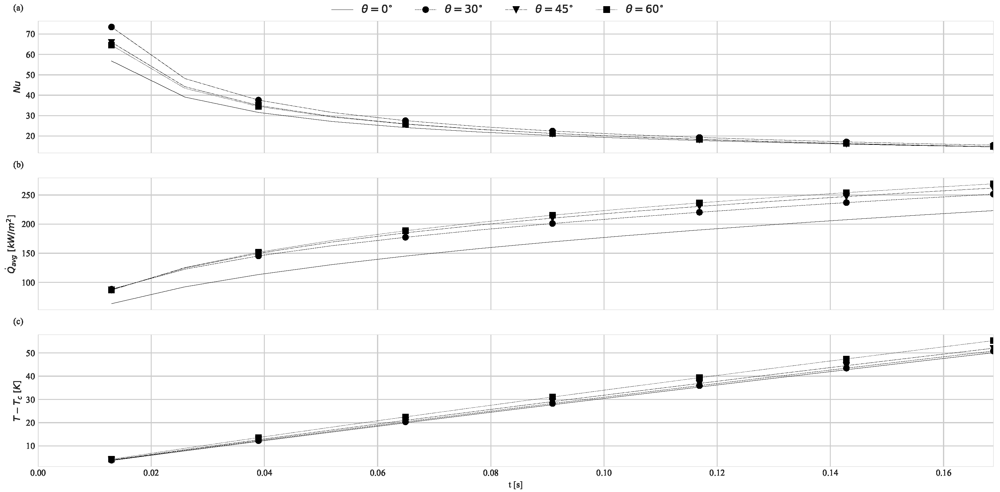
3.2.1. Geometry Impact on Natural Convection with Imposed Heat Flux

In this section, the results for the simulations where a heat flux, Q ˙ w a l l , was imposed at the base will be presented for each geometry configuration and for a flat surface. Two different heat fluxes were tested: Q ˙ w a l l = 1 × 10 5 Wm 2 and Q ˙ w a l l = 1 × 10 6 Wm 2 , resulting in Rayleigh numbers of R a = 3.8 × 10 4 and R a = 3.8 × 10 5 , respectively. Unlike the previous works [5,6,7,8,9], we specifically address the transient regime, which can be most relevant for heat exchangers operating under real cooling conditions. For example, an electronic device can be refrigerated by a tested surface in a submerged application.
For a more comprehensive understanding of the simulation results, it is interesting to analyze the temporal evolution of the variables of interest. Therefore, Figure 6 and Figure 7 present spatially averaged values for the Nusselt number ( N u ¯ L e q ), for the heat flux transferred across the base interface ( Q ˙ ¯ b a s e ), and for the temperature difference ( T a v g , b a s e T c ). It is important to note that all the averaged values presented were estimated considering the actual cavity length. As time evolves, both the heat flux and the temperature differences increase. However, in contrast, the predicted Nusselt number experiences a significant decline from the values observed at the outset. This effect can be associated with the tendency of heat transfer to approach a steady-state condition, reaching heat transfer rate values close to the imposed heat flux, while the temperature difference demonstrates an almost linear growth pattern.
From Figure 6 and Figure 7, it is evident that the structured cavities have a positive impact on the heat transfer process, leading to an increase in the Nusselt number compared to the plane surface. Among the studied geometries, Geometry 3 (with θ = 60 ° ) exhibits a more significant influence on the process. This enhanced heat transfer efficiency is further illustrated by the base temperature differences, as shown in Figure 6c and Figure 7c. Initially, the temperature differences for the geometries are lower than those observed for the plane surface, suggesting the more efficient heat transfer from the structured surfaces (resulting in higher heat fluxes). However, as the estimated heat transfer rate for the plane interface surpasses that of the structured geometries, these geometries begin to exhibit higher temperature differences than the plane surface.
The enhancement in the heat transfer process observed in Figure 6 and Figure 7 can be further investigated by analyzing both the temperature profiles and fluid motion. To perform such an analysis, we plotted both the two-dimensional temperature profiles and the streamlines for each geometry at a given instant. Figure 8 shows the plotted results for Q w a l l = 1 × 10 5 at t = 0.25 s, which is associated with a period of time in which the structured surface is shown to enhance the heat transfer process.
Starting with the temperature distributions, we observed a concentration of isothermal lines at the interface between the fluid and the solid wall, indicating higher heat transfer in those regions, particularly at the upper parts of the structured cavities (middle of the cavity). Additionally, from left to right, the isotherms appear more closely packed, indicating enhanced heat transfer. These observations confirm the performance shown in Figure 6 and Figure 7.
Now, considering the resultant fluid flow as shown in Figure 8b, we observe the fluid flow in and out of the cavities created by the geometries, thus avoiding stagnation. Upon closer observation, we note that the fluid still exhibits relatively low speed in relation to the surfaces, especially for the sharper geometry ( θ = 30 ° ). The higher velocities and the circulating fluid can be associated with the observed results in two aspects. Firstly, this observed circulation avoids the creation of stagnation zones, where the fluid would almost be stationary, effectively reducing the thermal resistance zones. Secondly, the moving fluid advects energy from the surface, thus increasing the heat transferred between the solid and the fluid.
In addition to the streamlines and temperature plots, we also estimated the vorticity at different times for the Q w a l l = 1 × 10 5 condition. The selected times shown in Figure 9 correspond to regions where the geometries exhibit better performance ( t = 0.25 s), a region where the geometries and the surfaces have similar performance ( t = 1.00 s), and, finally, regions where the plane surface surpasses the cavities ( t = 2.50 s). By comparing the results in Figure 9a with Figure 6 and Figure 8, it is evident that the higher performance of the cavities is associated with the observed vorticity, where higher levels of vorticity indicate better performance. Still considering Figure 9a, it can be seen that the smoother geometries (greater θ ) favor the formation of vortices near the surfaces, thereby aiding energy advection.
Considering the different times plotted in Figure 9, it is observable that all the configurations favor the formation of counter-rotating symmetrical vortices. Overall, the vorticity is shown to increase, indicating a higher circulation of the fluid within the domain and consequently the overall fluid rotation speed. Given the present configurations, the smoother geometries are shown to maintain the inner vortices for longer times. By comparing the results from Figure 9 with those of Figure 6, we can see that the presence of these vortices is fundamental for the better performance of the cavities. These vortices ensure that the “extra” length provided by the surface modifications remains in contact with the moving fluid, thus avoiding the creation of stagnation zones and favoring the heat transfer process.
Alternatively, the impact of structured cavities can be assessed through their effectiveness or enhancement factor, ε f , defined as the ratio between the heat transferred through the structured geometry and the plane geometry, respectively [43,44]. Figure 10 shows the evolution of the effectiveness of the geometries over time, confirming the previous results. Geometry 3 with θ = 60 ° presents the best performance, especially in the initial moments. One interesting observation concerns the evolution of effectiveness. Since the maximum heat flux is limited, it is expected that, as time advances, the effectiveness reaches a value of about 100 % due to energy conservation. In a steady-state condition, the heat flux at the solid–fluid interface should be the same as that imposed at the base. Thus, the steady-state effectiveness may not be the best parameter to evaluate the structured cavities.
Nonetheless, a transient analysis of ε f can provide interesting results. By analyzing the results displayed in Figure 10a, it is observable that the effectiveness of Geometry 3 takes longer to decay, followed by Geometry 2 and then by Geometry 1. This indicates that the heat fluxes at the solid–fluid interface of structured cavities grow faster than those for the plane interface.
Additionally, a time constant for each geometry can be estimated, providing a way to evaluate the transient performance of each geometry. Since we are measuring the time needed for ε f to reach a value of 100 % , a higher time constant means that the heat flux for the cavities reaches the value of the stationary heat flux imposed at the base faster than the plane surface. Estimated time constants are presented in Table 4 for two heat fluxes and the three cavities As expected, Geometry 3 presented a higher estimated time constant, which again serves as an indication of its better performance.
The higher effectiveness exhibited by the geometries in Figure 10, for both heat flux values, can also be observed in the evolution of the fluid temperatures, or, alternatively, of the temperature differences shown in Figure 6c and Figure 7c. Since the structured cavities demonstrate effectiveness over 100 % , it is expected that these geometries transfer heat more efficiently than the plane surface, resulting in higher temperature differences for the more “efficient” geometries. This observation further confirms the obtained results.

3.2.2. Natural Convection with Fixed Base Temperature

In addition to the previous results, we also conducted simulations of the natural convection process for five different base temperatures, T w a l l , effectively resulting in R a values ranging between 1.5 × 10 3 and 2.6 × 10 4 , considering each geometry configuration and a flat surface. The results primarily concern the average Nusselt number, N u ¯ , and the average heat flux at the solid–fluid interface, Q ˙ ¯ , throughout the transient regime.
Figure 11 illustrates the evolution of the average heat transfer rate at the solid–fluid interface. The behavior observed differs drastically betweeen each condition. For T w a l l 40 °C, all the structured cavities are shown to have a negative impact on the heat transfer process. Conversely, when considering higher wall temperatures ( T w a l l 60 °C), the enclosures begin to exhibit regions (typically at the beginning of the simulations) where an enhancement of the free-convection process through the addition of structured surfaces is noticeable. In other words, these are regions where an intensification of the heat transfer process occurs. This simulated behavior should be a direct consequence of the R a values. For small R a values, the cavities increase the solid–fluid thermal resistance due to the low flow vorticity, leading to low heat transfer rates. This behavior will be discussed further in this section.
Figure 12 and Figure 13 depict both the temperature distributions and the streamlines for T w a l l = 80 °C at t = 2.50 s (transient) and the steady-state regimes, respectively. Similar to the tests considering an imposed heat flux, the conditions of the problem favor the formation of counter-rotating symmetrical vortices. However, at the evaluated time steps, the vortices exhibit an opposite rotation compared to what was observed in the previous section, with the fluid descending at the middle section.
Despite their similarities, Figure 12 and Figure 13 show some major differences, which may help to explain the behaviors observed during the transient regime. Looking solely at the temperature distributions, a clear difference is observed in the distribution of the isothermal lines. Figure 12 presents more closely packed lines, especially near the corners of the solid–fluid interface, indicating the presence of sharper temperature gradients. Physically, this behavior translates to higher heat transfer rates. From a hydrodynamic perspective, both conditions exhibit similar behaviors, with the exception of the observed absolute fluid velocity ( | u | ), which is higher when evaluated at t = 2.50 s compared to the stationary regime. This indicates the capability to advect more energy during the transient regime.
When evaluating the impact of structured cavities on the steady-state geometry performance, we observed a negative impact compared to a plane surface, as shown in Table 5, which leads to a decrease in the Nusselt number, in accordance with previous studies such as [5,10]. These results can be associated with the stagnation of the fluid within the cavities, as can be seen in Figure 13, where the fluid reaches temperatures as close to the solid as possible, creating regions with high thermal resistance.
To better understand the negative impact of the structured cavities at a stationary state, we also plotted the local heat transfer rates at the solid–fluid interface; see Figure 14. Due to the symmetry of the problem, the results are only shown for half of the domain (from the middle section to the wall). Two distinct regions can be identified: outside and within the cavities. In the first region, the solid is in contact with fluid that exhibits relative motion to it. This motion increases the heat transferred from the solid to the fluid. In the second region, the fluid tends to stagnate, and its temperature approaches that of the solid regions. As a result, the heat transferred in this region is reduced. This behavior is observed for both regimes (transient and steady), but it is more pronounced for the steady state, resulting in a negative effect of the structured cavities. In the transient regime, the cavities produce a positive effect, enhancing the heat transfer rate from the heated surface to the fluid.

4. Conclusions

In this paper, we introduced modifications to an existing thermal LBM model for simulating conjugate heat transfer processes [24], aimed at accounting for the local and temporal variations in the thermophysical properties. By working with the conservative form of the energy conservation equation written on the basis of the temperature and constant-pressure specific heat, we derived a source term that encompasses both the time and spatial variations in the domain properties. We also proposed the calculation of the reference temperature for each time step. These modifications are the main novelty of the paper and enabled the numerical simulation of the natural convection process in an enclosure with structured cavities as a function of time. The following are the main conclusions of the paper.
1. The proposed LBM model was validated through the solution of three benchmark problems, including purely diffusion, advection–diffusion, and free-convection problems. Overall, the proposed modified model presented consistently low relative errors compared to the reference analytical and numerical solutions.
2. Furthermore, the proposed LBM model was employed to investigate the natural convection phenomenon within an enclosure with structured cavities. Two principal simulations were undertaken: first, cases involving the imposition of a uniform heat flux at the domain base (solid medium); second, in a more traditional way, the imposition of a uniform base temperature was also studied.
3. Alternatively to previous works, we focused our analysis on the transient regime, which revealed interesting results. In both simulations, an enhancement of the free-convection process was perceived for the structured surfaces, mainly for higher R a . As discussed before, these results are associated with higher vorticities, which favors the fluid circulation within the domain, thus preventing its stagnation inside the cavities. This kind of result is very scarce in the open literature.
4. Additionally, we also examined the stationary regimes (only for the second simulation case). In these circumstances, the base problem (an enclosure with a plane interface) was shown to generate higher heat transfer rates, and consequently higher Nusselt numbers, when compared to the structured surfaces, supporting the findings from prior research [5,10]. Contrary to the transient cases, in these circumstances, some portion of the fluid stagnates inside the cavities, essentially creating additional thermal resistances, ultimately reducing the heat transfer rates.
In summary, the natural convection simulation within an enclosure with a structured surface provided interesting insights regarding this heat transfer process. First, in accordance with the previous works [5,10], the presence of a structured surface was shown to have a negative impact on the stationary heat transfer process, favoring the stagnation of the fluid between the cavities. On the other hand, when considering transient regimes, where most of the practical application occurs, the structured surfaces were shown to present a positive impact, in particular for what concerns higher R a , since in this condition no fluid stagnation within the cavities was perceived.

Author Contributions

Conceptualization, V.A.M., I.T.M., and L.C.-G.; Methodology, V.A.M., I.T.M., D.C.M., L.C.-G. and E.P.B.F.; Software, V.A.M. and I.T.M.; Validation, V.A.M. and I.T.M.; Formal Analysis, V.A.M., I.T.M., D.C.M., L.C.-G. and E.P.B.F.; Resources, E.P.B.F.; Writing—Original Draft Preparation, V.A.M. and I.T.M.; Writing—Review and Editing, V.A.M., I.T.M., D.C.M., L.C.-G. and E.P.B.F.; Supervision, L.C.-G.; Project Administration, D.C.M., L.C.-G. and E.P.B.F. All authors have read and agreed to the published version of the manuscript.

Funding

This research received no external funding.

Data Availability Statement

Data are available under request.

Acknowledgments

The authors acknowledge the support received from the CAPES (Coordenação de Aperfeiçoamento de Pessoal de Nível Superior, Brasil; Finance Code 001; process 88887.805775/2023-00), FAPESP grants (2022/12257-5, 2022/15765-1, and 2023/02383-6), and FAPEMIG and CNPq grants (305771/2023-0).

Conflicts of Interest

The authors declare no conflict of interest.

Appendix A. Chapman–Enskog Analysis

The Chapman–Enskog analysis for the proposed LBE with the source term is performed in this section. First, we start by considering that the source term S g i = 1 Δ t 2 τ T w i S g ; consequently, h 0 = ( i g i + 0.5 δ t S g ) .
For the sake of clarity, the index notation will be used here, α , β , and γ being the Cartesian coordinates, as well as the short notation of derivatives ( t , α , α β , etc.). Starting from the thermal lattice Boltzmann equation for discrete velocity directions, considering the BGK collision operator and the source term,
g i ( x α + c i α δ t , t + δ t ) g i ( x α , t ) = δ t τ T g i ( x α , t ) g i e q ( x α , t ) + δ t S g i .
Expanding g i ( x α + c i α δ t , t + δ t ) in Taylor series considering only the second-order terms, the LBE becomes
δ t t g i + c i α α g i + δ t 2 2 t t g i + 2 c i α t α g i + c i α 2 α α g i + O ( δ t ) 3 = δ t τ T g i g i e q + δ t S g i ,
Next, the temporal and spatial derivatives and the distribution functions are expanded in terms of the Knudsen number K n . Defining ϵ to indicate the Knudsen order terms (for example, ϵ n K n n ) and expanding g i as a perturbation series around g i e q :
ϵ t ( 1 ) + ϵ 2 t ( 2 ) + c i α ϵ α ( 1 ) g i ( 0 ) + ϵ g ( 1 ) + ϵ 2 g i ( 2 ) + . . . δ t 2 ϵ t ( 1 ) + ϵ 2 t ( 2 ) 2 + 2 c i α ϵ α ( 1 ) ϵ t ( 1 ) + ϵ 2 t ( 2 ) + c i α 2 ϵ α ( 1 ) 2 g i ( 0 ) + ϵ g ( 1 ) + ϵ 2 g i ( 2 ) + . . . O ( δ t ) 3 = 1 τ T g i ( 0 ) + ϵ g ( 1 ) + ϵ 2 g i ( 2 ) g i e q + ϵ ( 1 ) S g i ( 1 )
Neglecting terms with order greater than ϵ 3 , the final expression becomes
ϵ 0 1 τ T g i ( 0 ) g i e q + ϵ 1 t ( 1 ) g i ( 0 ) + c i α α ( 1 ) g i ( 0 ) + g i ( 1 ) τ T S g i ( 1 ) + . . . ϵ 2 t ( 1 ) g i ( 1 ) + t ( 2 ) g i ( 0 ) + c i α α ( 1 ) g i ( 1 ) + δ t 2 t 2 ( 1 ) g i ( 0 ) + 2 c i α t α ( 1 ) g i ( 0 ) + c i α 2 α 2 ( 1 ) g i ( 0 ) + g i ( 2 ) τ T = 0
Splitting in relation to the order of ϵ and re-ordering the expressions, we have
ϵ 0 : g i ( 0 ) = g i e q
ϵ 1 : t ( 1 ) + c i α α ( 1 ) g i ( 0 ) = g i ( 1 ) τ T + S g i ( 1 )
ϵ 2 : t ( 2 ) g i ( 0 ) + t ( 1 ) + c i α α ( 1 ) g i ( 1 ) + Δ t 2 t ( 1 ) + c i α α ( 1 ) 2 g i ( 0 ) = g i ( 2 ) τ T
Taking the zeroth and first moments of Equation (A6) and substituting the source term,
0 t h : t ( 1 ) h 0 + α ( 1 ) u α h 0 = S g ( 1 ) 1 s t : t ( 1 ) u α h 0 + c s 2 α ( 1 ) h 0 = 1 τ T g i ( 1 ) c i α
Substituting Equation (A6) in Equation (A7), taking the zeroth moment of the resultant equation, and re-ordering,
α ( 2 ) h 0 + α ( 1 ) Δ t 2 τ T c s 2 α ( 1 ) h 0 + α ( 1 ) Δ t 2 τ T t ( 1 ) u α h 0 = 1 4 1 Δ t 2 τ T Δ t t ( 1 ) S g ( 1 )
Summing Equation (A9) with the 0th moment in Equation (A8) in the respective ϵ order,
ϵ t ( 1 ) + ϵ 2 t ( 2 ) h 0 + ϵ α ( 1 ) h 0 u α + ϵ α ( 1 ) Δ t 2 τ T c s 2 ϵ α ( 1 ) h 0 + E = . . . ϵ 2 1 4 1 Δ t 2 τ T Δ t t ( 1 ) S g ( 1 ) + ϵ S g ( 1 )
where E = α ( 1 ) Δ t 2 τ T t ( 1 ) u α h 0 is the error term in the analysis. Recuperating the derivatives and macroscopic quantities from the expansion in ϵ ,
t h 0 + · ( u h 0 ) = ( α h 0 ) + S g = ( α h 0 ) k ρ c P 0 h 0 1 σ
Thus, we can see that the proposed method indeed recovers Equation (16).

Appendix B. Analytical Solution Heat Diffusion between Three Solids

The analytical solution for this problem is provided in the form of Equation (A12), where Θ = ( T T w 2 ) / ( T w 1 T w 2 ) , ξ 1 = x / x 1 , ξ 2 = ( x d 1 ) / x 2 , ξ 3 = [ x ( d 1 + d 2 ) ] / x 3 , τ = t / t 0 , δ 1 = α C u t 0 / ( d 1 2 ) , δ 2 = α S i t 0 / ( d 2 2 ) , δ 3 = α A l t 0 / ( d 3 2 ) , κ 1 = K C u / d 1 , κ 2 = K S i / d 1 , and κ 3 = K A l / d 1 , with t 0 being a reference time set as the total studied time and d i the length of each layer.
Θ ( ξ i , τ ) = Φ ( ξ i ) ϕ ( ξ i , τ )
The term Φ ( ζ i ) refers to the steady-state solution for the problem and is provided by Equation (A13).
Φ ( ξ 1 ) = 1 ( Δ Θ ) 1 ξ 1 , if   0 < ξ 1 1 ; Φ ( ξ 2 ) = 1 ( Δ Θ ) 1 ( Δ Θ ) 2 ξ 2 , if   0 < ξ 2 1 ; Φ ( ξ 3 ) = 1 ( Δ Θ ) 1 ( Δ Θ ) 2 ( Δ Θ ) 3 ξ 3 , if   0 < ξ 3 1 ;
where
( Δ Θ ) i = ( 1 / κ i ) / ( 1 / κ 1 + 1 / κ 2 + 1 / κ 3 )
The term ϕ ( ξ i , τ ) is the unsteady solution for the problem that satisfies the boundary conditions and is provided by Equation (A14).
ϕ ( ξ 1 , τ ) = n = 0 A n e λ n 2 δ 1 τ sin ( λ n ξ 1 ) , if   0 < ξ 1 1 ; ϕ ( ξ 2 , τ ) = Δ 1 n = 0 A n e λ n 2 δ 2 τ α n sin δ 1 δ 2 λ n ξ 2 + β n cos δ 1 δ 2 λ n ξ 2 , if   0 < ξ 2 1 ; ϕ ( ξ 3 , τ ) = Δ 2 n = 0 A n e λ n 2 δ 3 τ α ¯ n sin δ 1 δ 3 λ n ξ 3 + β ¯ n cos δ 1 δ 3 λ n ξ 3 , if   0 < ξ 3 1 ;
where
Δ i = κ 1 κ i + 1 δ i + 1 δ 1 ; α n = cos ( λ n ) ; β n = sin ( λ n ) / Δ 1 ; α ¯ n = cos ( λ n ) cos δ 1 δ 2 λ n sin ( λ n ) sin δ 1 δ 2 λ n / Δ 1 ; β ¯ n = cos ( λ n ) sin δ 1 δ 2 λ n Δ 1 Δ 2 sin ( λ n ) cos δ 1 δ 2 λ n / Δ 2 ; M n = κ 1 κ 2 2 + κ 1 κ 3 cos 2 ( λ n ) + sin 2 ( λ n ) / Δ 1 2 2 + κ 1 κ 2 ( α ¯ n 2 + β ¯ n 2 ) 2 A n = κ 2 κ 3 λ n M n
Finally, λ n indicates the eigenvalues that satisfy the relation shown in Equation (A15)
tan ( λ n ) = Δ 1 tan δ 1 δ 2 λ n + Δ 2 tan δ 1 δ 3 λ n 1 Δ 2 Δ 1 tan δ 1 δ 2 λ n tan δ 1 δ 3 λ n

Appendix C. Analytical Solution Convection–Diffusion with a Flat Interface

The solution for this problem is provided by Equation (A16), 1 being the lower fluid (water in the case treated) and 2 the upper one (ethanol).
T ( x , y , t ) = T 0 + Δ T · R e e j ( K x + ω t ) γ 1 e λ 1 y + 1 γ 1 e λ 1 y , if   0 y h ; T ( x , y , t ) = T 0 + Δ T · R e e j ( K x + ω t ) γ 2 e λ 2 y + 1 γ 2 e λ 2 H e λ 2 ( H y ) , if   h < y H ;
With R e referring to the real part of the solution, and with the following coefficients:
σ = ( ρ c p ) 2 ( ρ c p ) 1 ; κ = α 2 α 1 ; λ 1 = K 1 + j ω + U 0 K K 2 α 1 ; λ 2 = K 1 + j ω + U 0 K K 2 α 2 a 1 = e λ 1 h ; a 2 = e λ 2 h ; a 3 = e λ 2 H γ 1 = λ 1 ( a 3 2 a 2 2 ) + κ σ λ 2 ( 2 a 1 a 2 a 3 a 2 2 a 3 2 ) ( λ 1 + κ σ λ 2 ) ( a 1 2 a 3 2 a 2 2 ) ( λ 1 κ σ λ 2 ) ( a 1 2 a 2 2 a 3 2 ) γ 2 = λ 1 ( a 1 2 a 3 + a 3 2 a 1 a 2 ) + κ σ λ 2 ( a 1 2 1 ) a 3 ( λ 1 + κ σ λ 2 ) ( a 1 2 a 3 2 a 2 2 ) ( λ 1 κ σ λ 2 ) ( a 1 2 a 2 2 a 3 2 )

Appendix D. Nusselt Number Calculation

Two primary approaches for evaluating the Nusselt number can be employed. The first method estimates N u based on the projected length of the geometries, resulting in N u ¯ L . The second approach calculates N u using the actual length of the cavity, leading to N u ¯ L e q . Both methods yield similar outcomes in identifying the “better” surface. However, calculations based on the projected area consistently produce much lower values compared to those observed for the plane interface. Conversely, when considering the real interface length, the N u values are found to be closer to those of the plane interface. Nonetheless, the average Nusselt number can be estimated by integrating the non-dimensional temperature, Equation (A17), along the solid–fluid interface, resulting in Equation (A18), with both approaches differing with regard to the integration domain.
Θ ( x ) = T s ( x ) T c o l d Δ T ; Δ T = Q w a l l L k f
N u ¯ = 0 L 1 Θ ( x ) d x

References

  1. Bejan, A.; Kraus, A. Heat Transfer Handbook; Wiley: Hoboken, NJ, USA, 2003; Volume 1. [Google Scholar]
  2. Aneesh, A.; Sharma, A.; Srivastava, A.; Vyas, K.; Chaudhuri, P. Thermal-hydraulic characteristics and performance of 3D straight channel based printed circuit heat exchanger. Appl. Therm. Eng. 2016, 98, 474–482. [Google Scholar] [CrossRef]
  3. Buchberg, H.; Catton, I.; Edwards, D.K. Natural Convection in Enclosed Spaces—A Review of Application to Solar Energy Collection. J. Heat Transf. 1976, 98, 182–188. [Google Scholar] [CrossRef]
  4. Baïri, A.; Zarco-Pernia, E.; De María, J.M.G. A review on natural convection in enclosures for engineering applications. The particular case of the parallelogrammic diode cavity. Appl. Therm. Eng. 2014, 63, 304–322. [Google Scholar] [CrossRef]
  5. Pretot, S.; Zeghmati, B.; Caminat, P. Influence of surface roughness on natural convection above a horizontal plate. Adv. Eng. Softw. 2000, 31, 793–801. [Google Scholar] [CrossRef]
  6. Oosthuizen, P.H. A numerical study of laminar and turbulent natural convective heat transfer from an isothermal vertical plate with a wavy surface. In Proceedings of the ASME International Mechanical Engineering Congress and Exposition, Vancouver, BC, Canada, 12–18 November 2010; Volume 44441, pp. 1481–1486. [Google Scholar]
  7. Oosthuizen, P. Natural convective heat transfer from an inclined isothermal plate with a wavy surface. In Proceedings of the 42nd AIAA Thermophysics Conference, Honolulu, HI, USA, 27–30 June 2011; p. 3943. [Google Scholar]
  8. Oosthuizen, P.H.; Kalendar, A. A numerical study of the effect of spaced triangular surface waves on natural convective heat transfer from an upward facing heated horizontal isothermal surface. In Proceedings of the 5th Thermal and Fluids Engineering Conference (TFEC), New Orleans, LA, USA, 5–8 April 2020. [Google Scholar]
  9. Hussain, S.; Kalendar, A.; Rafique, M.Z.; Oosthuizen, P.H. Assessment of thermal characteristics of square wavy plates. Heat Transf. 2020, 49, 3742–3757. [Google Scholar] [CrossRef]
  10. Hossain, M.; Rees, D.A.S. Combined heat and mass transfer in natural convection flow from a vertical wavy surface. Acta Mech. 1999, 136, 133–141. [Google Scholar] [CrossRef]
  11. Siddiqa, S.; Hossain, M.; Saha, S.C. The effect of thermal radiation on the natural convection boundary layer flow over a wavy horizontal surface. Int. J. Therm. Sci. 2014, 84, 143–150. [Google Scholar] [CrossRef]
  12. Siddiqa, S.; Hossain, M.A.; Gorla, R.S.R. Natural convection flow of viscous fluid over triangular wavy horizontal surface. Comput. Fluids 2015, 106, 130–134. [Google Scholar] [CrossRef]
  13. Oosthuizen, P.H.; Paul, J.T. A numerical study of natural convective heat transfer from an inclined isothermal plate having a square wave surface. In Proceedings of the ASME International Mechanical Engineering Congress and Exposition, Denver, CO, USA, 11–17 November 2011; Volume 54969, pp. 445–450. [Google Scholar]
  14. Perelman, T. On conjugated problems of heat transfer. Int. J. Heat Mass Transf. 1961, 3, 293–303. [Google Scholar] [CrossRef]
  15. Armero, F.; Simo, J. A new unconditionally stable fractional step method for non-linear coupled thermomechanical problems. Int. J. Numer. Methods Eng. 1992, 35, 737–766. [Google Scholar] [CrossRef]
  16. Giles, M.B. Stability analysis of numerical interface conditions in fluid–structure thermal analysis. Int. J. Numer. Methods Fluids 1997, 25, 421–436. [Google Scholar] [CrossRef]
  17. Roe, B.; Jaiman, R.; Haselbacher, A.; Geubelle, P. Combined interface boundary condition method for coupled thermal simulations. Int. J. Numer. Methods Fluids 2008, 57, 329–354. [Google Scholar] [CrossRef]
  18. Zhang, J.; Yang, C.; Mao, Z.S. Unsteady conjugate mass transfer from a spherical drop in simple extensional creeping flow. Chem. Eng. Sci. 2012, 79, 29–40. [Google Scholar] [CrossRef]
  19. Succi, S. The Lattice Boltzmann Equation: For Fluid Dynamics and Beyond; Oxford University Press: Oxford, UK, 2001. [Google Scholar]
  20. Korba, D.; Wang, N.; Li, L. Accuracy of interface schemes for conjugate heat and mass transfer in the lattice Boltzmann method. Int. J. Heat Mass Transf. 2020, 156, 119694. [Google Scholar] [CrossRef]
  21. Li, L.; Chen, C.; Mei, R.; Klausner, J.F. Conjugate heat and mass transfer in the lattice Boltzmann equation method. Phys. Rev. E 2014, 89, 043308. [Google Scholar] [CrossRef]
  22. Karani, H.; Huber, C. Lattice Boltzmann formulation for conjugate heat transfer in heterogeneous media. Phys. Rev. E 2015, 91, 023304. [Google Scholar] [CrossRef] [PubMed]
  23. Rihab, H.; Moudhaffar, N.; Sassi, B.N.; Patrick, P. Enthalpic lattice Boltzmann formulation for unsteady heat conduction in heterogeneous media. Int. J. Heat Mass Transf. 2016, 100, 728–736. [Google Scholar] [CrossRef]
  24. Chen, S.; Yan, Y.; Gong, W. A simple lattice Boltzmann model for conjugate heat transfer research. Int. J. Heat Mass Transf. 2017, 107, 862–870. [Google Scholar] [CrossRef]
  25. Hosseini, S.; Darabiha, N.; Thévenin, D. Lattice Boltzmann advection-diffusion model for conjugate heat transfer in heterogeneous media. Int. J. Heat Mass Transf. 2019, 132, 906–919. [Google Scholar] [CrossRef]
  26. Yang, L.; Shu, C.; Yang, W.; Wu, J. Simulation of conjugate heat transfer problems by lattice Boltzmann flux solver. Int. J. Heat Mass Transf. 2019, 137, 895–907. [Google Scholar] [CrossRef]
  27. Kiani-Oshtorjani, M.; Kiani-Oshtorjani, M.; Mikkola, A.; Jalali, P. Conjugate heat transfer in isolated granular clusters with interstitial fluid using lattice Boltzmann method. Int. J. Heat Mass Transf. 2022, 187, 122539. [Google Scholar] [CrossRef]
  28. Bird, R.B.; Stewart, W.E.; Lightfoot, E.N. Transport Phenomena, 2nd ed.; John Wiley & Sons, Inc.: Hoboken, NJ, USA, 2002. [Google Scholar]
  29. Martins, I.T.; Alvariño, P.F.; Cabezas-Gómez, L. Lattice Boltzmann method for simulating transport phenomena avoiding the use of lattice units. J. Braz. Soc. Mech. Sci. Eng. 2024, 46, 333. [Google Scholar] [CrossRef]
  30. Bhatnagar, P.L.; Gross, E.P.; Krook, M. A Model for Collision Processes in Gases. I. Small Amplitude Processes in Charged and Neutral One-Component Systems. Phys. Rev. 1954, 94, 511–525. [Google Scholar] [CrossRef]
  31. Krüger, T.; Kusumaatmaja, H.; Kuzmin, A.; Shardt, O.; Silva, G.; Viggen, E. The Lattice Boltzmann Method: Principles and Practice; Springer International Publishing: Berlin/Heidelberg, Germany, 2017. [Google Scholar]
  32. Qian, Y.H.; D’Humieres, D.; Lalleman, P. Lattice BGK Models for Navier-Stokes Equation. Europhys. Lett. 1992, 17, 479–484. [Google Scholar] [CrossRef]
  33. Guo, Z.; Shu, C. Lattice Boltzmann Method and Its Applications in Engineering; World Scientific Publishing Co. Pte. Ltd.: Singapore, 2013. [Google Scholar]
  34. Guo, Z.; Zheng, C.; Shi, B. Discrete lattice effects on the forcing term in the lattice Boltzmann method. Phys. Rev. E 2002, 65, 046308. [Google Scholar] [CrossRef] [PubMed]
  35. Chapman, S.; Cowling, T.G. The Mathematical Theory of Non-Uniform Gases, 2nd ed.; Cambridge University Press: Cambridge, UK, 1952. [Google Scholar]
  36. Klein, S.A. EES – Engineering Equation Solver, Version 11.444 (2022-09-29); Computer Software; F-Chart Software: Madison, WI, USA, 2022. [Google Scholar]
  37. Seta, T. Implicit temperature correction-based immersed boundary-thermal lattice Boltzmannmethod for the simulation of natural convection. Phys. Rev. E 2013, 87, 063304. [Google Scholar] [CrossRef]
  38. Chai, Z.; Zhao, T.S. Nonequilibrium scheme for computing the flux of the convection-diffusion equation in theframework of the lattice Boltzmann method. Phys. Rev. E 2014, 90, 013305. [Google Scholar] [CrossRef] [PubMed]
  39. Martins, I.T.; Matsuda, V.A.; Cabezas-Gómez, L. A new Neumann boundary condition scheme for the thermal lattice Boltzmann method. J. Int. Commun. Heat Mass Transf. 2023, preprint. [Google Scholar]
  40. Sun, Y.; Wichman, I.S. On transient heat conduction in a one-dimensional composite slab. Int. J. Heat Mass Transf. 2004, 47, 1555–1559. [Google Scholar] [CrossRef]
  41. Cheikh, N.B.; Beya, B.B.; Lili, T. Influence of thermal boundary conditions on natural convection in a square enclosure partially heated from below. Int. Commun. Heat Mass Transf. 2007, 34, 369–379. [Google Scholar] [CrossRef]
  42. Moreira, D.C.; Nascimento, V.; Ribatski, G.; Kandlikar, S. Combining liquid inertia and evaporation momentum forces to achieve flow boiling inversion and performance enhancement in asymmetric Dual V-groove microchannels. Int. J. Heat Mass Transf. 2022, 194, 123009. [Google Scholar] [CrossRef]
  43. Kakac, S.; Bergles, A.; Mayinger, F.; Yuncu, H. Heat transfer enhancement of heat exchangers. Dry. Technol. 2000, 18, 837–838. [Google Scholar]
  44. Lienhard, J.H., IV; Lienhard, J.H., V. A Heat Transfer Textbook, 5th ed.; Phlogiston Press: Cambridge, MA, USA, 2020; Version 5.10. [Google Scholar]
Figure 1. Transient solid heat diffusion: temperature distribution along the x-direction for various times.
Inventions 09 00057 g001
Figure 2. Transient results for heat convection–diffusion at t = 0.75 Γ : (a) temperature distribution; (b) temperature profiles along different x-axis cuts.
Inventions 09 00057 g002
Figure 3. Natural convection benchmark problem considering conjugate heat transfer.
Inventions 09 00057 g003
Figure 4. Results for the natural convection benchmark test ( Δ x = 6.25 · 10 6 ): (a) temperature distribution; (b) streamlines.
Inventions 09 00057 g004
Figure 5. Geometry scheme and dimensions.
Inventions 09 00057 g005
Figure 6. Q ˙ w a l l = 1 · 10 5 [ W / m 2 ] : (a) N u L e q ¯ ; (b) Q ˙ ¯ b a s e ; (c) T a v g , b a s e T c .
Inventions 09 00057 g006
Figure 7. Q ˙ w a l l = 1 · 10 6 [ W / m 2 ] : (a) N u L e q ¯ ; (b) Q ˙ ¯ b a s e ; (c) T a v g , b a s e T c .
Inventions 09 00057 g007
Figure 8. Results for Q w a l l = 1 · 10 5 at t = 0.25 s: (a) temperature distribution; (b) streamlines. The number index refers to the geometry angles. The caption numbers are a reference to the geometries.
Inventions 09 00057 g008
Figure 9. Vorticity for Q w a l l = 1 · 10 5 : (a) t = 0.25 s; (b) t = 1.00 s; (c) t = 2.50 s. The caption numbers are a reference to the geometries.
Inventions 09 00057 g009
Figure 10. Surface effectiveness evolution: (a) Q ˙ w a l l = 1 · 10 5 [ W / m 2 ] ; (b) Q ˙ w a l l = 1 · 10 6 [ W / m 2 ] .
Inventions 09 00057 g010
Figure 11. Average heat transfer rate time evolution: (a) T w a l l = 30 °C; (b) T w a l l = 40 °C; (c) T w a l l = 60 °C; (d) T w a l l = 80 °C; (e) T w a l l = 90 °C.
Inventions 09 00057 g011
Figure 12. Simulation results for T w a l l = 80 °C at t = 2.50 s (transient regime): (a) temperature field distribution; (b) streamlines. The caption numbers are a reference to the geometries.
Inventions 09 00057 g012
Figure 13. Simulation results for T w a l l = 80 °C and the stationary regime: (a) temperature field distribution; (b) streamlines. The caption numbers are a reference to the geometries.
Inventions 09 00057 g013
Figure 14. Heat transfer rate at the fluid–solid interface: (a) T w a l l = 30 °C; (b) T w a l l = 40 °C; (c) T w a l l = 60 °C; (d) T w a l l = 80 °C; (e) T w a l l = 90 °C.
Inventions 09 00057 g014
Table 1. Total errors for the convection–diffusion problem at different times.
t [ s ] Global Errors · 10 2 [ % ] t [ s ] Global Errors · 10 2 [ % ]
100.0 0.0152 900.0 0.0435
200.0 0.0337 1000.0 0.0424
300.0 0.0434 1100.0 0.0414
400.0 0.0472 1200.0 0.0407
500.0 0.0481 1300.0 0.0401
600.0 0.0474 1400.0 0.0396
700.0 0.0462 1500.0 0.0393
800.0 0.0448 1600.0 0.0391
Table 2. Global errors for the convection–diffusion problem at different times.
t / Γ Global Errors · 10 2 [ % ] t / Γ Global Errors · 10 2 [ % ]
0.125 2.1 0.625 1.65
0.250 1.58 0.750 1.65
0.375 1.65 0.875 1.65
0.500 1.66 1.000 1.65
Table 3. Nusselt number errors for a natural convection problem.
Reference Nusselt Number: Nu = 3.80
Δ x · 10 5 [m] Nu ¯ Errors  Nu ¯  [%]
2.500 3.72 2.17
1.250 3.75 1.39
0.625 3.80 0.07
Table 4. Time constant estimation.
Q wall [ W / m 2 ] 1 · 10 5 1 · 10 6
θ °304560304560
t a u [ s ] 0.22 0.34 0.48 0.06 0.10 0.18
Table 5. Geometry comparison.
T wall = 30 ° C Ra L = 1.5 · 10 3 T wall = 40 ° C Ra L = 4.1 · 10 3 T wall = 60 ° C Ra L = 1.2 · 10 4 T wall = 80 ° C Ra L = 2.4 · 10 4 T wall = 90 ° C Ra L = 2.6 · 10 4
θ °03045600304560030456003045600304560
N u ¯ L e q 1.030.940.840.81.030.940.840.81.861.741.551.432.752.562.282.13.042.842.522.32
Q ¯ [ kWm 2 ] 3.143.012.892.636.366.15.865.3323.2923.021.9719.4152.4651.8649.443.7568.2567.4664.2556.83
Disclaimer/Publisher’s Note: The statements, opinions and data contained in all publications are solely those of the individual author(s) and contributor(s) and not of MDPI and/or the editor(s). MDPI and/or the editor(s) disclaim responsibility for any injury to people or property resulting from any ideas, methods, instructions or products referred to in the content.

