

An Assessment of the Role of the Timex Sampling Strategy on the Precision of Shoreline Detection Analysis

1
Deakin Marine Research and Innovation Centre, School of Life and Environmental Sciences, Deakin University, Burwood, VIC 3125, Australia
2
Ryan Institute for Environmental, Marine and Energy Research, University of Galway, H91 TK33 Galway, Ireland
3
Discipline of Geography, University of Galway, H91 TK33 Galway, Ireland
4
College of Science & Engineering, University of Galway, H91 TK33 Galway, Ireland
5
MaREI Research Centre for Energy, Climate and Marine, National University of Ireland Galway, T23 XE1 Cork, Ireland
*
Author to whom correspondence should be addressed.
Coasts 2024, 4(2), 347-365; https://doi.org/10.3390/coasts4020018
Submission received: 9 February 2024
/
Revised: 12 March 2024
/
Accepted: 22 April 2024
/
Published: 9 May 2024
Abstract
:Remote video imagery using shoreline edge detection is widely used in coastal monitoring in order to acquire measurements of nearshore and swash features. Some of these systems are constrained by their long setup time, positioning requirements and considerable hardware costs. As such, there is a need for an autonomous low-cost system (~EUR 500), such as Timex cameras, that can be rapidly deployed in the field, while still producing the outcomes required for coastal monitoring. This research presents an assessment of the effect of the sampling strategy (time-lapse intervals) on the precision of shoreline detection for two low-cost cameras located in a remote coastal area in western Ireland, overlooking a dissipative beach–dune system. The analysis shows that RMSD in the detected shoreline is similar to other studies for sampling intervals ranging between 1 s and 30 s (i.e., RMSDmean for Camera 1 = 1.4 m and Camera 2 = 0.9 m), and an increase in the sampling interval from 1 s to 30 s had no significant adverse effect on the precision of shoreline detection. The research shows that depending on the intended use of the detected shorelines, the current standard of 1 s image sampling interval when using Timex cameras can be increased up to 30 s without any significant loss of accuracy. This positively impacts battery life and memory storage, making the systems more autonomous; for example, the battery life increased from ~10 days to ~100 days when the sampling interval was increased from 1 to 5 s.
1. Introduction
Coastal zones are unique and dynamic environments of high economic and ecological importance, with approximately 31% of all coastal zones containing sandy beaches [1]. These are particularly dynamic and some of the most responsive environments on Earth. In order to gain a better understanding of their dynamics, repeat topographic surveys have become an essential part of coastal zone research, coastal engineering applications, and coastal zone management. Indeed, survey data and their analysis are valuable resources for quantifying long-term trends such as the erosion and/or accretion of beaches [2,3,4], beach and dune response–recovery patterns due to storm events [5,6,7], and impacts of engineering works [8,9], as well as identifying dynamic features such as beach cusps and nearshore bars [10,11,12]. The site-specific nature and variability in coastal response means that coastal monitoring programmes should, preferably, span years to decades and include local environmental factors (e.g., coastal morphology, sediment budget, rates of sea-level rise, nearshore and swash dynamics) [13]. For many decades, the logistics (e.g., time, cost, travel) of field monitoring precluded our ability to collect high-temporal-resolution datasets, but the advent of commercial, low-cost camera systems in coastal science has removed this obstacle.
In order to better understand and characterise the different coastal processes occurring in the nearshore and swash zones, longer datasets with higher spatial and temporal resolution are preferable. These can be obtained using indirect measurement/remote sensing techniques which were originally developed to facilitate the collection of data in the nearshore [14]. Remote sensing techniques provide an attractive alternative to direct measuring techniques, especially in difficult environments, extreme conditions, or to achieve high temporal resolutions. A range of indirect measuring techniques is already used in coastal areas, including active sensors, e.g., LiDAR [15,16] and RADAR, and passive sensors, e.g., time-lapse [10], video [17,18] and infrared cameras [19]; smartphones [20,21]; and unmanned aerial vehicles (UAVs) [22,23,24]. The conventional products that can be extracted from passive sensors are (1) snapshot: an instantaneous image; (2) Timex: a single image averaging multiple snapshot images over one period, typically 10 or 15 min; (3) Variance: similarly to Timex images, variance images contain the standard deviation computed in time from the same set of snapshots used to generate the Timex image; and (4) Timestack: intensity values saved at each time step at a selected array of pixels (i.e., transect) from a snapshot. These approaches have been used to monitor a broad range of coastal and nearshore features including, but not limited to, the extraction of beach and nearshore bathymetry [25,26], nearshore hydrodynamics [27,28], the formation and displacement of sand bars [29,30,31], and beach face morphodynamics [32,33,34,35].
In addition, passive sensors such as time-lapse cameras and video cameras have been used to detect and delineate shoreline positions [36,37,38]. Identifying shoreline positions and their shift in response to hydrodynamics is essential to coastal scientists, engineers, and managers [39]. Data of where the current shoreline position is, where it has been in the past, and being able to predict where it will be in the future can inform coastal protection strategies [40]. It also provides the ability to calibrate and verify numerical models [41], assess sea-level change [42], and identify high-risk coastal zones [43]. Indeed, the detection of shorelines from processed video images has become a standard tool in nearshore studies [44], especially since the growth of the ARGUS system [45].
For most remotely sensed systems, the sensor is in a fixed location and collects oblique images of the nearshore. The fixed location of the sensor means that only the lens characteristics and ground control points (GCPs) are required to create a georectified image [46]. From this, objective information can be subtracted from the oblique images (e.g., shoreline positions). The shoreline itself can be defined in optical images as the time-varying interface between ‘wet’ pixels, representing the ocean surface, and ‘dry’ pixels, indicating beach sediments [47]. In order to identify shoreline positions from optical images, several approaches have been proposed: localised maxima in the image intensity (SLIM) [48]; pixel clustering based on HUE and intensity (PIC) [25]; divergence in RGB colour channels [21,49]; and machine learning techniques [50]. Each of these techniques manipulates the optical information in a slightly different manner to objectively define a proxy shoreline feature.
Finding a compromise between the optimum sampling rate and the time period over which to average the images remains an ongoing challenge in this research area; Refs. [47,51] found that the sampling interval of 1 Hz over 10 min has become a standard procedure but there has been no investigation into the performance of Timex images with different sampling rates. To the best of our knowledge, no analysis has been carried out to investigate the optimum interval of Timex images in coastal research applications. Such an investigation can benefit low-cost monitoring systems, as a potential increase in sampling intervals can dramatically improve current limitations on battery requirements and storage capacity.
This study addresses this gap by examining the role of sampling strategy on the accuracy of shoreline detection analysis. Specifically, we assess the errors in shoreline detection resulting from different sampling intervals, i.e., 1 s, 3 s, 5 s, 10 s, 20 s, and 30 s, using Timex images. The justification for this research is the drive to create a more autonomous system with a larger sampling interval resulting in longer battery life and lower storage requirements, meaning less user intervention. Timex images were created from high-resolution oblique imagery and shoreline positions were determined from the different Timex images. Hence, the focus lies in evaluating how sampling strategies impact shoreline detection accuracy, aiming to provide guidance for selecting optimal temporal resolutions for processing Timex images.
Timex images are captured by a low-cost (circa EUR 500) monitoring system (e.g., an off-the-shelf time-lapse camera) and can be rapidly deployed in the field and/or in remote areas, which can reduce the initial capital and investment in monitoring systems and can lead to a fully autonomous system (e.g., no external power source or hardware). The internal batteries from off-the-shelf time-lapse cameras are often small, and data are stored on SD cards with storage in the order of hundreds of GB. This makes them fully autonomous but also reduces the time period that they can sample at field sites.
2. Materials and Methods
2.1. Study Area
Two remote photogrammetry monitoring stations were deployed in Brandon Bay, a semi-enclosed bay on the northern side of the Dingle Peninsula (Co. Kerry) on the southwest coast of Ireland. The sandy shoreline extends approximately 12 km (Figure 1), with sediment consisting of mainly well-sorted, medium sand. There is an extensive dune system behind the dissipative beaches along the entire bay, commonly exceeding 10 m elevation for long tracts of the coastline.
The statistical analysis of deep-water wave data between 2011 and 2022, available from the East Atlantic SWAN Wave Model Dataset [52], show that the wave conditions in Brandon Bay are characterised by the mean annual significant wave height Hs = 1.91 m, a mean annual peak wave period Tp = 10.95 s, and a mean annual wave direction of 275° (W). The hydrodynamic characteristics of the area are dominated by semidiurnal tides, available from NEATL ROMS [53], and classify Brandon Bay as a macrotidal beach (>4 m).
Intertidal beach profiles obtained during the study indicate that the offshore slope is relatively even and regular with a gentle slope (tan β = 0.03/1.72°). The beach slope varies from tan β = 0.02/1.14° to tan β = 0.06/3.43°, with a tendency to decrease towards the south of the bay. The medium grain size is d50 = 250 μm [54], which classifies the beach as fine to medium sand, according to the Udden–Wentworth grade scale [55].
2.2. Hydrodynamics during Monitoring Period
As a number of storms occurred during the monitoring period (i.e., 8 February 2022 until 1 March 2022), we sourced hydrodynamic data (tide and wave) to determine the energetics of the forcing conditions in the bay. In the absence of in situ measurements in the bay, it was decided to extract hydrodynamic conditions as close to the study site as possible from a coupled Regional Ocean Model System (ROMS)–Simulating Waves Nearshore (SWAN) model with a horizontal resolution of the model grid of 0.025 degrees. Significant wave height, peak wave period, and wave direction were extracted in both shallow and deep water from SWAN datapoints, and tidal elevation from a ROMS datapoint (Figure 1).
Over a period of approximately one week, a series of low-pressure systems resulted in the occurrence of three storms (i.e., Dudley, Eunice, and Franklin) and produced record-breaking wind gusts over Ireland which led to severe weather impacts. This is reflected in the hydrodynamic conditions in Brandon Bay during the monitoring period in February 2022, when significant wave height exceeded 4.5 m during storm Eunice (Figure 2). During fair-weather conditions over this same time period, a range of lower energy conditions were observed over the neap–spring tide cycle. Significant wave heights were much lower, e.g., 0.6 m in early and late February.
As such, the monitoring period provides an ideal scenario for the testing of the low-cost monitoring system as a wide range of conditions are observed with both low and extreme hydrodynamic events.
2.3. Monitoring System
Two monitoring stations were deployed along the bay, facing the beach face and nearshore (Table 1 and Figure 3). The cameras used were Brinno TLC2000 cameras (1920 × 1080-pixel resolution) (Figure 4). They were mounted on wooden stakes approximately 1.5 m in height at the top of the foredune. The elevation of the centre of view for Camera 1 is approximately 11 m in the Irish Transverse Mercator coordinate system (ITM), and for Camera 2, it is 14 m ITM. The fields of view (FoVs) of the cameras cover alongshore lengths of 200 m and 250 m, respectively. The dataset for the analysis was acquired from 8 February 2022 until 1 March 2022 during daylight hours with an acquisition frequency of 1 Hz.
For this study, Timex images were generated on an hourly basis. The collected images (n = 796) from the timelapse camera can be found here: https://github.com/NuytsSiegmund/Shoreline_Timex.git (accessed on 8 December 2023). Standard transformation from image to world coordinates (image georectification) was conducted after applying lens distortion correction using the methodology described in [56], as well as camera calibration. Camera calibration is intended to identify the geometric characteristics of the image creation process and is an essential step here (in contrast to smartphones and other cameras that internally correct for radial distortion in image pre-processing) in order to perform analysis from camera applications. The camera that is deployed in the field is categorised on the basis of (1) intrinsic parameters, which are the parameters necessary to link the pixel coordinates of an image point with the corresponding coordinates in the camera reference frame (e.g., focal length, size of pixels, radial distortion); and (2) extrinsic parameters, which are the parameters that define the location and orientation of the camera reference frame with respect to a known world reference frame (e.g., rotation, azimuth, tilt). As such, camera calibration allows one to determine an accurate relationship between a 3D point in the real world and its corresponding 2D projection in the image acquired by the calibrated camera. This was carried out with a chessboard pattern of known side lengths and requires the camera to observe the planar patterns at different orientations.
2.4. Image Georectification
Ground control points (GCPs) were used for georectification to obtain image planes relative to world coordinates. With the focus on the development of a low-cost, mobile system, road traffic cones were successfully utilised as GCPs, with a total of 10 temporary GCPs at each of the two sites (Figure 5). In addition, as the beach is open to the public and well used, the use of permanent GCPs was not an option. The location of the traffic cones, at the centre of the base facing the cameras, was measured using a Trimble 10 VRS system in ITM.
An example of the image georectification at the Camera 2 site, including the location of the GCPs in the image, is presented in Figure 6. The image georectification, and subsequent analyses, was conducted using MATLAB (https://www.mathworks.com/products/matlab.html (accessed on 8 December 2023)), with some of the scripts provided by the Coastal Imaging Network [57]. These scripts were modified and adapted to the specific requirements and environmental settings of the study area. The scripts prominently call and highlight a series of sub-functions that implement fundamental photogrammetry calculations (e.g., intrinsic and extrinsic parameters). In order to adapt the scripts, camera calibration parameters were added, GCPs were imported with their responding geographic coordinates, and extrinsic parameters (e.g., position and orientation) were obtained. An additional script was written to extract shoreline positions and rotate them to local coordinates.
Figure 7 shows the initial picture taken by the camera and the same image georectified. The RMSD error between the entered x,y-coordinates of the GCPs and the x,y-coordinates found, using the extrinsic solution with the distorted UV (UVd) coordinates, which denotes the axes of the 2D image pane, were 0.58 m and 0.78 m in the x-direction and y-direction, respectively, for Camera 1 and 0.54 m and 0.74 m for Camera 2.
2.5. Generating Timex Images
After georectification, Timex images were generated by processing still images to obtain a single time-averaged image. Images were captured at a 10 min interval at 1 Hz, with little deviation from this standard procedure. Nevertheless, refs. [58,59] both used an interval of 2 Hz over 10 min [60] and produced Timex images from 20 frames with a sampling interval of 0.5 Hz, although their approach was not focused on shoreline detection. Others have produced Timex images by averaging long-exposure images, e.g., 15 s over a detection interval of 10 min [61], and 5 min time-exposure images at 10 min [18].
In order to provide guidance on the impact of the sampling interval on shoreline detection, Timex images were produced using MATLAB (The MathWorks, Inc., Natick, MA, USA) with different intervals ranging from 1 to 30 s over a 10 min period (Table 2), and a sensitivity analysis was carried out comparing the shorelines detected for each interval.
As times of tidal elevation differ each day, the data were normalised in order to compare Timex images during tidal cycles. As such, the data were tidally adjusted, where “Hour 6” is always high tide, and “Hour 0” and “Hour 12” represent low tide. The x,y-coordinates of each of the shorelines, detected by the MATLAB scripts, were analysed using RMSD and standard deviations (σ).
2.6. Shoreline Edge Detection
Scripts from the Coastal Imaging Research Network [57] were used for shoreline detection using the difference between red- and blue-colour channels [21]. On the georectified Timex images, transects were drawn alongshore from the swash zone to the back beach and dune (Figure 8). The MATLAB script identified the transect with the highest difference between the red and blue channel, after which, it located a point at the peak of the difference, i.e., the shoreline edge.
In order to avoid bias by shoreline outliers (i.e., in the far-field of each image), only shoreline data within a distance of 200 m for Camera 1 and 250 m for Camera 2 alongshore from the camera position were considered. This distance was adopted based on previous studies with similar elevations above MSL [62] and visual inspection. The difference between the alongshore distances was considered due to the elevation difference between the two cameras (i.e., z = 11 m and 14 m). This series of operations generated a set of approximately 150 x,y-datapoints for each image, i.e., one datapoint for each transect. For each of the accepted shorelines, RMSD values of the alongshore position was estimated, as well as the mean RMSD for all images and the standard deviation. Figure 9 shows a flowchart of the methodology.
3. Results and Discussion
3.1. Shoreline Edge Detection
All Timex images were processed and the automatically extracted shoreline edges were manually checked in MATLAB, as the image-processing algorithm’s performance occasionally produced rogue measurements when precipitation or sea spray affected image quality or during storm/dark conditions when the contrast between sediment and water was too low to distinguish the shoreline edge. Consequently, these Timex images were excluded from the dataset, resulting in a total of 796 (out of 840) Timex images used in this analysis were from both cameras deployed in Brandon Bay (Table 3). Figure 10 shows an example of the shoreline edge detected by the MATLAB script on 26 February 2022 at high tide (2022-02-26T13:10:00) for the six different intervals (1 s, 3 s, 5 s, 10 s, 20 s, and 30 s).
From the transects in Figure 10, the RMSD is calculated between the transect resulting from a 1 s interval and the transects from the other intervals. The RMSD is defined by the distance between the different transects and consequently considers both the x-direction and y-direction of the produced transects. Figure 11 provides an example of the shoreline edge detected from the MATLAB scripts and the resulting RMSD between two example transects (i.e., 1 s and 5 s, as seen in Figure 10). Here, the solid line represents the transect from the 1 s interval and the dashed line the transect from the 5 s interval on 26 February 2022 at high tide. The red shaded area is then the resulting RMSD between the two transects. In this particular example, the x-direction RMSD is 0.368 m, and the y-direction RMSD is 0.321 m.
This analysis was carried out for all 796 Timex images, and its result is shown in Figure 12. Here, the overall RMSD (RMSDmean) is shown of the shoreline edges derived from the sampling intervals of 3 s (i.e., 200 pictures, 5 s (120 pictures), 10 s (60 pictures), 20 s (30 pictures), and 30 s (20 pictures), compared to an interval of 1 s (600 pictures). The solid line represents RMSDmean and the shaded area the standard deviation.
It is clear that the RMSD and standard deviation are lowest during high tide when the shoreline is closest to the camera position, thus resulting in less distortion and errors. Moreover, the RMSD for Camera 1 is clearly higher than for Camera 2; this is due to the higher elevation of Camera 2. In general, the higher the camera is positioned above the mean sea level (MSL), the greater the FoV [21]. Indeed, there will be less noise in the shoreline detection due to the greater FoV.
In addition, the RMSD and standard deviation tend to be higher going from high tide to low tide, compared to the RMSD from low to high tide. Indeed, the average RMSD at low tide—“Hour 0”—is RMSDmean = 4.1 m, RMSDmean = 1.4 m at “6”, and RMSDmean = 3.7 m (with a higher standard deviation), and for camera 2, RMSDmean = 2.3 m at “0”, RMSDmean = 1.03 at “6”, and RMSDmean = 2.6 m at “12”. This can be explained due to the dissipative nature of the beach; water and surface moisture remains on the beach face in the intertidal parts of the beach during receding tides, especially if prominent ridge and runnel systems are present, resulting in erroneous processing of the shoreline. Figure 13 shows a Timex image from 26 February 2022 at daylight hour “10” (Camera 1), clearly indicating that the shoreline edge detection will be impacted by the pools of water left behind by the receding tide.
3.2. Optimisation through Sampling Intervals
In order to gain additional insights into the impact of the image intervals on shoreline precision, the RMSD was extracted during high tide for both cameras, as the distortion and errors were the lowest during that time period (Figure 14). This resulted in 78 shoreline positions (36 for Camera 1 and 42 for Camera 2) for RMSD analysis. Similar to before, the RMSD of shorelines detected using the larger time intervals were calculated relative to those detected from the 1 s interval images; these are shown in Figure 14.
As expected, the precision decreased as the image time interval increased from 3 to 30 s. It is clear that Camera 2 (RMSDrange = 0.49–1.43 m, max σrange = 0.26–1.21) performed better than Camera 1 (RMSDrange = 0.64–2.62 m, max σrange = 0.14–4.56), producing lower mean RMSD values and standard deviations (Camera 1: RMSDmean = 1.4 m, σmean = 1.15; Camera 2: RMSDmean = 0.9 m, σmean = 0.59), especially during the longer intervals (e.g., 20 and 30 s). The mean RMSD did not increase significantly, however, with the maximum mean RMSD for Camera 1 = 2.62 m and for Camera 2 = 1.43 m, both at an interval of 30 s. The RMSD shows that the detected shorelines for all time intervals were close to that of the 1 s interval, which is currently used as the standard in Timex image analysis. However, the shoreline is an ambiguous feature and always carries some uncertainties. Previous studies have shown that the feature identified as ‘shoreline’ varies among different methods (e.g., shorelines extracted using the PIC method are sometimes shifted onshore [25], or the SLIM method can be erroneous for submerged positions [63]. Nevertheless, the RMSDs described in this study, for all intervals, are similar to RMSDs presented in other studies using a similar analysis (Table 4); e.g., RMSDmean = 0.93 m [64], RMSDmean = 1.06 m [65], RMSDmean = 1.41 m [61], RMSDmean = 1.71 m [62], and RMSDmean = 5.1 m [59]. As such, sampling intervals to produce Timex images can increase taking into consideration the influence of (1) elevation of the camera; (2) battery life and memory; and (3) the level of shoreline accuracy required, which will depend on the intended use of the detected shorelines. These three considerations are discussed in the following sections.
3.3. Elevation of Camera
A higher elevation of the centre of the camera above MSL will increase the FoV and, consequently, the alongshore distance that can be analysed from the Timex images. Shorelines are two-dimensional features that inherently display greater dependence on the alongshore direction compared to the cross-shore direction. The authors of [21] already pointed out the dependency of elevation compared to the alongshore distance that can be analysed. As such, an increase in elevation above MSL will benefit the analysis that can be carried out.
Due to the local topography, the cameras positioned in this study had a low elevation above MSL (z < 15 m), which is substantially lower than other studies that report elevation of 20 m above MSL [65], up to 80 m [51] (Table 4). Nevertheless, this study shows that low elevations of the camera will still produce shoreline edges with an RMSD that is similar to other studies. In addition, this study shows that a ratio of x,y/z = 15, with x,y representing the alongshore distance analysed from the camera and z being the elevation of the centre of the camera above MSL, will lead to no substantial errors or adverse impacts. The authors of [45] showed that the principal loss of resolution with distance from the camera is the worsening of range resolution as pixel footprints stretch out. There is no easy fix for this technical challenge other than to use the maximum possible camera height or prioritise alongshore views that inherently have much smaller spatial gradients (compared with cross-shore views).
We acknowledge that the RMSD results reported for this study (Table 4) are based on comparing video-derived shorelines with themselves which inevitably should have greater precision than shorelines observed outside of the monitoring period when conditions have changed (e.g., changing light; changing elevation).
3.4. Battery Life and Memory Requirements
Due to the autonomous setup (e.g., no connection to power or other hardware) of a shoreline imaging system, battery life or memory (in the form of SD cards) can impose limitations on the system performance. The system used in this study can function with internal AA batteries or an external power bank and has the option to use an SD card up to 128 GB capacity. Figure 15 shows how the operation time of the system is impacted by AA battery life and SD card memory depending on the imaging interval. When the imaging interval is set to 1 s, the maximum battery life is 10 days, which is the limiting factor in this setup as ten daylight hours will only produce 5 GB of data. As expected, the battery life increases when the imaging interval increases, and the time-lapse camera can last up to 550 days when set to sample every 30 s. The limiting factor then becomes the memory, i.e., the SD card capacity. For the maximum 128 GB card and a 30 s interval, the maximum capacity is reached after approximately 300 days.
3.5. Application of Timex Images
For event scales (storm and other extreme events), often resulting in rapid changes in the beach and dune morphology, intervals of 1 s are generally preferred. Such intervals are necessary in order to delineate areas of preferred wave breaking in the surf zone [37,66] or rip currents [67], as well as to estimate intertidal and subtidal bathymetries [25], and also to produce time stack images [12,44]. Increasing the interval up to 30 s will potentially lead to erroneous analyses in these types of applications.
Figure 14 shows that there was a relatively small increase in the mean RMSD of the shoreline edge positions (of the order of 1–2 m) detected using a 30 s interval compared to that using a 1 s interval. If long (seasonal to annual) time scales are considered for the application of the research, the analysis carried out here shows that low-frequency processes (e.g., seasonal erosion and accretion trends or beach cusp evolution on time scales from tidal cycles to years) may be adequately analysed and assessed using an interval of up to 30 s with a relatively small loss of accuracy compared to the current norm of 1 s sampling. This would, in turn, significantly improve the autonomous operation time and require little-to-no modification of the off-the-shelf cameras.
4. Conclusions
Timex images are an attractive low-cost option for the detection of shorelines and other coastal features. The current standard for detecting shoreline edge using Timex images is averaging 600 pictures over a 10 min period, with a sampling interval of 1 s. In the absence of any literature demonstrating the need for such high-frequency sampling, this research used images from two time-lapse cameras in Brandon Bay, Ireland, to investigate the effect of image sampling rate on accuracy of shoreline detection. Shoreline edge detection was carried out in MATLAB from Timex images produced from sampling frequencies of 1 s, 3 s, 5 s, 10 s, 20 s, and 30 s over a 10 min period, and the results were compared to determine any loss in accuracy when using lower-frequency sampling.
The results in this study showed that there is limited loss of the precision in shoreline edge detection when increasing the time-lapse interval from 1 s up to 30 s. Increasing the sampling interval to 10 s resulted in a mean RMSD in the 150 detected shoreline points (measured relative to the 1 s sample-rate shoreline) of the order of 1 m, and increasing further to 30 s resulted in mean RMSD of the order of 1.5–2.5 m. In addition, the RMSDs in shoreline edges presented in this study are in a similar range to other studies, highlighting that the presented dataset is of sufficient precision to be used for coastal monitoring applications. Moreover, the sensitivity analysis carried out shows that battery life and memory do not necessarily need to be a limiting factor on autonomous operation time. Indeed, the system used in this study showed that autonomy can be increased from 10 days, using a 1 s imaging interval, to approximately 300 days if the interval is increased to 30 s, without having an adverse effect on the shoreline precision; however, the choice of sampling rate should of course be dependent on the aims of the study and its sampling strategy.
Overall, the analysis of the presented dataset from a low-cost monitoring system showed several advantages over existing techniques reported in similar remotely sensed approaches in coastal monitoring. Firstly, coastal monitoring systems do not necessarily require sophisticated hardware or sophisticated image-processing techniques, making their applications easier to replicate. Secondly, the off-the-shelve time-lapse cameras used in this study can be easily and quickly deployed in the field, as well as in remote areas, while still producing outcomes similar to very expensive systems like ARGUS. Thirdly, while elevation above MSL is a limiting factor, this study shows that low elevations can produce meaningful insights into coastal processes. As such, the analysis outlined in this paper results in a better understanding of the setup of coastal imaging systems, which can improve the current methods available for coastal engineers and coastal managers.
Author Contributions
Conceptualization, S.N. (Siegmund Nuyts), S.N. (Stephen Nash) and E.J.F.; methodology, S.N. (Siegmund Nuyts), E.J.F. and S.F.; software, S.N. (Siegmund Nuyts); validation, S.N. (Siegmund Nuyts); formal analysis, S.N. (Siegmund Nuyts).; data curation, S.N. (Siegmund Nuyts); writing—original draft preparation, S.N. (Siegmund Nuyts); writing—review and editing, S.N. (Stephen Nash), E.J.F. and S.F.; visualization, S.N. (Siegmund Nuyts).; supervision, S.N. (Stephen Nash) and E.J.F.; project administration, S.N. (Stephen Nash) and E.J.F.; funding acquisition, S.N. (Stephen Nash) and E.J.F. All authors have read and agreed to the published version of the manuscript.
Funding
This work was supported by the Geological Survey Ireland Geoscience Research Programme (Grant no. 2020-SC-013).
Institutional Review Board Statement
Not applicable.
Informed Consent Statement
Not applicable.
Data Availability Statement
Timex images were generated on an hourly basis. The collected images from the timelapse camera can be found here: https://github.com/NuytsSiegmund/Shoreline_Timex.git (accessed on 8 December 2023).
Acknowledgments
We would like to thank the Marine Institute for providing data from the East Atlantic SWAN Wave Model.
Conflicts of Interest
The authors declare no conflicts of interest.
References
- Luijendijk, A.; Hagenaars, G.; Ranasinghe, R.; Baart, F.; Donchyts, G.; Aarninkhof, S. The State of the World’s Beaches. Sci. Rep. 2018, 8, 6641. [Google Scholar] [CrossRef] [PubMed]
- Zhang, K.; Douglas, B.; Leatherman, S. Do Storms Cause Long-Term Beach Erosion along the U.S. East Barrier Coast? J. Geol. 2002, 110, 493–502. [Google Scholar] [CrossRef]
- Pikelj, K.; Ružić, I.; Ilić, S.; James, M.R.; Kordić, B. Implementing an efficient beach erosion monitoring system for coastal management in Croatia. Ocean Coast. Manag. 2018, 156, 223–238. [Google Scholar] [CrossRef]
- de Andrade, T.S.; Sousa, P.H.G.d.O.; Siegle, E. Vulnerability to beach erosion based on a coastal processes approach. Appl. Geogr. 2019, 102, 12–19. [Google Scholar] [CrossRef]
- Angnuureng, D.B.; Almar, R.; Senechal, N.; Castelle, B.; Addo, K.A.; Marieu, V.; Ranasinghe, R. Shoreline resilience to individual storms and storm clusters on a meso-macrotidal barred beach. Geomorphology 2017, 290, 265–276. [Google Scholar] [CrossRef]
- Cooper, J.A.G.; Jackson, D.W.T.; Navas, F.; McKenna, J.; Malvarez, G. Identifying storm impacts on an embayed, high-energy coastline: Examples from western Ireland. Mar. Geol. 2004, 210, 261–280. [Google Scholar] [CrossRef]
- Karunarathna, H.; Pender, D.; Ranasinghe, R.; Short, A.D.; Reeve, D.E. The effects of storm clustering on beach profile variability. Mar. Geol. 2014, 348, 103–112. [Google Scholar] [CrossRef]
- Ojeda, E.; Ruessink, B.G.; Guillen, J. Morphodynamic response of a two-barred beach to a shoreface nourishment. Coast. Eng. 2008, 55, 1185–1196. [Google Scholar] [CrossRef]
- Ranasinghe, R.; Turner, I.L. Shoreline response to submerged structures: A review. Coast. Eng. 2006, 53, 65–79. [Google Scholar] [CrossRef]
- Guisado-Pintado, E.; Jackson, D.W.T. Monitoring Cross-shore Intertidal Beach Dynamics using Oblique Time-lapse Photography. J. Coast. Res. 2020, 95, 1106–1110. [Google Scholar] [CrossRef]
- Nuyts, S.; Li, Z.; Hickey, K.; Murphy, J. Field Observations of a Multilevel Beach Cusp System and Their Swash Zone Dynamics. Geosciences 2021, 11, 148. [Google Scholar] [CrossRef]
- Vousdoukas, M.I.; Wziatek, D.; Almeida, L.P. Coastal vulnerability assessment based on video wave run-up observations at a mesotidal, steep-sloped beach. Ocean Dyn. 2012, 62, 123–137. [Google Scholar] [CrossRef]
- Farrell, E.; Bourke, M.; Henry, T.; Kindermann, G.; Lynch, K.; Morley, T.; O’Dwyer, B.; O’Sullivan, J.; Turner, J. From Source to Sink: Responses of a Coastal Catchment to Large-Scale Changes (Golden Strand Catchment, Achill Island, County Mayo); EPA Ireland: Wexford, Ireland, 2021; ISBN 978-1-84095-997-0. [Google Scholar]
- Holman, R.; Haller, M.C. Remote Sensing of the Nearshore. Annu. Rev. Mar. Sci. 2013, 5, 95–113. [Google Scholar] [CrossRef] [PubMed]
- Le Mauff, B.; Juigner, M.; Ba, A.; Robin, M.; Launeau, P.; Fattal, P. Coastal monitoring solutions of the geomorphological response of beach-dune systems using multi-temporal LiDAR datasets (Vendée coast, France). Geomorphology 2018, 304, 121–140. [Google Scholar] [CrossRef]
- O’Dea, A.; Brodie, K.L.; Hartzell, P. Continuous Coastal Monitoring with an Automated Terrestrial Lidar Scanner. J. Mar. Sci. Eng. 2019, 7, 37. [Google Scholar] [CrossRef]
- Nuyts, S.; Almar, R.; Morichon, D.; Dealbera, S.; Abalia, A.; Muñoz, J.M.; Abessolo, G.O.; Regard, V. CoastCams: A MATLAB toolbox making accessible estimations of nearshore processes, mean water levels, and morphology from timestack images. Environ. Model. Softw. 2023, 168, 105800. [Google Scholar] [CrossRef]
- Splinter, K.D.; Strauss, D.R.; Tomlinson, R.B. Assessment of Post-Storm Recovery of Beaches Using Video Imaging Techniques: A Case Study at Gold Coast, Australia. IEEE Trans. Geosci. Remote Sens. 2011, 49, 4704–4716. [Google Scholar] [CrossRef]
- Kim, D.-j.; Jung, J.; Kang, K.-m.; Kim, S.H.; Xu, Z.; Hensley, S.; Swan, A.; Duersch, M. Development of a Cost-Effective Airborne Remote Sensing System for Coastal Monitoring. Sensors 2015, 15, 25366–25384. [Google Scholar] [CrossRef]
- Harley, M.D.; Kinsela, M.A. CoastSnap: A global citizen science program to monitor changing coastlines. Cont. Shelf Res. 2022, 245, 104796. [Google Scholar] [CrossRef]
- Harley, M.D.; Kinsela, M.A.; Sánchez-García, E.; Vos, K. Shoreline change mapping using crowd-sourced smartphone images. Coast. Eng. 2019, 150, 175–189. [Google Scholar] [CrossRef]
- Abdelhady, H.U.; Troy, C.D.; Habib, A.; Manish, R. A Simple, Fully Automated Shoreline Detection Algorithm for High-Resolution Multi-Spectral Imagery. Remote Sens. 2022, 14, 557. [Google Scholar] [CrossRef]
- Stateczny, A.; Halicki, A.; Specht, M.; Specht, C.; Lewicka, O. Review of Shoreline Extraction Methods from Aerial Laser Scanning. Sensors 2023, 23, 5331. [Google Scholar] [CrossRef]
- Zanutta, A.; Lambertini, A.; Vittuari, L. UAV Photogrammetry and Ground Surveys as a Mapping Tool for Quickly Monitoring Shoreline and Beach Changes. J. Mar. Sci. Eng. 2020, 8, 52. [Google Scholar] [CrossRef]
- Aarninkhof, S.G.J.; Turner, I.L.; Dronkers, T.D.T.; Caljouw, M.; Nipius, L. A video-based technique for mapping intertidal beach bathymetry. Coast. Eng. 2003, 49, 275–289. [Google Scholar] [CrossRef]
- Stockdon, H.F.; Holman, R.A. Estimation of wave phase speed and nearshore bathymetry from video imagery. J. Geophys. Res. Ocean. 2000, 105, 22015–22033. [Google Scholar] [CrossRef]
- Andriolo, U.; Almeida, L.P.; Almar, R. Coupling terrestrial LiDAR and video imagery to perform 3D intertidal beach topography. Coast. Eng. 2018, 140, 232–239. [Google Scholar] [CrossRef]
- Chickadel, C.C.; Holman, R.A.; Freilich, M.H. An optical technique for the measurement of longshore currents. J. Geophys. Res. Ocean. 2003, 108, 1–17. [Google Scholar] [CrossRef]
- Bouvier, C.; Balouin, Y.; Castelle, B. Video monitoring of sandbar-shoreline response to an offshore submerged structure at a microtidal beach. Geomorphology 2017, 295, 297–305. [Google Scholar] [CrossRef]
- Iñaki De, S.; Denis, M.; Stéphane, A.; Bruno, C.; Pedro, L.; Irati, E. Video monitoring nearshore sandbar morphodynamics on a partially engineered embayed beach. J. Coast. Res. 2013, 65, 458–463. [Google Scholar] [CrossRef]
- Ruessink, B.G.; van Enckevort, I.M.J.; Kingston, K.S.; Davidson, M.A. Analysis of observed two- and three-dimensional nearshore bar behaviour. Mar. Geol. 2000, 169, 161–183. [Google Scholar] [CrossRef]
- Almar, R.; Coco, G.; Bryan, K.R.; Huntley, D.A.; Short, A.D.; Senechal, N. Video observations of beach cusp morphodynamics. Mar. Geol. 2008, 254, 216–223. [Google Scholar] [CrossRef]
- Guisado-Pintado, E.; Jackson, D.W.T. Multi-scale variability of storm Ophelia 2017: The importance of synchronised environmental variables in coastal impact. Sci. Total Environ. 2018, 630, 287–301. [Google Scholar] [CrossRef] [PubMed]
- Montes, J.; Simarro, G.; Benavente, J.; Plomaritis, T.A.; Del Río, L. Morphodynamics Assessment by Means of Mesoforms and Video-Monitoring in a Dissipative Beach. Geosciences 2018, 8, 448. [Google Scholar] [CrossRef]
- Ojeda, E.; Guillén, J.; Ribas, F. The morphodynamic responses of artificial embayed beaches to storm events. Adv. Geosci. 2010, 26, 99–103. [Google Scholar] [CrossRef]
- Plant, N.G.; Aarninkhof, S.G.J.; Turner, I.L.; Kingston, K.S. The Performance of Shoreline Detection Models Applied to Video Imagery. J. Coast. Res. 2007, 23, 658–670. [Google Scholar] [CrossRef]
- Ribas, F.; Simarro, G.; Arriaga, J.; Luque, P. Automatic Shoreline Detection from Video Images by Combining Information from Different Methods. Remote Sens. 2020, 12, 3717. [Google Scholar] [CrossRef]
- Valentini, N.; Saponieri, A.; Molfetta, M.G.; Damiani, L. New algorithms for shoreline monitoring from coastal video systems. Earth Sci. Inform. 2017, 10, 495–506. [Google Scholar] [CrossRef]
- Douglas, B.C.; Crowell, M. Long-Term Shoreline Position Prediction and Error Propagation. J. Coast. Res. 2000, 16, 145–152. [Google Scholar]
- Chenthamil Selvan, S.; Kankara, R.S.; Markose, V.J.; Rajan, B.; Prabhu, K. Shoreline change and impacts of coastal protection structures on Puducherry, SE coast of India. Nat. Hazards 2016, 83, 293–308. [Google Scholar] [CrossRef]
- Deepika, B.; Avinash, K.; Jayappa, K.S. Shoreline change rate estimation and its forecast: Remote sensing, geographical information system and statistics-based approach. Int. J. Environ. Sci. Technol. 2014, 11, 395–416. [Google Scholar] [CrossRef]
- Chand, P.; Acharya, P. Shoreline change and sea level rise along coast of Bhitarkanika wildlife sanctuary, Orissa: An analytical approach of remote sensing and statistical techniques. Int. J. Geomat. Geosci. 2010, 1, 436–455. [Google Scholar]
- Dean, R.G.; Malakar, S.B. Projected Flood Hazard Zones in Florida. J. Coast. Res. 1999, SI, 85–94. [Google Scholar]
- Simarro, G.; Bryan, K.R.; Guedes, R.M.C.; Sancho, A.; Guillen, J.; Coco, G. On the use of variance images for runup and shoreline detection. Coast. Eng. 2015, 99, 136–147. [Google Scholar] [CrossRef]
- Holman, R.A.; Stanley, J. The history and technical capabilities of Argus. Coast. Eng. 2007, 54, 477–491. [Google Scholar] [CrossRef]
- Holland, K.T.; Holman, R.A.; Lippmann, T.C.; Stanley, J.; Plant, N. Practical use of video imagery in nearshore oceanographic field studies. IEEE J. Ocean. Eng. 1997, 22, 81–92. [Google Scholar] [CrossRef]
- Boak, E.H.; Turner, I.L. Shoreline Definition and Detection: A Review. J. Coast. Res. 2005, 21, 688–703. [Google Scholar] [CrossRef]
- Plant, N.G.; Holman, R.A. Intertidal beach profile estimation using video images. Mar. Geol. 1997, 140, 1–24. [Google Scholar] [CrossRef]
- Turner, I.; Aarninkhof, S.G.J.; Dronkers, T.D.T.; McGrath, J. CZM Applications of Argus Coastal Imaging at the Gold Coast, Australia. J. Coast. Res. 2004, 20, 739–752. [Google Scholar] [CrossRef]
- Hoonhout, B.M.; Radermacher, M.; Baart, F.; van der Maaten, L.J.P. An automated method for semantic classification of regions in coastal images. Coast. Eng. 2015, 105, 1–12. [Google Scholar] [CrossRef]
- Andriolo, U.; Mendes, D.; Taborda, R. Breaking Wave Height Estimation from Timex Images: Two Methods for Coastal Video Monitoring Systems. Remote Sens. 2020, 12, 204. [Google Scholar] [CrossRef]
- Marine Institute, East Atlantic SWAN Wave Model Dataset 2023. Available online: https://data.gov.ie/dataset/east-atlantic-swan-wave-model-significant-wave-height (accessed on 24 October 2023).
- Marine Institute, NEATL ROMS 2023. Available online: https://www.marine.ie/site-area/data-services/marine-forecasts/ocean-forecasts (accessed on 24 October 2023).
- Scullion, A. An Investigation of Sediment Transport Pathways and Shoreline Position Evolution in Brandon Bay, Co. Kerry; University of Galway: Galway, Ireland, 2017. [Google Scholar]
- Wentworth, C.K. A Scale of Grade and Class Terms for Clastic Sediments. J. Geol. 1922, 30, 377–392. [Google Scholar] [CrossRef]
- Zhang, Z. Flexible camera calibration by viewing a plane from unknown orientations. In Proceedings of the Seventh IEEE International Conference on Computer Vision, Kerkyra, Greece, 20–27 September 1999; Volume 661, pp. 666–673. [Google Scholar]
- Bruder, B.L.; Brodie, K.L. CIRN Quantitative Coastal Imaging Toolbox. SoftwareX 2020, 12, 100582. [Google Scholar] [CrossRef]
- Uunk, L.; Wijnberg, K.M.; Morelissen, R. Automated mapping of the intertidal beach bathymetry from video images. Coast. Eng. 2010, 57, 461–469. [Google Scholar] [CrossRef]
- Pianca, C.; Holman, R.; Siegle, E. Shoreline variability from days to decades: Results of long-term video imaging. J. Geophys. Res. Ocean. 2015, 120, 2159–2178. [Google Scholar] [CrossRef]
- Lisi, I.; Molfetta, M.G.; Bruno, M.F.; Di Risio, M.; Damiani, L. Morphodynamic classification of sandy beaches in enclosed basins: The case study of Alimini (Italy). J. Coast. Res. 2011, SI, 180–184. [Google Scholar]
- Archetti, R.; Paci, A.; Carniel, S.; Bonaldo, D. Optimal index related to the shoreline dynamics during a storm: The case of Jesolo beach. Nat. Hazards Earth Syst. Sci. 2016, 16, 1107–1122. [Google Scholar] [CrossRef]
- Risandi, J.; Hansen, J.E.; Lowe, R.J.; Rijnsdorp, D.P. Shoreline Variability at a Reef-Fringed Pocket Beach. Front. Mar. Sci. 2020, 7, 445. [Google Scholar] [CrossRef]
- Madsen, A.J.; Plant, N.G. Intertidal beach slope predictions compared to field data. Mar. Geol. 2001, 173, 121–139. [Google Scholar] [CrossRef]
- Pugliano, G.; Robustelli, U.; Di Luccio, D.; Mucerino, L.; Benassai, G.; Montella, R. Statistical Deviations in Shoreline Detection Obtained with Direct and Remote Observations. J. Mar. Sci. Eng. 2019, 7, 137. [Google Scholar] [CrossRef]
- Vousdoukas, M.I.; Ferreira, P.M.; Almeida, L.P.; Dodet, G.; Psaros, F.; Andriolo, U.; Taborda, R.; Silva, A.N.; Ruano, A.; Ferreira, Ó.M. Performance of intertidal topography video monitoring of a meso-tidal reflective beach in South Portugal. Ocean Dyn. 2011, 61, 1521–1540. [Google Scholar] [CrossRef]
- Aarninkhof, S.; Ruessink, G. Quantification of Surf Zone Bathymetry from Video Observations of Wave Breaking; 1 December 2002; pp. OS52E–10. Available online: https://ui.adsabs.harvard.edu/abs/2002AGUFMOS52E..10A/abstract (accessed on 24 October 2023).
- Gallop, S.L.; Bryan, K.R.; Coco, G.; Stephens, S.A. Storm-driven changes in rip channel patterns on an embayed beach. Geomorphology 2011, 127, 179–188. [Google Scholar] [CrossRef]
Figure 1.
Location of study site on the west coast of Ireland with a satellite image of Brandon Bay and the datapoints used for extracting hydrodynamic data (from ESA—Sentinel 2).
Figure 1.
Location of study site on the west coast of Ireland with a satellite image of Brandon Bay and the datapoints used for extracting hydrodynamic data (from ESA—Sentinel 2).

Figure 2.
Hydrodynamics during the monitoring period with in (A) tidal elevation, (B) significant wave height, (C) peak wave period, and (D) mean wave direction, from shallow-water SWAN datapoint. Source: Marine Institute.
Figure 2.
Hydrodynamics during the monitoring period with in (A) tidal elevation, (B) significant wave height, (C) peak wave period, and (D) mean wave direction, from shallow-water SWAN datapoint. Source: Marine Institute.
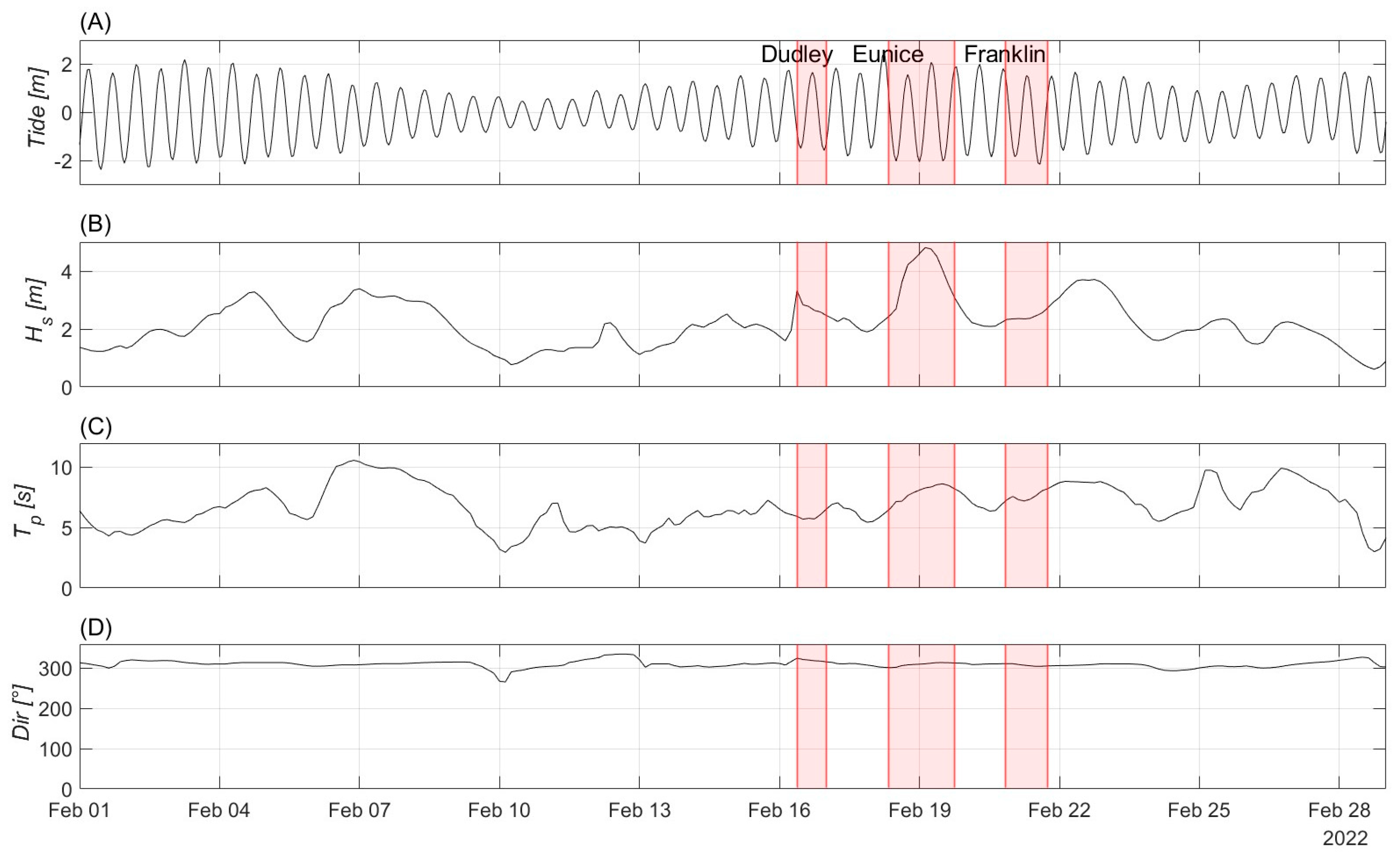
Figure 3.
(a) Overview of Brandon Bay with the location of both cameras; (b) detail of the field of view of Camera 1, represented by the yellow triangle; and (c) detail of the field of view of Camera 2, on a satellite image (from ESA—Sentinel 2).
Figure 3.
(a) Overview of Brandon Bay with the location of both cameras; (b) detail of the field of view of Camera 1, represented by the yellow triangle; and (c) detail of the field of view of Camera 2, on a satellite image (from ESA—Sentinel 2).
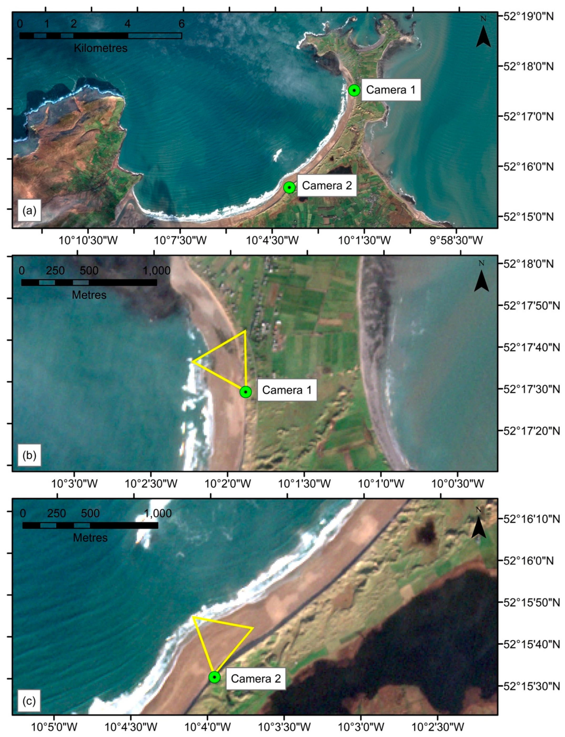
Figure 4.
Photo of Brinno TLC2000 Camera 1 deployed in the field.

Figure 5.
Road traffic cones were placed in the field and used as temporary GCPs.

Figure 6.
Temporary GCPs used in the field (Camera 2), with the red circles representing the GCPs.

Figure 7.
(A) Image taken by Camera 2 and (B) the same image after georectification.
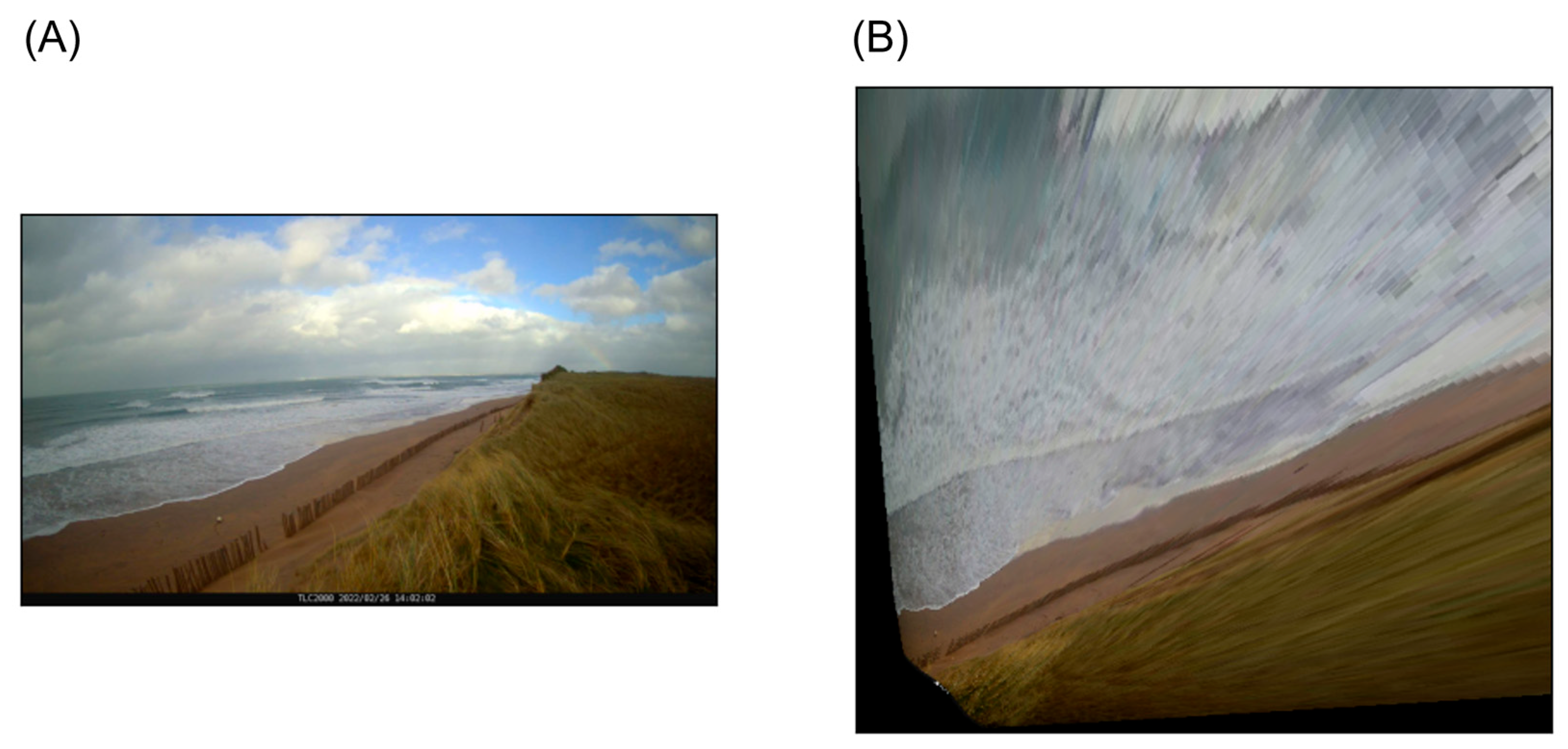
Figure 8.
Transects covering the swash zone in front of Camera 2 (From 26 February 2022)—interval 1 s. The blue line is the detected shoreline.
Figure 8.
Transects covering the swash zone in front of Camera 2 (From 26 February 2022)—interval 1 s. The blue line is the detected shoreline.

Figure 9.
Flowchart detailing the methodology.
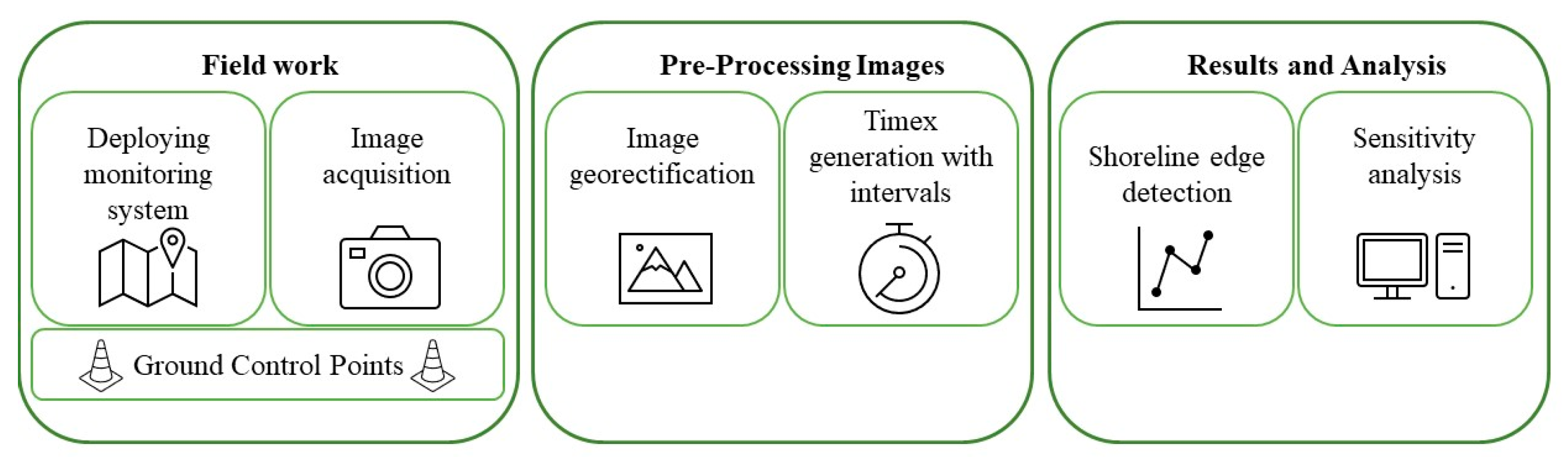
Figure 10.
Example of the shoreline edge (in blue) at different intervals on 26 February 2022 at high tide, with the shoreline edge at (a) 1 s, (b) 3 s, (c) 5 s, (d) 10 s, (e) 20 s, and (f) 30 s.
Figure 10.
Example of the shoreline edge (in blue) at different intervals on 26 February 2022 at high tide, with the shoreline edge at (a) 1 s, (b) 3 s, (c) 5 s, (d) 10 s, (e) 20 s, and (f) 30 s.

Figure 11.
Example of RMSD between shoreline edge detected on Timex with 1 s interval (solid line) and 5 s interval (dashed line) from 26 February 2022 at high tide. The red area represents the RMSD between both lines.
Figure 11.
Example of RMSD between shoreline edge detected on Timex with 1 s interval (solid line) and 5 s interval (dashed line) from 26 February 2022 at high tide. The red area represents the RMSD between both lines.

Figure 12.
Mean RMSD (solid blue line) and standard deviation (shaded areas) of all intervals compared to the 1 s interval of the different daylight hours, for (Top) Camera 1 and (Bottom) Camera 2, based on 796 Timex images.
Figure 12.
Mean RMSD (solid blue line) and standard deviation (shaded areas) of all intervals compared to the 1 s interval of the different daylight hours, for (Top) Camera 1 and (Bottom) Camera 2, based on 796 Timex images.

Figure 13.
Example of (A) snapshot and (B) resulting Timex image during receding tides, showing remaining water on the beach face resulting in shoreline edge detection not representing the actual shoreline (from 26 February 2022 at 10 h).
Figure 13.
Example of (A) snapshot and (B) resulting Timex image during receding tides, showing remaining water on the beach face resulting in shoreline edge detection not representing the actual shoreline (from 26 February 2022 at 10 h).

Figure 14.
Mean RMSD (solid blue line) and standard deviation (shaded areas), for intervals of 3 s, 5 s, 10 s, 20 s, and 30 s, compared to 1 s interval, for (Top) Camera 1 and (Bottom) Camera 2.
Figure 14.
Mean RMSD (solid blue line) and standard deviation (shaded areas), for intervals of 3 s, 5 s, 10 s, 20 s, and 30 s, compared to 1 s interval, for (Top) Camera 1 and (Bottom) Camera 2.
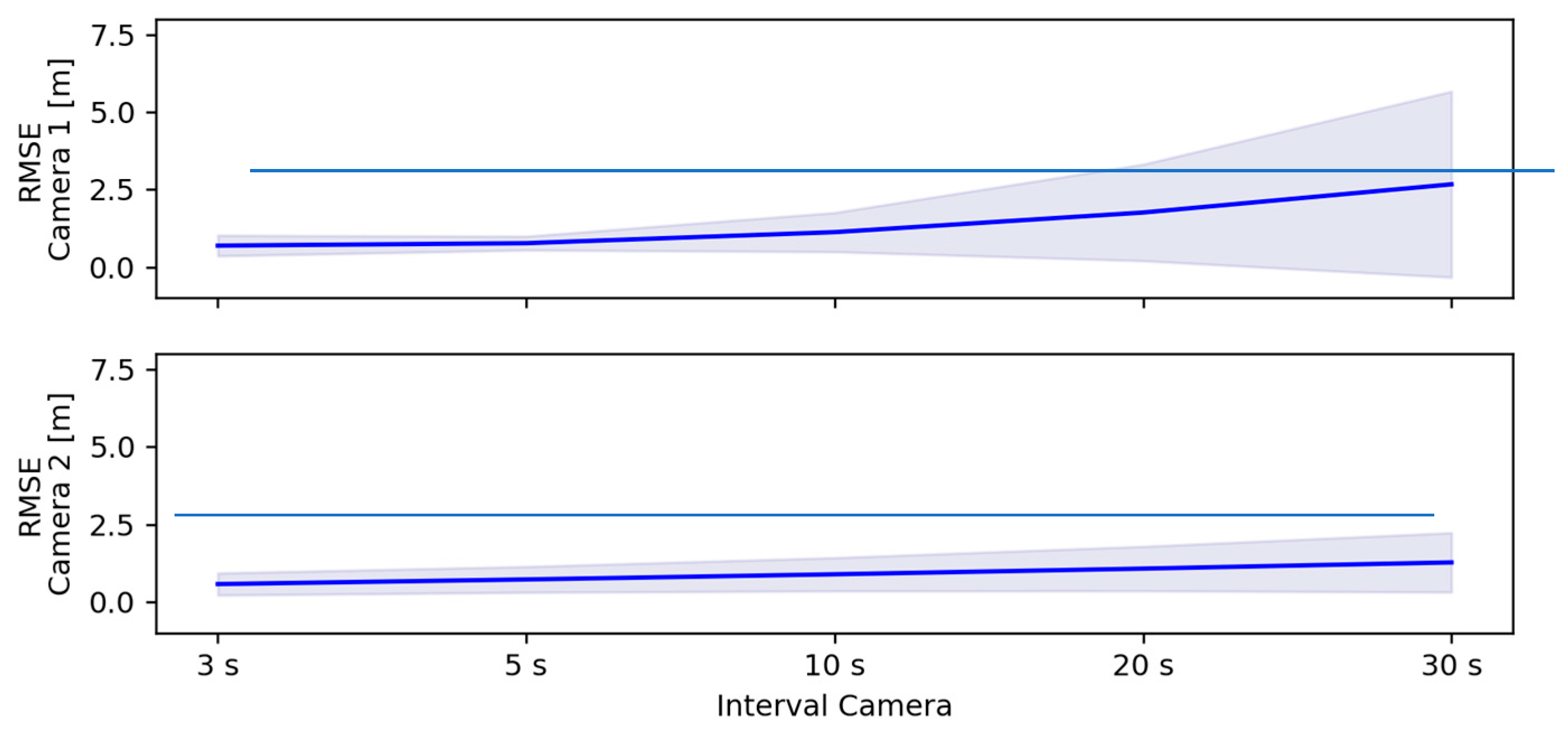
Figure 15.
(A) Average battery life for the different intervals, and (B) average days that SD card can be used for the different intervals, from Brinno (2022).
Figure 15.
(A) Average battery life for the different intervals, and (B) average days that SD card can be used for the different intervals, from Brinno (2022).


Table 1.
Overview of the cameras deployed in Brandon Bay.
| Site | Location ITM [m] | Camera Specifications | Elevation ITM [m] | FoV [m] | ||||
|---|---|---|---|---|---|---|---|---|
| Easting (Latitude) | Northing (Longitude) | Type | Pixel Resolution | Battery | SD Card | |||
| 1 | 458,967.02 (52°15′31.08″) | 613,891.61 (−10°3′57.41″) | Brinno TLC 2000 | 1980 × 1080 | 16 × AA | 128 GB | 11 | 200 |
| 2 | 461,425.81 (52°17′28.31″) | 617,447.31 (−10°1′53.09″) | 14 | 250 | ||||
Table 2.
Overview of intervals analysed in this study.
| Overview Intervals | |||
|---|---|---|---|
| Interval [s] | Time Period [min] | Total Images | Memory Demand [MB] |
| 1 | 10 | 600 | 93.3 |
| 3 | 10 | 200 | 31.2 |
| 5 | 10 | 120 | 18.7 |
| 10 | 10 | 60 | 9.5 |
| 20 | 10 | 30 | 4.8 |
| 30 | 10 | 20 | 3.2 |
Table 3.
Details on Timex images used for analysis.
| Total Number of Accepted Timex Images | ||
|---|---|---|
| Hour | Camera 1 | Camera 2 |
| 0—Low tide | 12 | 12 |
| 1 | 12 | 36 |
| 2 | 24 | 24 |
| 3 | 24 | 36 |
| 4 | 24 | 42 |
| 5 | 36 | 42 |
| 6—High tide | 36 | 42 |
| 7 | 36 | 42 |
| 8 | 36 | 38 |
| 9 | 36 | 42 |
| 10 | 36 | 32 |
| 11 | 24 | 36 |
| 12—Low tide | 12 | 24 |
| Total | 348 | 448 |
Table 4.
Comparison of results with previous studies.
| Study | Camera Type | Sampling Rate | Method | Camera Elevation [m] | FoV [m] | RMSD [m] |
|---|---|---|---|---|---|---|
| This study | Brinno TLC2000 | 10 min at 1 Hz | Red minus blue channel | 11 and 14 | Camera 1:
| 1.4 0.9 |
| [51] | Surfcam | 10 min at 5 Hz | Pixel intensity | 80 | Alongshore: 800 Cross-shore: 400 | / |
| [61] | / | 10 min at 2 Hz | / | / | Alongshore: 100 Cross-shore: 16 | 1.41 |
| [59] | ARGUS | 10 min at 2 Hz | ASLIM method | 43 | Alongshore: 1500 Cross-shore:120 | 5.1 |
| [64] | Bullet cameras | Averaged over short periods (30 s) | Colour contrast between water and beach | 11 | Alongshore: 1340 | 0.93 |
| [62] | Point Gray Blackfly 5 MP | 900 video frames at 1.5 Hz | Four methods:
| 15.9 | Alongshore: 250 Cross-shore: 112 | 1.71 |
| [65] | Mobotix M22 | 10 min at 1 Hz | ANN | 20 | Alongshore: 700 Cross-shore: 200 | 1.06 |
Disclaimer/Publisher’s Note: The statements, opinions and data contained in all publications are solely those of the individual author(s) and contributor(s) and not of MDPI and/or the editor(s). MDPI and/or the editor(s) disclaim responsibility for any injury to people or property resulting from any ideas, methods, instructions or products referred to in the content. |
© 2024 by the authors. Licensee MDPI, Basel, Switzerland. This article is an open access article distributed under the terms and conditions of the Creative Commons Attribution (CC BY) license (https://creativecommons.org/licenses/by/4.0/).
Share and Cite
MDPI and ACS Style
Nuyts, S.; Farrell, E.J.; Fennell, S.; Nash, S. An Assessment of the Role of the Timex Sampling Strategy on the Precision of Shoreline Detection Analysis. Coasts 2024, 4, 347-365. https://doi.org/10.3390/coasts4020018
AMA Style
Nuyts S, Farrell EJ, Fennell S, Nash S. An Assessment of the Role of the Timex Sampling Strategy on the Precision of Shoreline Detection Analysis. Coasts. 2024; 4(2):347-365. https://doi.org/10.3390/coasts4020018
Chicago/Turabian StyleNuyts, Siegmund, Eugene J. Farrell, Sheena Fennell, and Stephen Nash. 2024. "An Assessment of the Role of the Timex Sampling Strategy on the Precision of Shoreline Detection Analysis" Coasts 4, no. 2: 347-365. https://doi.org/10.3390/coasts4020018