Article

Policy Assessment for Energy Transition to Zero- and Low-Emission Technologies in Pickup Trucks: Evidence from Mexico

by
Julieth Stefany Garcia
1,
Laura Milena Cárdenas
2,
Jose Daniel Morcillo
3,* and
Carlos Jaime Franco
1
1
Facultad de Minas, Universidad Nacional de Colombia, Medellín 050034, Colombia
2
Facultad de Ingeniería, Universidad de Antioquia, Medellín 050010, Colombia
3
Facultad de Ingeniería y Tecnologías, Universidad de Monterrey, Monterrey 66238, Mexico
*
Author to whom correspondence should be addressed.
Energies 2024, 17(10), 2386; https://doi.org/10.3390/en17102386
Submission received: 29 February 2024 / Revised: 3 May 2024 / Accepted: 10 May 2024 / Published: 15 May 2024

Abstract

:
The transport sector is under scrutiny because of its significant greenhouse gas emissions. Essential strategies, particularly the adoption of zero- and low-emission vehicles powered by electricity, are crucial for mitigating emissions in road transport. Pickups, which are integral to Mexico’s fleet, contribute to such emissions. Thus, implementing effective policies targeting pickups is vital for reducing air pollution and aligning with Mexico’s decarbonization objectives. This paper presents a simulation model based on system dynamics to represent the adoption process of zero- and low-emission vehicles, with a focus on pickups and utilizing data from the Mexican case. Three policy evaluation scenarios are proposed based on the simulation model: business as usual; disincentives for zero- and low-emission vehicles; and incentives for unconventional vehicles. One of the most significant findings from this study is that even in a scenario with a greater number of vehicles in circulation, if the technology is fully electric, the environmental impact in terms of emissions is lower. Additionally, a comprehensive sensitivity analysis spanning a wide spectrum is undertaken through an extensive computational process, yielding multiple policy scenarios. The analysis indicates that to achieve a maximal reduction in the country’s emissions, promoting solely hybrid electric vehicles and plug-in hybrid electric vehicles is advisable, whereas internal combustion engines, vehicular natural gas, and battery electric vehicles should be discouraged.

1. Introduction

The transportation sector has emerged as a focal point, given its pronounced contribution to greenhouse gas emissions [1,2,3,4]. Strategic measures endorsed within the transportation sector encompass sustainable biofuels, low-emission hydrogen, and their derivatives, exhibiting potential for mitigating CO2 emissions generated from maritime, aviation, and land freight transportation [5]. Some of these implemented measures are related to more efficient public transportation systems, the development of biofuels and synthetic fuels, the use of hydrogen in the sector, and active mobility initiatives. However, the extensively embraced strategies are zero- and low-emission vehicles powered by low-greenhouse gas emission electricity, demonstrating significant potential for reducing greenhouse gas emissions throughout the life cycle of land-based transportation [6,7].
Mexico’s behavior is not significantly different from global patterns. According to the National Inventory of Emissions of Greenhouse Gases and Compounds for the years 2020–2021, which presents estimates of emissions and absorption of greenhouse gases and compounds, Mexico emitted 714,047 Gg of CO2e as of 2021. Of this total, 62.3% (444,592 Gg of CO2e) is attributed to the energy sector. Additionally, the transportation sector accounts for 20.7% of the overall CO2 emissions (148,043 Gg of CO2e), with road transportation representing 94% of this sector’s contribution (139,154 Gg of CO2e) [8]. According to the National Institute of Statistics and Geography (INEGI by its Spanish initials), in 2019, Mexico boasted a vehicular fleet totaling 47,790,950 vehicles, as officially registered by state and municipal authorities. This fleet includes 32,291,454 automobiles, 437,412 passenger trucks, 10,978,662 cargo trucks (including pickups), and 4,083,422 motorcycles, as shown in Figure 1.
Concerning zero- and low-emission technologies, data from the INEGI reveal that in 2016, there were 8265 electric and hybrid vehicles (battery electric vehicles (BEVs), plug-in hybrid electric vehicles (PHEVs), and hybrid electric vehicles (HEVs)), constituting 0.5% of the total sales for that year. However, by 2019, registrations surged to 25,608, representing 1.9% of the overall sales, indicating a noteworthy 1.4% increment. For 2022, a total of 45,249 electric and hybrid vehicles were registered.
Pickup trucks hold a pivotal role in the automotive landscape of Mexico. For instance, between January 2019 and December 2022, the growth rate averaged at 0.112%. However, from January to December 2023, the monthly growth rate surged to an average of 6.60% [9]. This notable increase underscores the segment’s importance in evaluating the energy transition process, given that, as it has a greater share in the total fleet, this segment consumes more energy and generates more emissions. Moreover, when analyzing emissions from the pickup segment within the 2025 framework, the technology pathways of EPA demonstrate an average emission factor of 160 gCO2/km within a footprint range of 70–80 m2 [10].
To mitigate emissions from the road transport sector in Mexico, a set of penetration targets for electric technologies have been proposed, as outlined in current public policy documents. Although the country’s goal by 2030 is for 50% of light and heavy vehicles linked to the national fleet to have zero emissions, this shows that it is necessary to work to promote replacement processes and thus reduce emissions from the transport sector.
In the context of Mexico, two noteworthy studies contribute to the understanding of this country’s transition to low-emission vehicles. First, a comprehensive analysis [11] was performed to investigate transformations within privately owned vehicle fleets, exploring the fiscal implications of introducing BEVs through a diffusion model. Although this study did not explicitly focus on pickup trucks, it highlighted the importance of policy implementation in encouraging the widespread adoption of zero- and low-emission technologies. Second, another study [12] examined the broader energy transition for vehicles in Mexico through a detailed multivariate analysis of economic and ecological factors influencing the procurement of low-emission vehicles. The findings emphasized a positive correlation between adopting sustainable practices and the acquisition of such vehicles in Mexico, with an emphasis on the consumer preference for affordability over energy efficiency considerations.
Other studies focused on pickup trucks in Mexico [13,14]. However, the significance of these studies lies in their exploration of last-mile logistics for these vehicles and the challenges posed by the availability of a recharging infrastructure. One study [13] investigated “last-mile” logistics by addressing the EV routing problem with simultaneous pickups, deliveries, and time windows from a multi-objective distribution perspective [13]. Meanwhile, another study [14] addressed the EV routing problem within the context of the pickup and delivery problem with time windows. Furthermore, computational experiments assessed the solution quality of the proposed approach [14].
Studying public policy plans to promote zero- and low-emission pickups is essential for distinct reasons. First, pickups represent a substantial portion (2%) of the vehicle fleet. Given their contribution to pollutant emissions, implementing effective policies can directly reduce air pollution and improve air quality. Additionally, considering the growing environmental awareness and need to address climate change, encouraging the use of low-emission technologies in pickups can significantly contribute to Mexico’s decarbonization goals. Analyzing policies also allows us to understand how incentives and taxes can influence consumer behavior, promoting the adoption of cleaner and more sustainable vehicles. Ultimately, comprehensively assessing public policies aimed at promoting zero- and low-emission pickups is crucial for advancing towards cleaner and more competitive mobility.
During this literature review process, we identified a lack of research specifically focusing on the pickup segment to assess various policies related to their incentives and taxes and their impact on emissions in the transportation sector. This represents a pertinent subject for decision-making and meeting national commitments. Following the above, and given the importance of the pickup segment in the total vehicle fleet of Mexico and to implement the analysis in a vehicle category, this study aimed to evaluate the energy policy for the transition towards zero- and low-emission technologies in pickups in Mexico using system dynamics as the modeling methodology and a broader spectrum sensitivity analysis from a computational model that allows visualization based on a set of defined parameters, enabling the identification of the ideal scenario for achieving the decarbonization of the transportation sector.
In Latin America, we find ourselves lagging behind in the decarbonization of the transport sector compared with other countries [2,15]. Therefore, implementing our model can be beneficial for Latin American countries as it provides tools that help evaluate their energy transition processes more efficiently and effectively. The need for comprehensive evaluations is imperative, as the complexity of these processes does not allow for ad hoc experimentation with policy evaluation [16]. Consequently, there must be computational tools for preventing the loss of time due to the hasty implementation of policies and enabling a more informed anticipation of potential societal repercussions [6,17]. These tools not only complement ongoing efforts but also provide clarity and guidance to countries that are advancing more slowly in the development and implementation of policies during the transition towards zero- and low-emission technologies [16,18].
We structured the remainder of this paper as follows: In Section 2, we provide the theoretical and political frameworks for EVs in Mexico. Section 3 outlines the materials and methods utilized. Section 4 presents the results of simulations derived from the modeling process and the broader spectrum sensitivity analysis. In Section 5, we analyzed the outcomes of each modeled scenario. Finally, in Section 6, we present our conclusions and suggest potential avenues for future research.

2. Theoretical and Political Frameworks of EVs in Mexico

Mexico is keen on promoting electric and hybrid technologies across the nation. This commitment is reflected in the regulation of the National Electric Mobility Strategy (Estrategia Nacional de Movilidad Eléctrica by its Spanish initials), which seeks to establish foundational principles and guidelines on environmental, technical, technological, financial, legal, institutional, and administrative aspects. The overarching goal is to position electric mobility as a viable and sustainable alternative on a national scale, effectively contributing to the reduction in greenhouse gas emissions and pollutants [19].
In pursuit of decarbonization and the widespread adoption of sustainable technologies, Mexico’s National Electric Mobility Strategy (ENME by its Spanish initials) established ambitious goals for the years 2030, 2040, and 2050. By 2030, 50% of sales of both light and heavy-duty vehicles are projected to be zero-emission units, contributing to an accumulated reduction of 30 million tons of carbon dioxide equivalent (MtCO2e). Goals include the integration of EVs into the public transport systems of the ten most polluted cities and the development of a public electric charging infrastructure nationwide [19]. By 2040, 100% of vehicle sales are expected to be electric and plug-in hybrid, with an accumulated reduction of 129 MtCO2e. Additionally, plans include having sufficient charging systems in both cities and federal highways. Finally, for 2050, the aspiration is for all vehicle sales to be electric, with an accumulated reduction of 272 MtCO2e [19]. Furthermore, a consolidated electric system for heavy-duty vehicles is to be established on the country’s strategic roads. These goals reflect Mexico’s commitment to transitioning towards more sustainable mobility and mitigating emissions [19].
This strategy seeks to facilitate the incorporation of EVs into freight transportation, aiming to achieve its objectives by 2030, primarily focusing on emission reduction in key commercial freight corridors [19]. Recognizing the substantial contribution from diesel-powered freight fleets to the nation’s overall emissions, a range of measures have been proposed for implementation in the short, medium, and long term. These encompass formalizing freight transport companies, providing fiscal incentives to encourage the adoption of EVs, promoting sustainable business models, and instituting comprehensive training programs across the sector for electric mobility. Furthermore, robust advocacy is in place for the implementation of more stringent safety and energy efficiency regulations. Simultaneously, there is a clear commitment to actively promoting the electrification of commercial routes and embracing long-term mobility models centered around hydrogen.
Furthermore, in Mexico, advancements in electric mobility have been facilitated, among other initiatives, through governmental schemes that incentivize the adoption of zero- and low-emission technologies. The Mexican government issued a decree emphasizing the benefits associated with the use of EVs, addressing aspects such as income tax, value-added tax legislation, the federal tax code, and the law on taxes for new vehicles, with the latter being the primary incentive.
Some of the regulated incentives in Mexico include the following [19]:
  • Exemption from the New Vehicle Tax: EVs are exempt from paying this tax.
  • Exemption from tenancy payments: In most states, EVs are exempt from paying tenancy. In the State of Mexico, no tenancy is paid during the first 5 years; afterward, a 50% discount applies.
  • Exemption from environmental verification: Due to the nonpolluting technologies used in their propulsion, EVs are exempt from the vehicle verification program, which involves semiannual emission inspections and the restriction of the Hoy No Circula program.
  • Elimination of tariffs: Tariffs are eliminated for the importation of vehicles with electric motors, including cars, vans, and cargo trucks. This applies to companies subscribed to the decree for competitiveness support, as proposed by the Ministry of Economy.
  • Deductibility of the income tax for the acquisition of charging stations: According to the General Criteria for Economic Policy for the Income Law Initiative and the Federal Budget Project for the Fiscal Year 2017, a tax credit is established to deduct 30% of the income tax for the public-access EV charging infrastructure.

3. Materials and Methods

3.1. System Dynamics

The system dynamics methodology was selected for modeling in this study owing to its ability to facilitate the replication and comprehension of dynamics in social behavior, anticipate future system conditions, and analyze the effectiveness of strategies and policies in simulated environments. With a dedicated focus on the analysis of technological diffusion and policy evaluation, system dynamics distinguishes itself from other methodologies by capturing elements such as feedback, complexity, delays, and nonlinearities [20,21]. Several previous studies have utilized system dynamics to evaluate public policies in the transportation sector [1,22,23,24,25,26].
Drawing upon this methodology, we built a simulation model to assess the behavior of public policies implemented in the widespread adoption of zero- and low-emission pickup trucks, with Mexico serving as a case study. This process encompassed not only the construction of the model per se but also a thorough analysis and characterization of the resulting dynamics, adhering closely to the methodological guidelines articulated previously [20]. In the subsequent formulation of the simulation model, we represented both the structure and decision rules, conducted parameter estimations, and established the initial conditions of our variables. A coherence test was then administered to ensure alignment with the predetermined objectives and limitations. Culminating this phase, a series of tests were executed, incorporating comparisons with empirical data or external benchmarks, assessments of robustness under extreme conditions, and an exploration of the model’s sensitivity to diverse scenarios. Within the modeling process, various technologies were considered, such as BEVs, PHEVs, HEVs, internal combustion engines (ICEs), and vehicular natural gases (VNGs).

3.2. Model Structure

In this excerpt from our paper, we intend to present the overall structure of the model developed using system dynamics. Given the model’s complexity, the complete structure and detailed equations can be found in Appendix A, offering a more robust insight into the information. Here, we provide a modular representation of the model to introduce its general structure.
In Module ❶, a discrete choice model was developed as an integral component of the system dynamics modeling methodology. The conceptual framework for constructing this discrete choice model was based on the seminal contributions from a previous study [25]. In adherence to the authors’ methodology, a comprehensive set of five pivotal attributes was identified in the decision-making process for electric technologies [25]. These include vehicle price, autonomy, tax considerations, energy cost, and charging infrastructure accessibility. Furthermore, the model was calibrated in VENSIM (version 10.1.2) software using previously elucidated coefficients [25]. This discrete choice model enables utility values to be assigned to each vehicular technology and facilitates the discernment of the probability associated with selecting each technological option. Such probabilities, in turn, directly affect the observed upswing in vehicle sales associated with each distinct technology.
In Module ❷, the modeling of fleet behavior was conducted by integrating the buyer’s probability of choice, thereby exerting an impact on the sale trajectories of individual technologies. This analytical framework considered all pickup trucks, including potential replacements at the end of their operational lives, and considered the increase in vehicle quantity due to dynamic demographic trends in Mexico.
The pickups’ x change over time, given in [ p i c k u p s ] , is the difference between pickups entering the market ( P I ) and those leaving the market ( P O ). Each technology considered (BEVs, ICEs, VNGs, HEVs, and PHEVs) replicates this structure. Thus, the state equations are defined as follows:
d x d t = P I P O
The entry of pickups into the market ( B I ) depends on the following factors: a probability of choice resulting from the discrete choice model λ given in % and the total sales T S given in [ p i c k u p s ] .
P I =   λ · T S
The exiting pickup depends on x , and the fleet’s lifespan relies on μ , given in y e a r .
P O =   x μ
In Module ❸, due consideration was given to the fleet growth outcomes obtained from Module ❷, specifically those regarding BEVs, PHEVs, and HEVs. This consideration aimed to model the requisite charging infrastructure essential for meeting the evolving demands of the EV system. Subsequently, Module ❹ incorporated the number of pickups identified in Module ❷ to calculate the capital expenditure (CAPEX) indispensable for procuring a technology aligned with each energy source. This module distinguishes between variable CAPEX, which is contingent upon nationally implemented incentives and policies, and constant CAPEX, which is exclusively grounded in the prevailing market value of vehicles. Notably, we integrated the acquisition cost of the infrastructure for technologies that require electric charging, such as BEVs and PHEVs. Note that regarding the variable CAPEX, a series of learning curves were constructed based on market research and the review of price projections published by Bloomberg [27].
Culminating the systematic modeling, Module ❺ executed a computation of emissions emanating from the fleet operations delineated in Module ❷. This assessment encompassed emission factors associated with gasoline and VNGs. Additionally, considerations extended to the activity factor, reflecting the annual mileage for each vehicle alongside the average efficiency for ICEs and VNGs.
We accumulated emissions from the operation of a diesel fleet and a VNG fleet. This analysis was based on a tank-to-wheel approach [28], focusing solely on the operational emissions generated by the fleet while disregarding emissions associated with the complete lifecycle of the vehicles. The accumulated gasoline emissions C E I C E , given in K g C O 2 , represent the emissions resulting from the operation of the gasoline fleet over time, which we denoted as I C E E , given in T o n C O 2 / y e a r . Similarly, the accumulated VNG emissions C E V N G , given in K g C O 2 , represent the emissions resulting from the operation of the natural gas fleet over time, which we denoted as V N G E , given in T o n C O 2 / y e a r .
d C E I C E d t 1000 = I C E E
d C E V N G d t 1000 = V N G E
We calculated the gasoline and VNG emissions by considering the number of vehicles, x , the average kilometers traveled per vehicle, A , the emission factor, E F   [29], and the fuel economy, F E , per technology.
C E I C E = x I C E · A I C E F E I C E · E F I C E
C E V N G = x V N G · A V N G F E V N G · E F V N G
The general structure of the model is shown in Figure 2.

3.3. Model Validation and Input Data

As part of the model validation process, we conducted several tests to validate the structure and parameters of the model, as outlined previously [30]. To confirm the theoretical structure of the proposed model, we reviewed the pertinent literature to establish causal relationships. Throughout the model’s development phase, we verified its theoretical parameters by defining their applicable ranges, as mentioned earlier. Evidence of the parameter confirmation test is presented in Table 1, which displays the essential model parameters, their corresponding values, units of measurement, and information sources. Furthermore, the accuracy of the proposed units was verified by conducting a dimensional consistency test, as stated in [21,31]. Additionally, we performed extreme value tests to assess the limitations and scope of the model, as indicated in [31]. Table 1 presents the model’s main parameters, and Appendix A provides the complete documentation of the model and other data used for its calibration.
For model calibration, various data sources were employed. To gather information on vehicles in circulation up to 2023, two databases were utilized. The first database used was the open database provided by the National Institute of Statistics and Geography (INEGI) [9], from which data on the annual fleet in operation from 1991 to 2023 for ICE, VNG, and HEV technologies were filtered from [32]. The second source used was the subscription-based database EV volumes [33], which contain global information on the quantity of sold electric and plug-in vehicles. For model development, pre-existing data from this database from 2010 to 2023 were utilized.
Additionally, the website Autocosmos was utilized as another source to calibrate the model [34,35]. Autocosmos serves as a platform that consolidates vehicle prices in Mexico, offering detailed information on various types of vehicles and fuels. Owing to its regular updates on purchase prices, this platform proved to be a suitable resource for our research.
Furthermore, regarding assumptions related to the activity factor, emission factor, and fuel economy for each technology, data from the emission inventory of Bogotá for the year 2020 were employed [29]. This was based on the inventory’s status as the most current and relevant information applicable to Latin American countries. This emission inventory provides updated data for 2020 from various sources, encompassing mobile sources on roads, emissions from dust resuspension on roads, as well as brake and tire wear. To estimate emissions from mobile sources, a diverse range of data sources was utilized, including real-world operational measurements supplemented by internationally recognized values and recent local studies conducted in Latin American cities [29]. This approach was chosen due to potential similarities in fleet operations among Latin American cities compared with those on other continents.
Additionally, to validate our model and explore a broader spectrum of scenarios, we conducted an extensive computational exercise in Section 4.5. This experiment scrutinized our model for illogical behaviors and yielded numerous possible outcomes when various combinations of policies or parameter values were adopted.

3.4. Simulation Scenarios

During scenario construction, we considered decision criteria. The initial scenario, “Business as Usual” (BAU), reflects the existing regulatory landscape of policies and incentives, as presented in Section 4.1 The second scenario, “No Transition”, represents the absence of incentives and the existence of similar taxes for all technologies, establishing uniform conditions for all technologies. Finally, the third scenario, “New Incentives”, introduces a robust fortification of incentives, resulting in discernibly diminished purchase and operational costs for pickup trucks. Table 2 presents the values underpinning each scenario, providing a representation of the considerations made in this scenario analysis.
The presented information reflects the percentage of charges the vehicle owner must bear for the purchase, ownership, or incentive. For example, the 3% operating fee for ICE and VNG technologies means the owner must pay 3% of the initial vehicle value to operate it. In the case of incentives, for example, the 20% value in the New Incentives scenario corresponds to a saving of this proportion in the vehicle purchase price.
On the basis of the assumptions outlined, the simulations presented in Section 3 were constructed.

4. Results

This section presents the results of the simulations. To enhance clarity, each simulation is presented in subsections. Additionally, this section presents the results from the broader spectrum sensitivity analysis and detailed outcomes derived from the developed computational model.

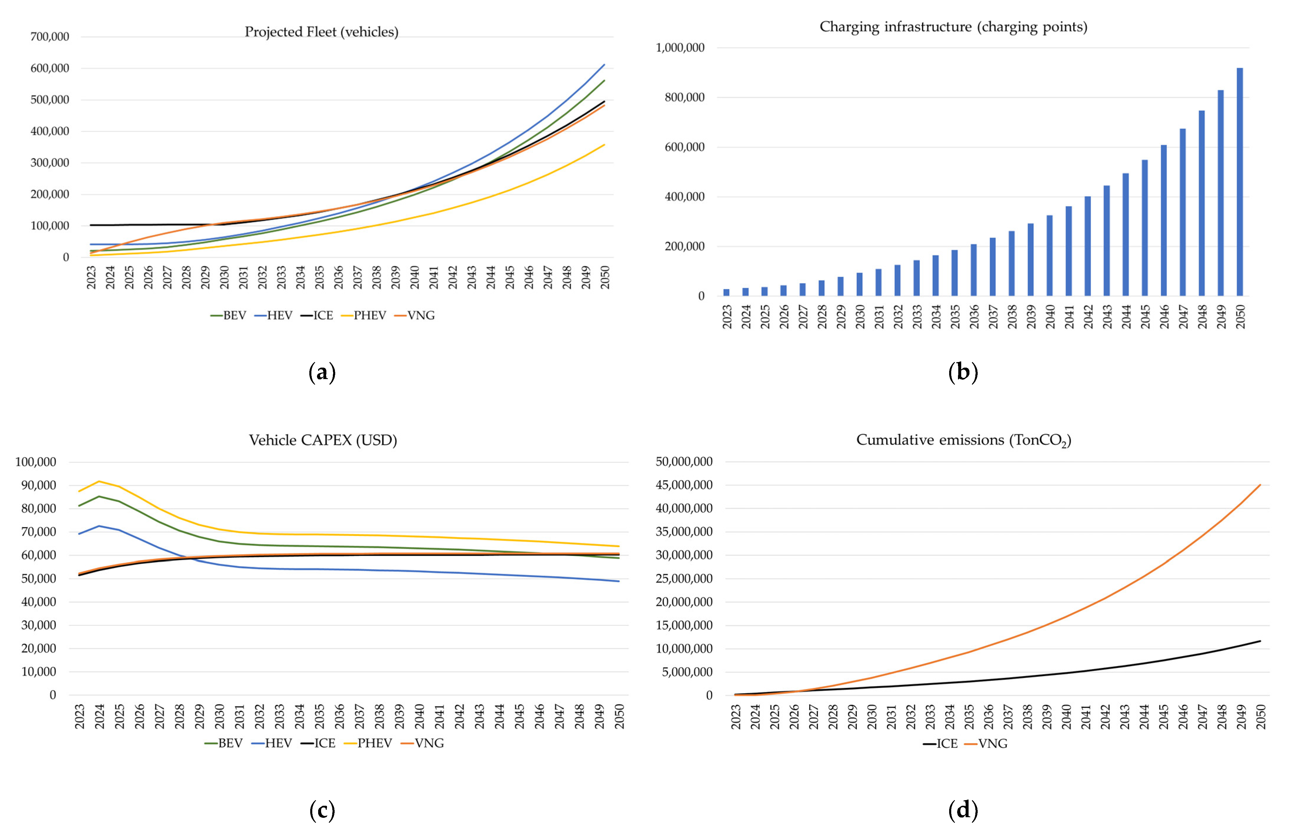
4.1. Business as Usual

Figure 3 presents the simulation results for the BAU scenario, representing four indicators considered relevant for evaluating current public policies implemented in Mexico. These indicators are the projected fleet by technology, the number of required charging points, the projected CAPEX by technology, and future emissions from remaining combustion technologies.
The simulations reveal that existing incentives and taxes in Mexico generate interest in zero-emission technologies among pickup users, given the substantial growth in BEVs. This is due to the 10% saving that buyers obtain in the initial vehicle value through the currently active incentive, a circumstance that also benefits HEVs. Notably, vehicle value is a relevant criterion in decision-making, creating a significant impetus for the growth of these technologies. Meanwhile, the growth of BEVs, HEVs, and PHEVs in 2026 is related to the anticipation of decreasing commercial and importation costs for these technologies in that year, driven by the dynamics and reductions in the prices of key cost components, such as the value of the battery. Consequently, this surge implies a greater need for charging points, estimated to reach close to 2 million chargers, assuming the installation of one charging point per vehicle.
In contrast, taxes currently applied to ICE and VNG technologies evidently tend to remain constant, aligned with market maturity. This differs from those applied to zero- and low-emission technologies, which show an upward trend over the next 3 years, followed by a subsequent decline. This pattern arises from the assumption that, as emerging technologies, their initial costs are higher compared with historically commercialized technologies. However, as the market becomes more dynamic and more manufacturers actively participate in the development of vehicles and batteries, and as technologies are optimized, competitive prices will be achieved in the future. Additionally, the 10% scenario’s influence on the initial value promotes cost reduction through incentives.
In the emission simulation, a noteworthy contribution of emissions from VNG vehicles is apparent, driven by their emission factor and participation in terms of vehicles.

4.2. No Transition

Figure 4 presents the simulation results for the No Transition scenario, representing four indicators considered relevant for evaluating nonexistent relevant public policies implemented in Mexico. In this scenario, we explored the long-term impact on the pickup truck fleet if no incentives were to promote energy transition in this vehicle category. The results revealed a significant growth in HEV technologies, attributed to their current cost, influenced by the importation from the United States, consumption efficiency, share in the overall fleet, and the learning curve of a robust technology compared with technology in a positioning phase. As shown in the graph, HEVs are the only technology type that achieved a lower CAPEX compared with combustion technologies, leading to rapid mass adoption.
Meanwhile, PHEV pickups exhibited the slowest growth, primarily due to their currently high technology cost. Without incentives, it will take some time for their commercial value to decrease. However, this reduction is expected to occur gradually, driven by increased stakeholder participation in commercial dynamics, which contributes to decreasing their value.
In this scenario, with the reduced participation of BEV technologies, there is an estimated need for around 900,000 charging points. In the emission analysis, VNG technology continued to dominate. This result sparks significant curiosity because, although it is not the technology with the highest number of vehicles, being commonly used in pickup trucks, it requires more torque for movement. This leads to higher natural gas consumption per kilometer traveled. In this case, although the emission factor of VNGs is lower than that of ICEs, their gas consumption is higher, reflecting their predominance in emissions.

4.3. New Incentives

Figure 5 presents the simulation results for the New Incentives scenario, showcasing the defined indicators. This scenario aimed to assess the system’s behavior under public policy actions promoting the deployment of zero- and low-emission technologies through stronger incentives and taxes for ICE and VNG vehicles. The details of these policies are presented in Table 2.
With the implementation of incentives, a significant growth of BEV pickups is evident, reaching around 3.4 million, followed by PHEVs and HEVs, both considered low-emission technologies. Similarly, the regulation of taxes that increases the costs of owning and operating ICE and VNG vehicles results in a rapid decline in sales.
Meanwhile, the high level of participation of battery technologies highlights a growing and significant need for charging points, which could become a potential constraint in the future.
Concerning CAPEX, with incentives generated for the purchase of zero- and low-emission technologies, a decrease in the purchase value is evident in the next 2 years. Notably, PHEV technology remains below the value of combustion technologies.
Finally, a high quantity of emissions is evident in BEVs, directly related to the number of vehicles, followed by emissions from the remaining ICE vehicles still participating in the overall fleet.

4.4. Scenario Comparison

In this section, we compare three simulated scenarios for two variables considered relevant: the projected total fleet and the projected emissions, view Figure 6. This is deemed one of our most significant findings as it illustrates that, in the absence of promoting policy actions supporting zero- and low-emission technologies, the long-term quantity of pickups is lower. When incentives are promoted, there is likely a heightened interest exhibited by vehicle buyers, given that the cost of the vehicle plays a crucial role in the discrete choice model. If the buyer perceives the technology as being more accessible, it results in an increased interest in vehicle ownership. Therefore, as BEVs become more affordable, the sale of more units is anticipated. This observed trend is also reflected in the number of vehicles circulating in the New Incentives scenario. Notably, during the modeling process, the fleet’s behavior considered replacements and the introduction of new fleet entries influenced by population dynamics and a growth rate determined by the country’s motorization rate.
However, although the No Transition scenario showed the fewest number of vehicles in circulation, it reflected the highest level of CO2 emissions. This is attributed to the environmental impact of gasoline combustion in conventional vehicles.

4.5. Broader Spectrum Sensitivity Analysis

As previously demonstrated, our analysis solely encompassed three scenarios, offering a limited scope of investigation. However, recognizing the necessity for a more comprehensive understanding of potential scenarios conducive to optimal emission outcomes, we embarked upon the design of an expanded spectrum encompassing twelve pivotal parameters. Because of computational constraints, we could only execute computations for three scenarios per parameter, as delineated in Table 3. The range of variation for the parameters is crucial for comprehensively assessing the dynamics of the system. It allows for a thorough exploration of potential scenarios and their implications.
Evidently, considering twelve parameters with three potential values each (as per the variation step) results in a total of 312 = 531,441 simulation outcomes or potential scenarios. This significantly broadens the spectrum compared with the mere three scenarios presented in Section 4.1, Section 4.2, Section 4.3 and Section 4.4. Additionally, each scenario encompassed a simulation period spanning 29 years (from 2022 to 2050), generating 15,411,789 data points for each variable. Consequently, if we analyze around 13 variables, this translates to over 200 million data points in total.
After computing the 531,441 scenarios, our next step was to identify the best-case emission scenario among the 200 million data points for the ICE, BEV, and VNG technologies; the values of the only parameters modified to obtain the best case are shown in Table 4. This entailed identifying the minimum emission value achieved over the 29-year simulation period (2022–2050) across the entire spectrum of scenarios. The resultant minimum values obtained are as follows:
Min (ICE emissions) = 6,142,920 CO2
Min (BEV emissions) = 381,477.6 CO2
Min (VNG emissions) = 25,119.62 CO2
Subsequently, we filtered the scenarios that yielded the minimum values, resulting in the identification of 117 scenarios representing the best-case emission outcomes for ICE, BEV, and VNG technologies. Upon calculating the central tendency of the 12 parameter values corresponding to these 117 scenarios, we obtained the following:
Only the aforementioned 12 parameter values can achieve the best-case emission scenario for all the technologies. To analyze the system’s behavior under these optimal emission conditions comprehensively, we plotted the 117-time series depicting the evolution of the fleet and emissions for all technologies, as illustrated in Figure 7.
The simulations presented in Figure 7 showcase the behavior of the previously defined indicators for the best-case scenarios for ICE, BEV, and VNG emissions. In this case, BEV emissions were considered to assess the influence of the emission factor of the national interconnected system, given the significance of the electricity generation source. Figure 7a illustrates that the predominance of low-emission technologies rests on HEVs, with PHEV technologies as a secondary option, to minimize emissions from ICE, BEV, and VNG technologies.
Meanwhile, Figure 7b demonstrates that the cost of hybrid (HEVs and PHEVs) and battery (BEVs) technologies must be reduced to values below the market price of combustion technologies by 2030 to achieve a scenario where emissions from ICEs, VNGs, and BEVs remain at an optimal level. This has a direct influence on the buyer’s decision criterion, leading to the prevalence of low-emission vehicle purchases, which is reflected in the emission reduction observed in Figure 7c.
A closer look at Figure 7c shows that, although ICE emissions are present, they are much lower than those of the other scenarios, including the New Incentives scenario. This new scenario, identified through the broader spectrum sensitivity analysis methodology, demonstrates that the operation tax must be increased within the range of 24% to 30% on these technologies, and incentives must be implemented in the same ranges to maintain lower emissions in combustion technologies. This would allow a decision-maker to assume that the proportion of the cost of the technology to be replaced and the incentive for the technology to be promoted should be proportional.
Moreover, Figure 7d shows the behavior of charging stations for the scenario obtained from the broader spectrum sensitivity analysis, highlighting the demand for charging points for PHEV technologies, which is the predominant technology when stabilizing emissions from ICEs, VNGs, and BEVs. In this case, the result is significant, as it allows us to conclude that the deployment of charging infrastructure is crucial for emission mitigation.
Finally, the model showed optimal energy values; however, given that BEV emissions were considered, the model optimized the outcome to avoid deploying this technology on a large scale, aiming to present the best emission scenario. This is why it increased the cost of electricity, a result that allowed us to assume that if electricity in Mexico becomes more economical, a massive deployment of BEVs could be achieved, bringing the results closer to those presented in the New Incentives scenario.

5. Discussion

From the simulations conducted for each scenario, diverse outcomes were identified that illustrate the prospective behavior of the pickup truck fleet across various vehicle technologies. This encompasses variations in CAPEX resulting from policy actions, charging infrastructure requirements, and emission behavior stemming from the fleet’s growth.
In the BAU scenario, the current incentives and taxes in Mexico will drive the growth of electric pickups until 2050. Additionally, HEVs and BEVs will have a more substantial share compared with ICEs and PHEVs. This implies a significant need for charging points, posing a challenge to the country’s electrical sector and necessitating an increase in electricity generation capacity to meet the demand for this vehicle quantity. The simulation also revealed a decrease in the initial investment cost for BEVs, HEVs, and PHEVs. This reduction is associated with market dynamics in zero- and low-emission technologies, the involvement of new electric technology dealers, and the decreasing price of batteries for electricity storage due to global technological development. Notably, VNGs significantly contribute to CO2 emissions given their anticipated high market share due to their price, autonomy, and energy availability nationwide. Moreover, around 2047, emissions from BEVs are projected to surpass those from ICE vehicles, considering the expected number of circulating vehicles during that year.
In the No Transition scenario, a notable participation of HEVs is evident due to low policy actions, such as incentives and taxes. This benefits HEVs, making them more competitive in monetary terms, considering their greater autonomy and performance. Under these conditions, HEVs and BEVs garner more buyer interest because of the parameters related to energy costs and autonomy. Regarding CAPEX, only HEVs achieve a lower cost than combustion technologies like ICEs and VNGs, contributing to the increased adoption of HEV pickups. PHEVs consistently have higher initial costs than other technologies, making them less competitive nationally. In terms of emissions, VNGs have the highest emission potential in this scenario because of their energy consumption, followed by ICE vehicles, and, finally, BEVs, considering fleet participation and their emission factor of electricity, which is lower than that of gasoline.
In the New Incentives scenario, a significant growth in the number of BEV pickups is evident, suggesting that increased policy actions promote the penetration of zero-emission technologies in the national fleet. However, this raises a potential discussion point, as a higher number of electric technologies does not necessarily correlate directly with a reduction in greenhouse gas emissions. Some authors argue that one of the most relevant alternatives for decarbonizing the transportation sector is the implementation of efficient integrated mass transportation systems, which reduces the number of individual vehicles in the national fleet. Although replacing the current combustion fleet could contribute to decarbonization, exponential fleet growth could result in increased emissions from electricity generation to meet the demand for these vehicles. Additionally, it may lead to planning issues, traffic congestion, and resource overexploitation in EV manufacturing.
One of the most significant outcomes demonstrated in this study, as depicted in Figure 6, pertains to the comparison between the projected fleet and emissions across the three scenarios. This holds particular significance as it illustrates that, in the New Incentives scenario (where the electric fleet experiences a substantial increase in its projection to 2050), with a considerable number of vehicles entering operation, the emissions are notably lower than those in the No Transition scenario and marginally lower than the BAU scenario. This leads us to infer that, even with a considerable number of EVs operating on Mexico’s roads, this remains a pertinent measure in the process of decarbonizing the transportation sector. Consequently, the implementation of incentives and public policy actions fostering the transition to zero- and low-emission technologies directly contributes to this country’s emission reduction goal.
Another pertinent aspect when scrutinizing the obtained results is linked to factors such as the country’s installed capacity to meet the electricity demand stemming from the increasing number of electric pickup vehicles in operation. Moreover, unconventional renewable energy sources must be integrated into the country’s power grid to ensure clean electricity charging, enhance the emission factor, and mitigate the environmental impact of the transportation sector. This consideration gains significance, particularly considering the substantial contribution of energy generated by thermoelectric plants in the country.
Meanwhile, the development of computational models that can accurately represent the deployment of zero- and low-emission technologies is crucial for decision-making in controlled environments that mirror the criteria of potential technology buyers. This effort resulted in a lot of simulated scenarios generated through a sensitivity analysis using Python code. Accordingly, the parameter sets that would benefit the least emissions from ICEs and VNGs stood out, such as operation tax VNG at 30%, operation tax ICE at 24.61%, operation tax HEV and PHEV at 10%, operation tax BEV at 30%, ICE incentives at −19.23%, BEV incentives at 10%, VNG incentives at −30%, HEV incentives at 29.23%, PHEV incentives at 25.38%, and the electric cost per kWh at 0.3 cents per kWh and gasoline cost per gallon at 3 USD per gallon. These facilitated the identification of various public policy options and sets of parameters for policy actions. Decision-makers can utilize these findings to document public policy guidelines with simulation results, effectively mitigating the impact of uncertainty.
As a point of discussion, the significance of establishing policies for the proper disposal of waste from EVs, particularly those generated by batteries, is emphasized. Additionally, rigorous environmental management plans safeguarding resources affected by the exploration and exploitation process of minerals to produce these technologies must be formulated. This becomes paramount, given the anticipated high participation of EVs in Mexico’s future across all three scenarios.
Lastly, our results closely align with the findings presented in various analyzed cases, highlighting the imperative need to implement comprehensive policies to promote the adoption of zero- and low-emission vehicles. To reduce greenhouse gas emissions in the transportation sector, similar efforts are being made in Canada [36,37], Australia [38], and particularly México [39]. We concur with the critical importance of combining multiple policies to achieve considerable reductions in greenhouse gas emissions and meet sales targets for zero- and low-emission technologies [37,38,40]. However, we emphasize the need for transition policies that focus on objectives rather than specific technologies to achieve optimal results [41]. Additionally, we observe that BEVs are an option with a considerably lower greenhouse gas emission footprint than conventional vehicles, as previously noted [5] in the case of Iran.
Additionally, we recognize the critical importance of having an adequate charging infrastructure, as previously analyzed for Mexico [39], and implementing changes in vehicle prices to achieve sales targets for zero-emission technologies and reduce greenhouse gas emissions [42]. Our analysis, supported by a system dynamics model, reinforces the importance of understanding the behaviors of EVs, PHEVs, HEVs, ICEs, and VNG vehicles, EV charging demands, and the impacts of policies on the adoption of zero-emission vehicles, such as prices, taxes, and incentives, to guide future actions towards more sustainable and environmentally responsible mobility [43]. Finally, among the relevant results are those obtained with hybrid technologies, which prove to be an optimal alternative for Mexico, considering the market context because of its proximity to the United States, a result that agrees with previous findings [44].

6. Conclusions

This article emphasizes the critical roles of incentives, taxes, and policy measures in driving interest towards zero- and low-emission technologies, which shape key parameters that influence purchasing decisions in the pickup truck segment. This strategic approach facilitates a transition away from conventional combustion technologies, contributing to a broader energy shift within the sector. Acknowledging that decarbonization involves alternative approaches beyond technology promotion, such as advocating for efficient mass transit systems and reducing the reliance on private vehicles, the analysis demonstrates that both the replacement of combustion technologies and the swift integration of electric technologies significantly impact total CO2 emissions in Mexico’s unique context. Despite the limited share of renewable sources in Mexico’s electricity grid, this study highlights a considerable emission reduction potential from adopting fewer polluting technologies. Expanding unconventional renewable energy sources presents a promising avenue for enhancing the positive effects of the ongoing energy transition, particularly in the pickup truck segment. This study concludes by emphasizing the need for addressing environmental concerns related to mineral extraction, vehicle manufacturing, and waste disposal, pointing to potential areas for future research that hold significant importance for decision-makers in Mexico.
One of the main challenges in obtaining a broader spectrum of sensitivity scenarios was computational capacity. We could only simulate three possible scenarios per parameter (with 12 parameters being simultaneously varied), resulting in a total of 531,441 scenarios (312). Attempting to simulate more than three scenarios froze our computers because of insufficient RAM and hard disk space. In future work, we plan to utilize high-performance computational servers.
Meanwhile, the implementation of policies aimed at promoting zero- and low-emission technologies, as suggested in this article, poses significant challenges that must be addressed to ensure their effectiveness. These challenges include establishing a solid institutional framework to support the creation and execution of policies and ensuring effective tax management to encourage the adoption of cleaner technologies and discourage the use of fossil fuels. Assemblers of vehicles, with their ability to influence the market through massive productions, also play a crucial role in this dynamic, particularly in the pickup truck segment, which is one of the reasons why this segment was prioritized for this work.
Several fronts for future work were identified. These include evaluating the strengthening of institutional frameworks, establishing robust regulations, effectively managing taxes, and further exploring the implications in different segments of the automotive market, such as light private vehicles, buses, cargo transport vehicles, and taxis, which are relevant segments in Mexico’s automotive fleet. One of the limitations we identified during research development corresponded to the absence of data, especially discrete choice coefficients, particularly for Mexico. Thus, we suggest the involvement of the development of surveys of stated and revealed preferences for the construction of a discrete choice model in future works. Lastly, extending both this research and the model in the contexts of other developing countries may also be carried out in future research.

Author Contributions

Conceptualization, J.S.G. and L.M.C.; methodology, J.S.G. and C.J.F.; validation, J.S.G. and J.D.M.; formal analysis, J.S.G.; investigation, J.S.G.; writing—original draft preparation, J.S.G.; writing—review and editing, J.S.G. and L.M.C.; supervision, C.J.F. and L.M.C.; funding acquisition, J.D.M. All authors have read and agreed to the published version of the manuscript.

Funding

This research was funded by Universidad de Monterrey and Grupo PROEZA-METALSA, project number URE22002.

Data Availability Statement

The development of the simulation model in VENSIM necessitates the installation of this software on a computer as the file uses the .mdl extension. The Python code used for generating the broader spectrum scenarios can be found in the following link: https://drive.google.com/drive/folders/1rlpquY9l9rpjnWOm3dk5l_44--iokPst?usp=sharing (accessed on 26 February 2024).

Conflicts of Interest

The authors declare no conflicts of interest.

Appendix A

Detailed model equations and parameters are detailed below:
A c t i v i t y   f a c t o r   I C E   p i c k   u p = 15,000   k m y e a r
A c t i v i t y   f a c t o r   V N G   p i c k   u p = 15,000 k m y e a r
A S C   B E V = 0.3329   [ d m n l ]
A S C   H E V = 0.1773   [ d m n l ]
A S C   P H E V = 0.496   [ d m n l ]
B e t a   a u t o n o m y = 0.000252   1 k m
B e t a   c h a r g e   i n f r a s t r u c t u r e = 0.4559   [ d m n l ]
B e t a   e n e r g y   c o s t = 0.00232   C O P k m
B e t a   p r i c e = 0.0069   1 M C O P
B e t a   t a x = 0.1476   1 M C O P
B E V   a u t o n o m y = 240   [ k m ]
B E V   C A P E X   r u n = 1   [ d m n l ]
B E V   c o s t =         B E V   p i c k   u p   C A P E X × E x c h a n g e   r a t e 1 e 6   [ U S D ]
B E V   i n c e n t i v e s = 0.1   [ d m n l ]
B E V   i n i t i a l   p i c k   u p = 16,704   [ v e h i c l e s ]
B E V   p i c k   u p = t 0 B E V   p i c k   u p   i n B E V   p i c k   u p   o u t × d t   + B E V   i n i t i a l   p i c k   u p     [ v e h i c l e s ]
B E V   p i c k   u p   C A P E X = 1 B E V   i n c e n t i v e s × V a r i a b l e   C A P E X   B E V   p i c k   u p     [ v e h i c l e s ] ;   B E V   C A P E X   r u n = 1     C o n s t a n t   C A P E X   B E V   p i c k   u p   [ v e h i c l e s ] ;   B E V   C A P E X   r u n 1    
B E V   p i c k   u p   i n = T o t a l   s a l e s   o f   p i c k   u p × 0     [ v e h i c l e s ] ;   B E V   p r o b a b i l i t y × T o t a l   s a l e s   o f   p i c k   u p 0     B E V   p r o b a b i l i t y × T o t a l   s a l e s   o f   p i c k   u p v e h i c l e s ;   B E V   p r o b a b i l i t y × T o t a l   s a l e s   o f   p i c k   u p > 0
B E V   p i c k   u p   l i f e = 10   y e a r s
B E V   p i c k   u p   o u t = B E V   i n i t i a l   p i c k   u p B E V   p i c k   u p   l i f e + B E V   i n i t i a l   p i c k   u p B E V   p i c k   u p   l i f e v e h i c l e s ;   T i m e < 2020 + B E V   p i c k   u p   l i f e 0   v e h i c l e s ;   T i m e < 2020 + B E V   p i c k   u p   l i f e  
B E V   p r o b a b i l i t y = ( e B E V   u t i l i t y ) + ( e H E V   u t i l i t y ) + ( e I C E   u t i l i t y ) + ( e V N G   u t i l i t y ) + ( e P H E V   u t i l i t y ) e B E V   u t i l i t y       d m n l
B E V   t a x = O p e r a t i o n   t a x   B E V × B E V   p i c k   u p   C A P E X × E x c h a n g e   r a t e 1 e 6   [ U S D ]
B E V   u t i l i t y = ( A S C   B E V + ( B E V   c o s t × B e t a   p r i c e )   + ( B E V   a u t o n o m y × B e t a   a u t o n o m y ) + ( B E V   t a x × B e t a   t a x )   + ( E l e c t r i c   c o s t   p e r   k m × B e t a   e n e r g y   c o s t )   + ( E l e c t r i c   c h a r g e   i n f r a s t r u c t u r e   × B e t a   c h a r g e   i n f r a s t r u c t u r e ) )   [ d m n l ]  
C h a r g e   i n f r a s t r u c t u r e = B E V   p i c k   u p + P H E V   p i c k   u p   [ c h a r g e r s ]
  C o n s t a n t   C A P E X   B E V   p i c k   u p = 57,400   [ U S D ]
C o n s t a n t   C A P E X   H E V   p i c k   u p = 49,000     [ U S D ]
C o n s t a n t   C A P E X   I C E   p i c k   u p = 51,462     [ U S D ]
C o n s t a n t   C A P E X   P H E V   p i c k   u p = 61,700     [ U S D ]
C o n s t a n t   C A P E X   V N G   p i c k   u p = 52,000     [ U S D ]
C u m u l a t i v e   B E V   e m i s s i o n s   p i c k   u p   = t 0   E m i s s i o n s   B E V   p i c k   u p 1000   d t   + C u m u l a t i v e   B E V   e m i s s i o n s   p i c k   u p 0   T o n C O 2 y e a r
C u m u l a t i v e   B E V   e m i s s i o n s   p i c k   u p 0 = 0
C u m u l a t i v e   I C E   e m i s s i o n s   p i c k   u p   = t 0   E m i s s i o n s   I C E   p i c k   u p 1000   d t   + C u m u l a t i v e   I C E   e m i s s i o n s   p i c k   u p 0     T o n C O 2 y e a r
C u m u l a t i v e   I C E   e m i s s i o n s   p i c k   u p 0 = 0
C u m u l a t i v e   V N G   e m i s s i o n s   p i c k   u p   = t 0   E m i s s i o n s   V N G   p i c k   u p 1000 d t   + C u m u l a t i v e     V N G   e m i s s i o n s   p i c k   u p 0     T o n C O 2 y e a r
C u m u l a t i v e   V N G   e m i s s i o n s   p i c k   u p 0 = 0
E l e c t r i c   c h a r g e   i n f r a s t r u c t u r e = M I N C h a r g e   i n f r a s t r u c t u r e F u e l   s t a t i o n s   a v a i l a b l e ,   1   [ d m n l ]
E l e c t r i c   c o n s u m e =   8   k m k W h
E l e c t r i c   c o s t   p e r   k m = E l e c t r i c   c o n s u m e E l e c t r i c   c o s t   p e r   k W h × E x c h a n g e   r a t e   [ d m n l ]
E l e c t r i c   c o s t   p e r   k W h = 0.2   U S D k W h  
E m i s s i o n   f a c t o r   I C E   p i c k   u p = 7.1     k g C O 2 ( v e h i c l e × g a l l o n )  
E m i s s i o n   f a c t o r   V N G   p i c k   u p = 5     k g C O 2 ( v e h i c l e × g a l l o n )
E m i s s i o n s   B E V   p i c k   u p   = B E V   p i c k   u p × ( A c t i v i t y   f a c t o r   B E V   p i c k   u p E l e c t r i c   c o n s u m e )   × m i s s i o n   f a c t o r   B E V   p i c k   u p     k g C O 2 y e a r
E m i s s i o n s   g a s o l i n e   p i c k   u p   =   I C E   p i c k   u p × ( A c t i v i t y   f a c t o r   I C E   p i c k   u p G a s o l i n e   c o n s u m e )   × E m i s s i o n   f a c t o r   I C E   p i c k   u p     k g C O 2 y e a r
E m i s s i o n s   V N G   p i c k   u p   = V N G   p i c k   u p × ( A c t i v i t y   f a c t o r   V N G   p i c k   u p V N G   c o n s u m e )   × E m i s s i o n   f a c t o r   V N G   p i c k   u p     k g C O 2 y e a r
E n e r g y   c o s t   p e r   k m   = ( E l e c t r i c   c o s t   p e r   k m × 0.5 + G a s o l i n e   e n e r g y   c o s t   p e r   k m   0.5 )   [ d m n l ]
E x c h a n g e   r a t e = 4000     C O P   U S D
F u e l   s t a t i o n s   a v a i l a b l e = 681   [ c h a r g e r s ]
G a s o l i n e   c o n s u m e = 50       k m   g a l l o n
G a s o l i n e   c o s t   p e r   g a l l o n = 5     U S D   g a l l o n
G a s o l i n e   e n e r g y   c o s t   p e r   k m   = G a s o l i n e   c o n s u m e ( G a s o l i n e   c o s t   p e r   g a l l o n × E x c h a n g e   r a t e )     k m U S D
H E V   C A P E X   r u n = 1   [ d m n l ]
H E V   c o s t =         H E V   p i c k   u p   C A P E X × E x c h a n g e   r a t e 1 e 6   [ U S D ]
H E V   i n c e n t i v e s = 1   [ % ]
H E V   i n i t i a l   p i c k   u p = 42,000   [ v e h i c l e s ]
H E V   p i c k   u p = t 0 H E V   p i c k   u p   i n H E V   p i c k   u p   o u t × d t   + H E V   i n i t i a l   p i c k   u p [ v e h i c l e s ]  
H E V   p i c k   u p   C A P E X = 1 H E V   i n c e n t i v e s × V a r i a b l e   C A P E X   H E V   p i c k   u p     [ v e h i c l e s ] ;   H E V   C A P E X   r u n = 1     C o n s t a n t   C A P E X   H E V   p i c k   u p   [ v e h i c l e s ] ;   H E V   C A P E X   r u n 1    
H E V   p i c k   u p   i n = T o t a l   s a l e s   o f   p i c k   u p × 0     [ v e h i c l e s ] ;   H E V   p r o b a b i l i t y × T o t a l   s a l e s   o f   p i c k   u p 0     H E V   p r o b a b i l i t y × T o t a l   s a l e s   o f   p i c k   u p v e h i c l e s ;   H E V   p r o b a b i l i t y × T o t a l   s a l e s   o f   p i c k   u p > 0
H E V   p i c k   u p   o u t = H E V   i n i t i a l   p i c k   u p H E V   p i c k   u p   l i f e + H E V   i n i t i a l   p i c k   u p H E V   p i c k   u p   l i f e v e h i c l e s ;   T i m e < 2020 + H E V   p i c k   u p   l i f e 0   v e h i c l e s ;   T i m e < 2020 + H E V   p i c k   u p   l i f e
H E V   p r o b a b i l i t y = ( e B E V   u t i l i t y ) + ( e H E V   u t i l i t y ) + ( e I C E   u t i l i t y ) + ( e V N G   u t i l i t y ) + ( e P H E V   u t i l i t y ) e H E V   u t i l i t y       d m n l
H E V   t a x = H E V   p i c k   u p   C A P E X × O p e r a t i o n   t a x   H E V × E x c h a n g e   r a t e 1 e 6   [ U S D ]
H E V   u t i l i t y = ( A S C   H E V + ( H E V   c o s t × B e t a   p r i c e ) + ( H E V   t a x × B e t a   t a x )   + ( G a s o l i n e   e n e r g y   c o s t   p e r   k m × B e t a   e n e r g y   c o s t ) )   [ d m n l ]
I C E   C A P E X   r u n = 1   [ d m n l ]
I C E   c o s t = I C E   p i c k   u p   C A P E X × E x c h a n g e   r a t e 1 e 6   [   M C O P ]
I C E   i n c e n t i v e s = 0.17   [ d m n l ]
I C E   i n i t i a l   p i c k   u p = 103,000   U n i t s :   v e h i c l e  
I C E   p i c k   u p = t 0 I C E   p i c k   u p   i n I C E   p i c k   u p   o u t × d t   + I C E   i n i t i a l   p i c k   u p   [ v e h i c l e s ]
I C E   p i c k   u p   C A P E X = 1 I C E   i n c e n t i v e s × V a r i a b l e   C A P E X   I C E   p i c k   u p     [ v e h i c l e s ] ;   I C E   C A P E X   r u n = 1     C o n s t a n t   C A P E X   I C E   p i c k   u p   [ v e h i c l e s ] ;   I C E   C A P E X   r u n 1    
I C E   p i c k   u p   i n = T o t a l   s a l e s   o f   p i c k   u p × 0     v e h i c l e s ;   I C E   p r o b a b i l i t y × T o t a l   s a l e s   o f   p i c k   u p 0   I C E   p r o b a b i l i t y × T o t a l   s a l e s   o f   p i c k   u p v e h i c l e s ;   I C E   p r o b a b i l i t y × T o t a l   s a l e s   o f   p i c k   u p > 0
I C E   p i c k   u p   l i f e = 10   y e a r  
I C E   p i c k   u p   o u t = I C E   i n i t i a l   p i c k   u p I C E   p i c k   u p   l i f e + I C E   i n i t i a l   p i c k   u p I C E   p i c k   u p   l i f e v e h i c l e s ;   T i m e < 2020 + I C E   p i c k   u p   l i f e 0   v e h i c l e s ;   T i m e < 2020 + I C E   p i c k   u p   l i f e  
I C E   p r o b a b i l i t y = ( e B E V   u t i l i t y ) + ( e H E V   u t i l i t y ) + ( e I C E   u t i l i t y ) + ( e V N G   u t i l i t y ) + ( e P H E V   u t i l i t y ) e I C E   u t i l i t y   [ d m n l ]
I C E   t a x = O p e r a t i o n   t a x   I C E × I C E   p i c k   u p   C A P E X × E x c h a n g e   r a t e 1 e 6     [ M C O P ]
I C E   u t i l i t y = I C E   c o s t × B e t a   p r i c e + I C E   t a x × B e t a   t a x + G a s o l i n e   e n e r g y   c o s t   p e r   k m × B e t a   e n e r g y   c o s t     [ d m n l ]
O p e r a t i o n   t a x   B E V = 0   [ d m n l ]
O p e r a t i o n   t a x   H E V = 0.01   [ d m n l ]
O p e r a t i o n   t a x   I C E = 0.03   [ d m n l ]
O p e r a t i o n   t a x   P H E V = 0.01   [ d m n l ]
O p e r a t i o n   t a x   V N G = 0.03   [ d m n l ]
P H E V   C A P E X   r u n = 1   [ d m n l ]
P H E V   c o s t = P H E V   p i c k   u p   C A P E X × E x c h a n g e   r a t e 1 e 6     M C O P
P H E V   i n c e n t i v e s = 0.1   [ d m n l ]
P H E V   i n i t i a l   p i c k   u p = 2700   U n i t s :   v e h i c l e
P H E V   p i c k   u p = t 0 P H E V   p i c k   u p   i n P H E V   p i c k   u p   o u t × d t   + P H E V   i n i t i a l   p i c k   u p   [ v e h i c l e s ]          
P H E V   p i c k   u p   C A P E X = 1 P H E V   i n c e n t i v e s × V a r i a b l e   C A P E X   P H E V   p i c k   u p     [ v e h i c l e s ] ;   P H E V   C A P E X   r u n = 1     C o n s t a n t   C A P E X   P H E V   p i c k   u p   [ v e h i c l e s ] ;   P H E V   C A P E X   r u n 1    
P H E V   p i c k   u p   i n = T o t a l   s a l e s   o f   p i c k   u p × 0     [ v e h i c l e s ] ;   P H E V   p r o b a b i l i t y × T o t a l   s a l e s   o f   p i c k   u p 0     P H E V   p r o b a b i l i t y × T o t a l   s a l e s   o f   p i c k   u p v e h i c l e s ;   P H E V   p r o b a b i l i t y × T o t a l   s a l e s   o f   p i c k   u p > 0
P H E V   p i c k   u p   l i f e = 10     [ y e a r ]
P H E V   p i c k   u p   o u t = P H E V   i n i t i a l   p i c k   u p P H E V   p i c k   u p   l i f e + P H E V   i n i t i a l   p i c k   u p P H E V   p i c k   u p   l i f e v e h i c l e s ;   T i m e < 2020 + P H E V   p i c k   u p   l i f e 0   v e h i c l e s ;   T i m e < 2020 + P H E V   p i c k   u p   l i f e
P H E V   p r o b a b i l i t y = ( e B E V   u t i l i t y ) + ( e H E V   u t i l i t y ) + ( e I C E   u t i l i t y ) + ( e V N G   u t i l i t y ) + ( e P H E V   u t i l i t y ) e P H E V   u t i l i t y       [ d m n l ]
P H E V   t a x = P H E V   p i c k   u p   C A P E X × O p e r a t i o n   t a x   P H E V × E x c h a n g e   r a t e 1 e 6       [ d m n l ]
P H E V   u t i l i t y = ( A S C   P H E V + ( P H E V   c o s t × B e t a   p r i c e ) + ( P H E V   t a x × B e t a   t a x )   + ( E n e r g y   c o s t   p e r   k m × B e t a   e n e r g y   c o s t ) +   ( E l e c t r i c   c h a r g e   i n f r a s t r u c t u r e   × B e t a   c h a r g e   i n f r a s t r u c t u r e ) )   [ d m n l ]
P i c k   u p   g r o w t h   r a t e = 0.1   [ d m n l ]
R e p l a c e m e n t s   o f   p i c k   u p   = B E V   p i c k   u p   o u t + H E V   p i c k   u p   o u t + I C E   p i c k   u p   o u t   + P H E V   p i c k   u p   o u t + V N G   p i c k   u p   o u t   [ d m n l ]
T o t a l   p i c k   u p = B E V   p i c k   u p + H E V   p i c k   u p + I C E   p i c k   u p + P H E V   p i c k   u p   + V N G   p i c k   u p   [ d m n l ]
T o t a l   s a l e s   o f   p i c k   u p   = T o t a l   p i c k   u p × P i c k   u p   g r o w t h   r a t e   + R e p l a c e m e n t s   o f   p i c k   u p   [ d m n l ]
V a r i a b l e   C A P E X   B E V   p i c k   u p   = C o n s t a n t   C A P E X   B E V   p i c k   u p   + C o n s t a n t   C A P E X   B E V   p i c k   u p   × e 0.4 × T i m e 2022 × sin 0.35 × T i m e 2022 1000 × e 0.07 × T i m e 2022     [ U S D ]
V a r i a b l e   C A P E X   H E V   p i c k   u p   = C o n s t a n t   C A P E X   H E V   p i c k   u p   + C o n s t a n t   C A P E X   H E V   p i c k   u p × e 0.4 × T i m e 2022   × sin 0.35 × T i m e 2022 1000 × e 0.07 × T i m e 2022     [ U S D ]  
V a r i a b l e   C A P E X   I C E   p i c k   u p   = C o n s t a n t   C A P E X   I C E   p i c k   u p   + C o n s t a n t   C A P E X   I C E   p i c k   u p × e ( 0.5 × ( T i m e 2022 )   )   × sin ( 0.0009 × ( T i m e 2022 ) ) 10,000   × e ( 0.3 × ( T i m e 2022 ) )   [ U S D ]  
V a r i a b l e   C A P E X   P H E V   p i c k   u p   = C o n s t a n t   C A P E X   P H E V   p i c k   u p   + C o n s t a n t   C A P E X   P H E V   p i c k   u p × e 0.4 × T i m e 2022   sin 0.35 × T i m e 2022 1000 e 0.07 × T i m e 2022   [ U S D ]  
V a r i a b l e   C A P E X   V N G   p i c k   u p   = C o n s t a n t   C A P E X   V N G   p i c k   u p   + C o n s t a n t   C A P E X   V N G   p i c k   u p × e 1 × T i m e 2022   × sin 0.009 × T i m e 2022   10,000 × e 0.3 × T i m e 2022   [ U S D ]  
V N G   C A P E X   r u n = 1   [ d m n l ]
V N G   c o n s u m e = 8.36   k m m 3
V N G   c o s t = V N G   p i c k   u p   C A P E X × E x c h a n g e   r a t e 1 e 6       [ M C O P ]
V N G   c o s t   p e r   m 3 = 0.8   U S D m 3
V N G   e n e r g y   c o s t   p e r   k m = V N G   c o n s u m e ( V N G   c o s t   p e r   m 3 × E x c h a n g e   r a t e )   k m C O P
V N G   i n c e n t i v e s = 0.17   [ d m n l ]
V N G   i n i t i a l   p i c k   u p = 100   [ d m n l ]
V N G   p i c k   u p = t 0 V N G   p i c k   u p   i n V N G   p i c k   u p   o u t × d t   + V N G   i n i t i a l   p i c k   u p     [ v e h i c l e s ]
V N G   p i c k   u p   C A P E X = 1 V N G   i n c e n t i v e s × V a r i a b l e   C A P E X   V N G   p i c k   u p     [ v e h i c l e s ] ;   V N G   C A P E X   r u n = 1     C o n s t a n t   C A P E X   V N G   p i c k   u p   [ v e h i c l e s ] ;   V N G   C A P E X   r u n 1    
V N G   p i c k   u p   i n = T o t a l   s a l e s   o f   p i c k   u p × 0     [ v e h i c l e s ] ;   V N G   p r o b a b i l i t y × T o t a l   s a l e s   o f   p i c k   u p 0     V N G   p r o b a b i l i t y × T o t a l   s a l e s   o f   p i c k   u p v e h i c l e s ;   V N G   p r o b a b i l i t y × T o t a l   s a l e s   o f   p i c k   u p > 0
V N G   p i c k   u p   l i f e = 1   y e a r
V N G   p i c k   u p   o u t = V N G   i n i t i a l   p i c k   u p V N G   p i c k   u p   l i f e + V N G   i n i t i a l   p i c k   u p V N G   p i c k   u p   l i f e v e h i c l e s ;   T i m e < 2020 + V N G   p i c k   u p   l i f e 0   v e h i c l e s ;   T i m e < 2020 + V N G   p i c k   u p   l i f e
V N G   p r o b a b i l i t y = ( e B E V   u t i l i t y ) + ( e H E V   u t i l i t y ) + ( e I C E   u t i l i t y ) + ( e V N G   u t i l i t y ) + ( e P H E V   u t i l i t y ) e V N G   u t i l i t y   [ d m n l ]
V N G   t a x = ( O p e r a t i o n   t a x   V N G × V N G   p i c k   u p   C A P E X ) × E x c h a n g e   r a t e 1 e 6   1 M C O P  
V N G   u t i l i t y = ( V N G   c o s t     B e t a   p r i c e ) + ( V N G   t a x × B e t a   t a x )   + ( V N G   e n e r g y   c o s t   p e r   k m × B e t a   e n e r g y   c o s t )   [ d m n l ]

References

  1. García, J.S.; Morcillo, J.D.; Redondo, J.M.; Becerra-Fernandez, M. Automobile Technological Transition Scenarios Based on Environmental Drivers. Appl. Sci. 2022, 12, 4593. [Google Scholar] [CrossRef]
  2. International Energy Agency. Global EV Outlook 2023; IEA: Paris, France, 2023; pp. 9–10. [Google Scholar]
  3. International Energy Agency. Net Zero by 2050: A Roadmap for the Global Energy Sector; IEA: Paris, France, 2021; p. 222. [Google Scholar]
  4. International Energy Agency. Sustainable Recovery; World Energy Outlook Special Report; IEA: Paris, France, 2020; p. 185. [Google Scholar]
  5. Raymand, F.; Ahmadi, P.; Mashayekhi, S. Evaluating a Light Duty Vehicle Fleet against Climate Change Mitigation Targets under Different Scenarios up to 2050 on a National Level. Energy Policy 2021, 149, 111942. [Google Scholar] [CrossRef]
  6. Ferrada, F.; Babonneau, F.; Homem-de-Mello, T.; Jalil-Vega, F.; Accorinti, J.; Allende, D.; Puliafito, S.E.; Shadnam Zarbil, M.; Vahedi, A.; Azizi Moghaddam, H.; et al. Zero-Emission Public Transit Could Be a Catalyst for Decarbonization of the Transportation and Power Sectors. Energy 2022, 5, 118272. [Google Scholar] [CrossRef]
  7. Purnell, K.; Bruce, A.G.; MacGill, I. Impacts of Electrifying Public Transit on the Electricity Grid, from Regional to State Level Analysis. Appl. Energy 2022, 307, 118272. [Google Scholar] [CrossRef]
  8. Instituto Nacional de Ecología y Cambio Climático (INECC). Secretaría de Medio Ambiente y Recursos; Primer Informe Bienal de Actualización Del Perú a La Convención Marco de Las Naciones Unidas Sobre El Cambio Climático; Ministerio del Ambiente: San Isidro, Peru, 2021; 100p. [Google Scholar]
  9. INEGI. Economía y Sectores Productivos—Parque Vehicular. Available online: https://www.inegi.org.mx/temas/vehiculos/ (accessed on 26 February 2024).
  10. Posada, F.; Blumberg, K.; Miller, J.; Hernandez, U. Evaluation of Next Phase Greenhouse Gas Regulations for Passenger Vehicles in Mexico; International Council on Clean Transportation: Washington, DC, USA, 2017. [Google Scholar]
  11. Bonilla, D.; Arias Soberon, H.; Galarza, O.U. Electric Vehicle Deployment & Fossil Fuel Tax Revenue in Mexico to 2050. Energy Policy 2022, 171, 113276. [Google Scholar] [CrossRef]
  12. Briseño, H.; Ramirez-Nafarrate, A.; Araz, O.M. A Multivariate Analysis of Hybrid and Electric Vehicles Sales in Mexico. Socio-Econ. Plan. Sci. 2021, 76, 100957. [Google Scholar] [CrossRef]
  13. Cai, W.; Zhang, Y.; Huang, F.; Ma, C. Delivery Routing Problem of Pure Electric Vehicle with Multi-Objective Pick-up and Delivery Integration. PLoS ONE 2023, 18, e0281131. [Google Scholar] [CrossRef] [PubMed]
  14. Grandinetti, L.; Guerriero, F.; Pezzella, F.; Pisacane, O. A Pick-up and Delivery Problem with Time Windows by Electric Vehicles. In Proceedings of the XVIII Summer School” Francesco Turco”, Senigallia, Italy, 11–13 September 2013; pp. 279–284. [Google Scholar]
  15. International Energy Agency. Electric Vehicles; IEA: Paris, France, 2021; pp. 1–11. [Google Scholar]
  16. Leroy, J.; Bailly, G.; Billard, G. Introducing Carsharing Schemes in Low-Density Areas: The Case of the Outskirts of Le Mans (France). Reg. Sci. Policy Pract. 2022, 15, 239–255. [Google Scholar] [CrossRef]
  17. Hidalgo, D.; Huizenga, C. Implementation of Sustainable Urban Transport in Latin America. Res. Transp. Econ. 2013, 40, 66–77. [Google Scholar] [CrossRef]
  18. Locatelli, I.; Bernardinis, M.; Moraes, M. An Approach between Public Policies on Urban Mobility and the Sustainable Development Goals in Curitiba-PR. Rev. De Gestão Ambient. E Sustentabilidade 2020, 9, 1–24. [Google Scholar]
  19. Secretaría de Medio Ambiente y Recursos Naturales Estrategia Nacional de Movilidad Eléctrica de México. Available online: https://www.gob.mx/cms/uploads/attachment/file/832517/2.3.ENME.pdf (accessed on 20 November 2023).
  20. Bayer, S. Systems Thinking and Modeling for a Complex World; Irwin/McGraw-Hill: Chicago, IL, USA, 2004; Volume 34, ISBN 007238915X. [Google Scholar]
  21. Sterman, J. Business Dynamics: Systems Thinking and Modeling for a Complex World; McGraw-Hill: Chicago, IL, USA, 2000. [Google Scholar]
  22. Dyner, I. Energy Modelling Platforms for Policy and Strategy Support. J. Oper. Res. Soc. 2000, 51, 136–144. [Google Scholar] [CrossRef]
  23. Mercure, J.F.; Pollitt, H.; Bassi, A.M.; Viñuales, J.E.; Edwards, N.R. Modelling Complex Systems of Heterogeneous Agents to Better Design Sustainability Transitions Policy. Glob. Environ. Change 2016, 37, 102–115. [Google Scholar] [CrossRef]
  24. Pasaoglu, G.; Harrison, G.; Jones, L.; Hill, A.; Beaudet, A.; Thiel, C. A System Dynamics Based Market Agent Model Simulating Future Powertrain Technology Transition: Scenarios in the EU Light Duty Vehicle Road Transport Sector. Technol. Forecast. Soc. Change 2016, 104, 133–146. [Google Scholar] [CrossRef]
  25. Lopez-Arboleda, E.; Sarmiento, A.T.; Cardenas, L.M. Policy Assessment for Electromobility Promotion in Colombia: A System Dynamics Approach. Transp. Res. Part D Transp. Environ. 2023, 121, 103799. [Google Scholar] [CrossRef]
  26. Onat, N.C.; Kucukvar, M.; Tatari, O.; Egilmez, G. Integration of System Dynamics Approach toward Deepening and Broadening the Life Cycle Sustainability Assessment Framework: A Case for Electric Vehicles. Int. J. Life Cycle Assess. 2016, 21, 1009–1034. [Google Scholar] [CrossRef]
  27. McKerracher, C.; O’Donavan, A.; Soulopoulos, N.; Grant, A.; Lyu, J.; Mi, S.; Doherty, D.; Fisher, R.; Cantor, C.; Yang, M.; et al. Electric Vehicle Outlook 2023; BloombergNEF: London, UK, 2023; pp. 1–21. [Google Scholar]
  28. Mansour, C.; Haddad, M.; Zgheib, E. Assessing Consumption, Emissions and Costs of Electrified Vehicles under Real Driving Conditions in a Developing Country with an Inadequate Road Transport System. Transp. Res. Part D Transp. Environ. 2018, 63, 498–513. [Google Scholar] [CrossRef]
  29. Secretaría de Medio Ambiente. INVENTARIO EMISIONES_2020_Final. Available online: https://drive.google.com/file/d/1bN-Fny9rHVm5qj_tqx1-y0hV3u5UO4QT/view (accessed on 20 November 2023).
  30. Barlas, Y. Formal Aspects of Model Validity and Validation in System Dynamics. Syst. Dyn. Rev. 1996, 12, 183–210. [Google Scholar] [CrossRef]
  31. Qudrat-Ullah, H.; Seong, B.S. How to Do Structural Validity of a System Dynamics Type Simulation Model: The Case of an Energy Policy Model. Energy Policy 2010, 38, 2216–2224. [Google Scholar] [CrossRef]
  32. INEGI. Venta Al Menudeo y Mayoreo de Vehículos Pesados Por Marca, Segmento y Fuente de Energía. Available online: https://inegi.org.mx/app/tabulados/interactivos/?px=RAIAVP_1&bd=RAIAVP (accessed on 10 November 2023).
  33. EV Volumes. Available online: https://ev-volumes.com (accessed on 18 October 2023).
  34. AutoCosmos. Autos Nuevos. Available online: https://www.autocosmos.com.mx/catalogo (accessed on 18 October 2023).
  35. AutoCosmos. Todos Los Autos Eléctricos Disponibles a La Venta En México. Available online: https://www.autocosmos.com.mx/autos/electricos (accessed on 18 October 2023).
  36. Axsen, J.; Bhardwaj, C.; Crawford, C. Comparing Policy Pathways to Achieve 100% Zero-Emissions Vehicle Sales by 2035. Transp. Res. Part D Transp. Environ. 2022, 112, 103488. [Google Scholar] [CrossRef]
  37. Broadbent, G.H.; Allen, C.I.; Wiedmann, T.; Metternicht, G.I. Accelerating Electric Vehicle Uptake: Modelling Public Policy Options on Prices and Infrastructure. Transp. Res. Part A Policy Pract. 2022, 162, 155–174. [Google Scholar] [CrossRef]
  38. Broadbent, G.; Allen, C.; Wiedmann, T.; Metternicht, G. The Role of Electric Vehicles in Decarbonising Australia’s Road Transport Sector: Modelling Ambitious Scenarios. Energy Policy 2022, 168, 113144. [Google Scholar] [CrossRef]
  39. Ruiz-Barajas, F.; Ramirez-Nafarrate, A.; Olivares-Benitez, E. Decarbonization in Mexico by Extending the Charging Stations Network for Electric Vehicles. Results Eng. 2023, 20, 101422. [Google Scholar] [CrossRef]
  40. Haider, M.; Davis, M.; Kumar, A. Development of a Framework to Assess the Greenhouse Gas Mitigation Potential from the Adoption of Low-Carbon Road Vehicles in a Hydrocarbon-Rich Region. Appl. Energy 2024, 358, 122335. [Google Scholar] [CrossRef]
  41. Leiby, P.; Rubin, J. Understanding the Transition to New Fuels and Vehicles: Lessons Learned from Analysis and Experience of Alternative Fuel and Hybrid Vehicles. In The Hydrogen Energy Transition: Moving Toward the Post Petroleum Age in Transportation; Academic Press: Cambridge, MA, USA, 2004; pp. 191–212. [Google Scholar] [CrossRef]
  42. Liu, Z.; Borlaug, B.; Meintz, A.; Neuman, C.; Wood, E.; Bennett, J. Data-Driven Method for Electric Vehicle Charging Demand Analysis: Case Study in Virginia. Transp. Res. Part D Transp. Environ. 2023, 125, 103994. [Google Scholar] [CrossRef]
  43. Xie, F.; Lin, Z. Market-Driven Automotive Industry Compliance with Fuel Economy and Greenhouse Gas Standards: Analysis Based on Consumer Choice. Energy Policy 2017, 108, 299–311. [Google Scholar] [CrossRef]
  44. Jazcilevich, A.D.; Reynoso, A.G.; Grutter, M.; Delgado, J.; Ayala, U.D.; Lastra, M.S.; Zuk, M.; Oropeza, R.G.; Lents, J.; Davis, N. An Evaluation of the Hybrid Car Technology for the Mexico Mega City. J. Power Sources 2011, 196, 5704–5718. [Google Scholar] [CrossRef]
Figure 1. Fleet distribution in Mexico in 2019. Source: Created by the authors based on [9].
Energies 17 02386 g001
Figure 2. Model structure.
Energies 17 02386 g002
Figure 3. Results of the BAU scenario divided into four sections, which are listed as follows: (a) simulation of the projected fleet; (b) number of chargers required for the operation of the battery fleet; (c) CAPEX vehicle cost based on policy actions; and (d) accumulated CO2 emissions by technology for this scenario.
Energies 17 02386 g003
Figure 4. Results of the No Transition scenario divided into four sections, which are listed as follows: (a) simulation of the projected fleet; (b) number of chargers required for the operation of the battery fleet; (c) CAPEX vehicle cost based on policy actions; and (d) accumulated CO2 emissions by technology for this scenario.
Energies 17 02386 g004
Figure 5. Results of the New Incentives scenario divided into four sections, which are listed as follows: (a) simulation of the projected fleet; (b) number of chargers required for the operation of the battery fleet; (c) CAPEX vehicle cost based on policy actions; and (d) accumulated CO2 emissions by technology for this scenario.
Energies 17 02386 g005
Figure 6. Comparison of three defined scenarios for two specified indicators. (a) Projection of the number of pickup trucks until 2050. (b) Behavior of emissions for each of the scenarios.
Energies 17 02386 g006
Figure 7. Results of the best-case scenario divided into three sections, which are listed as follows: (a) simulation of the projected fleet; (b) CAPEX vehicle cost based on policy actions; (c) accumulated CO2 emissions by technology; and (d) charging infrastructure evolution.
Energies 17 02386 g007
Table 1. The model’s main parameters.
ParameterValueUnitsSource
ICE initial pickups103,000Vehicle[32]
BEV initial pickups16,704Vehicle[33]
VNG initial pickups100Vehicle[32]
HEV initial pickups42,000Vehicle[32]
PHEV initial pickups2700Vehicle[33]
Constant CAPEX ICE pickups51,462USD[34]
Constant CAPEX BEV pickups57,400USD[35]
Constant CAPEX VNG pickups52,000USD[34]
Constant CAPEX HEV pickups49,000USD[35]
Constant CAPEX PHEV pickups61,700USD[34]
Activity factor ICE pickups15,000km/year[29]
Activity factor VNG pickups15,000km/year[29]
Emission factor ICE pickups7.1kgCO2/(vehicle/gallon)[29]
Emission factor VNG pickups5kgCO2/(vehicle/m3)[29]
Gasoline consumed50km/gallon[29]
VNG consumed8.36km/m3[29]
Table 2. Values considered in each scenario.
PolicyBAU (%)No Transition (%)New Incentives (%)
Operation tax ICE–VNG3310
Operation tax HEV–PHEV135
Operation tax BEV030
Tax ICE–VNG171720
Incentive BEV–HEV–PHEV10020
Table 3. Parameters varied simultaneously and their range of variations.
VariableRangeVariation Step
Operation tax VNG10–30%10%
Operation tax ICE10–30%10%
Operation tax HEV10–30%10%
Operation tax PHEV10–30%10%
Operation tax BEV10–30%10%
ICE incentivesEntre-10% y-30%10%
BEV incentives10–30%10%
VNG incentivesEntre-10% y-30%10%
HEV incentives10–30%10%
PHEV incentives10–30%10%
Electric cost per kWh0.2–0.5 cents per kWh0.1
Gasoline cost per gallon2–5 USD per gallon1
Table 4. Mean values of the parameter values corresponding to the best-case emission scenarios.
ParameterMean Value
Operation tax VNG30%
Operation tax ICE24.61%
Operation tax HEV10%
Operation tax PHEV10%
Operation tax BEV30%
ICE incentives−19.23%
BEV incentives10%
VNG incentives−30%
HEV incentives29.23%
PHEV incentives25.38%
Electric cost per kWh0.3 cents per kWh
Gasoline cost per gallon3 USD per gallon
Disclaimer/Publisher’s Note: The statements, opinions and data contained in all publications are solely those of the individual author(s) and contributor(s) and not of MDPI and/or the editor(s). MDPI and/or the editor(s) disclaim responsibility for any injury to people or property resulting from any ideas, methods, instructions or products referred to in the content.

