
ETE-SRSP: An Enhanced Optimization of Tramp Ship Routing and Scheduling

1
College of Transport & Communications, Shanghai Maritime University, Shanghai 201306, China
2
Donald Bren School of Information and Computer Sciences, University of California, Irvine, CA 92697-3425, USA
3
Shanghai Ship and Shipping Research Institute Co., Ltd., Shanghai 200135, China
4
College of Information Engineering, Shanghai Maritime University, Shanghai 201306, China
*
Author to whom correspondence should be addressed.
J. Mar. Sci. Eng. 2024, 12(5), 817; https://doi.org/10.3390/jmse12050817
Submission received: 15 April 2024
/
Revised: 8 May 2024
/
Accepted: 11 May 2024
/
Published: 14 May 2024
(This article belongs to the Special Issue Advances in Underwater Acoustic Communication and Ocean Sensor Networks)
Abstract
:In the contemporary tramp shipping industry, route optimization and scheduling are directly linked to enhancements in operations, economics, and the environment, making them key factors for the effective management of maritime transportation. To enhance effective ship-to-cargo matching and the refinement of maritime transportation itineraries, this paper introduces a time efficiency and carbon dioxide emission multi-objective optimization algorithm named ETE-SRSP (efficiency–time–emission multi-optimization algorithm). ETE-SRSP incorporates several factors, including the initial positions of ships, time windows for loading and unloading operations, and varying sailing speeds. Within the ETE-SRSP framework, pioneering an approach that integrates ballast and laden sailing velocities as decisional parameters, it employs a multi-objective optimization technique to investigate the intricate interplay between temporal efficiency and carbon dioxide emissions. Additionally, the model’s proficiency in mitigating emissions and managing costs is clearly demonstrated through the optimization of these objectives, thereby offering a robust framework for decision support. The experimental results show that the optimal sailing speeds derived from the ETE-SRSP, under typical time-weight scenarios, can achieve an optimal balance between emission reduction and cost control. In summary, this study underscores the optimization strategy’s potential to effectively address the maritime sector’s need for economic growth and ecological conservation, showcasing its practical value in the industry.
1. Introduction
With the expansion of the global economy and international trade, maritime transportation, especially tramp shipping, has become increasingly vital to the global logistics network [1]. Serving as the primary conduit for bulk commodities like grain, coal, iron ore, and natural gas, tramp shipping stands out for its operational flexibility [2]. This flexibility not only cements its pivotal role in maritime transport but also endows the shipping industry with a competitive edge unmatched by other modes of transportation [3].
Managing a fleet with varying characteristics, from transport capacity and cruising speed to loading efficiency and operating costs, presents numerous challenges [4]. External shocks such as the COVID-19 pandemic [5], along with geopolitical factors, intensify these challenges, making the resolution of ship routing and scheduling problems (SRSP) more difficult. Although this diversity offers strategic advantages, it also introduces operational complexities [6].
In the fluctuating world of the general cargo shipping market, freight rate volatility significantly impacts ship operators’ ability to negotiate effectively, exacerbated by the unpredictable nature of global commerce influenced by geopolitical unrest and stringent environmental policies [7,8]. These factors contribute to the complexity of shipping operations, necessitating frequent adjustments to routes and demand. Shipping companies must implement cost-efficient scheduling, meet the increasing demand for transportation, and improve operational efficacy [9,10]. The management of fuel consumption, a critical component of operating costs, plays a pivotal role in ensuring a company’s financial health [11]. To navigate these challenges, shipping enterprises are compelled to adopt sophisticated management practices. These include fine-tuning cargo ship configurations, optimizing routing, and adjusting sailing speeds to enhance cost efficiency. Such strategies require a deep insight into market dynamics, the ability to adapt operations swiftly, and strategic planning capabilities to thrive in the ever-changing global shipping arena.
Sailing time efficiency is a critical factor for shipping companies, directly influencing their service quality, customer satisfaction, and market competitiveness [12]. This holds true not only for container ships but also for tramp ships, which operate without fixed schedules or routes, responding to spot market demands. These companies aim to enhance navigational safety and reliability through precise route planning and scheduling optimization. However, deliberate speed reductions to cut operating costs can lead to prolonged transportation times. This creates challenges for consignors requiring timely deliveries, impacting the reliability of shipping services and customer satisfaction. Voyage charter contracts often include specific time clauses to manage uncertainties and align the interests of carriers and consignors. While tramp ships offer flexibility in responding to demand, the emphasis on time efficiency varies among stakeholders. Prolonged sailing times can increase consignor costs, diminish satisfaction, and disrupt the shipping company’s operational timeline, leading to lower ship turnover rates, reduced operational efficiencies, and elevated journey costs [13].
In an era marked by heightened global environmental consciousness, the imperative for shipping companies to cut down carbon dioxide (CO2) emissions has never been more critical [14]. This effort transcends mere compliance with international ecological mandates; it is a stride toward fulfilling the broader ambitions of environmental sustainability. Tramp shipping firms, in particular, are tasked with devising and executing strategies that yield tangible reductions in emissions, with a special focus on the refinement of sailing velocities and the strategic planning of navigational routes [15]. The adoption of cutting-edge technologies for optimizing route schedules stands as a pivotal measure, enabling a significant curtailment of fuel usage and, by extension, a reduction in CO2 emissions. Such measures not only elevate the environmental stewardship of these enterprises but also propel the entire maritime sector toward a more ecologically responsible future. Aligning with sustainable practices not only meets regulatory expectations but also enhances market presence by appealing to eco-conscious stakeholders, thereby strengthening their competitive position in the international maritime domain.
In the context of the current tramp shipping sector, the adept coordination of route planning and scheduling emerges as a pivotal factor in elevating operational efficacy, securing financial benefits, and fostering ecological sustainability. The principal achievements of this study include:
- Addressing the intricate decision-making and multifaceted challenges inherent in achieving sustainable maritime transportation, we introduce an innovative model named ETE-SRSP (efficiency–time–emission multi-optimization algorithm). This model incorporates a comprehensive approach, accommodating various constraints to streamline the optimization process.
- The ETE-SRSP model is engineered for the precise alignment of ship-to-cargo matching and the refinement of shipping schedules, factoring in a multitude of conditions such as total cargo load, ship capacity, initial positioning of ships, distances across ports, and the timing of loading and unloading operations. This approach innovatively determines effective sailing routes for the fleet.
- Leveraging the NSGA (non-dominated sorting genetic algorithm) for multi-objective optimization, our strategy adeptly mediates between the objectives of sailing time efficiency and CO2 emission reduction. This detailed exploration of the interplay between these objectives and operational expenses substantially improves the model’s utility and adaptability for addressing the complex challenges of shipping logistics, underscoring the significance of simultaneous multi-objective optimization in maritime operational management.
- Innovatively including both ballast and fully loaded sailing speeds as variables in the decision-making process, we ascertain optimal speeds that exhibit a capacity for emission reduction while managing expenses effectively. Particularly under typical temporal considerations, this methodology serves as an impactful fleet management method, facilitating the pursuit of both financial and environmental objectives. Experiments demonstrate the effectiveness of the ETE-SRSP algorithm in optimizing sailing speed, particularly evident when adjusted to typical weights, where it successfully strikes a balance between operating cost control and emission reduction. This finding offers fleet management a viable strategy that considers environmental protection while pursuing economic benefits.
The remainder of this paper is structured as follows. Section 2 is the literature review. Section 3 describes the problem of tramp ship route and scheduling along with the mathematical algorithm pertinent to this research. Section 4 details the ETE-SRSP algorithm model. Section 5 presents the analysis results and comparative evaluation of the experiments. Finally, Section 6 concludes the paper and outlines directions for future work.
2. Literary Review
This study focuses on three key aspects identified in the literature: the routing and scheduling of tramp ship fleets, the integration of CO2 emission considerations, and the development of modeling approaches pertinent to these areas. Consequently, this segment endeavors to offer an exhaustive overview of scholarly contributions within these specified realms. Within the context of maritime logistics research, existing studies have shown that researchers not only focus on developing mathematical models capable of optimizing shipping operations but also demonstrate significant interest and effort in addressing problems related to carbon emissions. Thus, by conducting an in-depth analysis of the existing literature in these domains, this paper seeks to showcase an understanding and application of modern methods and strategies for enhancing shipping efficiency and reducing environmental impact.
In recent years, the problem of ship route selection and scheduling has been a broad topic of research. Hemmati et al. introduced a benchmark model for industrial and tramp ship routing and scheduling issues, which includes a wide range of benchmark instances representing realistic planning problems in various shipping domains [16]. Lee and Kim proposed a mixed-integer programming model and a heuristic algorithm based on adaptive large neighborhood search, effectively reducing operational costs [17]. Charlotte et al. developed a mixed-integer programming formulation for the optimal routing, scheduling, and bunkering of a fully loaded tramp fleet [18]. Min et al. introduced mixed-integer linear programming and set partitioning approach, demonstrating significant profit enhancement and sensitivity to fuel prices based on real data [19]. Charlotte et al. addressed the liner shipping route and scheduling problem with voyage interval requirements through the introduction of a new exact branch-and-price procedure, significantly enhancing profit maximization and inventory cost minimization [20]. Norstad and others optimized sailing speeds and determined routes using local search algorithms with voyage as a decision variable [21]. Research by Jiang et al., Yu et al., and Gao et al. all proposed improved ship routing and scheduling schemes through various mathematical programming and optimization methods, achieving significant cost-saving effects [12,22,23]. Furthermore, Gao et al. and Henrik et al. aimed to maximize profits [1,24]. Gao et al. developed a mixed-integer programming model for ship scheduling, route optimization, and speed decisions in dry bulk shipping, demonstrating the effectiveness of their method through numerical experiments [1]. Henrik et al. proposed a mathematical formulation and three solution approaches to handle the complexity of routing and scheduling for unique cargoes with coupling and synchronization constraints, achieving maximum revenue [24].
As awareness of environmental protection has grown, some research has begun to integrate considerations of CO2 emissions into the cost-minimization shipping optimization problem. Studies by Arijit et al., Li et al., Fan et al., and Wang et al. explored how to reduce the environmental impact of shipping activities while ensuring operational cost efficiency by incorporating carbon emission considerations [14,15,25,26]. These approaches not only took into account traditional cost-saving factors such as fuel consumption, ship speed, and route selection but also considered the impact of potential environmental policies like carbon taxes on shipping strategies. Furthermore, Wen et al. investigated the routing and scheduling of general cargo ships at variable speeds. Their paper introduced a branch-and-price algorithm with efficient data preprocessing and heuristic column generation, optimizing engines to reduce emissions [27]. Wang et al. proposed a new method for optimizing sailing routes and speeds under complex conditions, achieving a reduction of approximately 4% in fuel consumption and CO2 emissions [28]. The comparison and classification of the aforementioned related works are shown in Table A1 in the Appendix A.
Research in the area of tramp ship routing and scheduling has historically been dominated by studies focusing on singular objectives, specifically either the reduction of cost or the mitigation of emissions. These focuses, while integral to refining shipping operations, do not entirely encapsulate the multifaceted nature of the decision-making process, which necessitates a blend of quantitative and qualitative analyses. As emphasized by Mansouri et al., decision-makers dedicated to planning and implementing green maritime strategies must balance numerous variables in a highly complex environment to devise effective solutions [29,30]. Consequently, when the task of routing and scheduling tramp ships involves a multitude of operational goals and limitations, conventional methods targeting a single objective might not fully capture the intricate trade-offs among diverse goals, thus falling short of delivering holistic decision support [29,31]. Within this framework, leveraging multi-objective optimization techniques emerges as a vital strategy to enhance the depth and scientific precision of decision-making processes.
In light of these considerations, this research presents the ETE-SRSP, a novel multi-objective optimization algorithm model designed for tramp ship routing and scheduling, incorporating constraints related to time windows. This model is engineered to serve as a rigorous decision-making method in tramp ship logistics, delving into critical aspects such as the optimal match of ships with cargo, selection of transport routes, and timing of loading and unloading operations. It uniquely applies multi-objective optimization methods to scrutinize the dynamics between sailing efficiency and CO2 emissions, along with their collective influence on operational expenditures. By adopting this methodology, the model equips shipping firms with the ability to make informed and logical choices in the face of evolving market and environmental conditions, illustrating the feasibility of satisfying the intricate demands of shipping logistics by simultaneously prioritizing operational efficiency and environmental conservation.
3. Background
In this section, we provide a detailed discussion of the proposed multi-objective optimization ETE-SRSP algorithm model for tramp ship routing and scheduling with time window constraints. The analysis will cover the key issues addressed by the model and the corresponding mathematical formulations.
3.1. Description of the Tramp Ship Routing and Scheduling Problem
This study details a sophisticated multi-objective optimization approach for tramp ship routing and scheduling, accommodating time window constraints and a fleet with diverse ship characteristics, such as varying sizes, capacities, fuel efficiencies, and other operational specifics. Importantly, this model allows ships to traverse multiple routes at different speeds, as long as those speeds fall within an acceptable range. Given the continuous operation of these ships, they may be engaged in preceding assignments at the scheduling outset, thereby necessitating the consideration of each ship’s service availability timing (starting at varied initial moments) and its location at the time of availability (originating from distinct ports). The suitability of each ship for certain cargoes and ports is determined by these individual characteristics. Similarly, cargo considerations include time window constraints, volume requirements, and specific port loading and unloading stipulations. To further illuminate the complexities of scheduling in tramp shipping, the paper shows a case diagram illustrated in Figure 1, showcasing that the fleet has two idle ships ready for deployment on the 2nd and 6th days, amid three cargoes awaiting transport across five ports. Assuming these two ships are adequately capacitated for the demands, operators face the task of aligning each cargo with appropriate loading and unloading timelines. Ship 1 is allocated to cargoes 1 and 2, and Ship 2 to cargo 3, with the subsequent step involving the identification of viable transport routes for each cargo, factoring in both ballast and laden journey speeds.
3.2. Mathematical Formulations
Based on the description of the tramp ship routing and scheduling problem outlined above, we define the related basic elements as a spatial relation network structure . Assuming the shipping company’s fleet of ships as the set , with the current ship as , ; The quantity of goods to be transported is denoted by . If the current cargo is and the loading port , the corresponding unloading port is ; The ports are represented by the set , with as the set of loading ports and as the set of unloading ports. ; are defined as 0,1 variables for the ship’s sailing from port to port . The fuel consumption of ships has a nonlinear relationship closely related to sailing speed and effective payload, as described by Psaraftis and Kontovas in their mathematical representation [32]:
wherein the daily fuel consumption (in tons/day) of the ship ; , , ; all three are constants related to the ship; v (in knots) is the ship’s speed; (in tons) is effective payload, and (in tons) is the modified ‘lightship weight’, which is the weight of the empty ship;
For a ship owning a voyage route for transporting the current cargo, its ship sailing time (in hours) is composed of ballast sailing time and fully loaded sailing time, expressed by the following formula:
represents the ballast speed of the ship from the previous port to port ; represents the fully loaded speed of the ship from port to port ; (in nautical miles) is the sailing distance from port to port .
The fuel consumption is composed of the sum of the fuel consumption on the ballast route and the fuel consumption on the fully loaded route, expressed as:
(in tons) is the fuel consumption for the voyage route of the ship; is a constant; is defined as a 0,1 variable for ship completing the voyage from to .
Therefore, with set as the emission factor, the CO2 emissions are represented as (in tons), and its formula is:
Additionally, consider the operating costs of the ship, including fuel consumption cost and fixed costs, which are as follows:
wherein (in $/ton) represents the fuel price; (in $/day) represents the daily fixed cost.
4. Proposed Model
To describe the time efficiency and emission multi-objective optimization algorithm model ETE-SRSP, which adheres to multiple constraints, this section first identifies the parameters and variables required for the model. It then introduces the assumption conditions, the logic for route generation, objective functions, and the algorithmic process.
4.1. Preparation of Parameter and Variable Sets
The parameters and variables used in the model are shown in Table 1. This step lays the foundation for the construction of the model, ensuring the accuracy and consistency of the concepts and calculations involved.
4.2. Description of Assumptions
The construction of the model is based on the following conditions:
- The shipping company operates a heterogeneous fleet, each ship characterized by specific attributes such as effective payload, ballast speed, full load speed, lightship weight, initial port, and initial time [25].
- Throughout their voyage, each ship must adhere to established speed ranges for ballast or meet speed requirements under fully loaded conditions [23].
- Within the consideration period of the model, fuel prices are assumed to be constant to eliminate the impact of fuel cost fluctuations on shipping economics, allowing the model to concentrate on optimizing routes and schedules.
4.3. Route Generation
The mechanism for generating routes is paramount in the planning process of tramp shipping schedules. Utilizing the principles of genetic algorithms, this method embarks on an exploration of possible solutions by creating a variety of individuals, each symbolizing potential strategies for routing and cargo allocation. Every individual within this context is defined by a unique sequence of cargo placements alongside the planned navigational paths for the ships. The primary objective here is to devise a scheme where all cargoes reach their intended destinations within their prescribed time frames while adhering to the constraints regarding the ships’ capacities and velocities. In the initial phase, the algorithm initializes a population with each member representing a distinct, randomly generated sequence of cargo assignments. For every member of this population, the algorithm proceeds to allocate cargo to ships based on this pre-determined sequence. A ship is chosen at random and evaluated against the list of cargoes awaiting shipment, to ascertain its capability to transport a given cargo. This assessment includes calculating the travel time required for the ship to move from its current location to the cargo’s port of loading, ensuring the journey complies with the specific time windows allocated for loading and unloading the cargo. If the ship satisfies all stipulated criteria (including time windows and load capacity), the cargo is assigned to it, leading to an update in the ship’s itinerary and status. Following a successful cargo assignment, the item is removed from the queue, and the ship’s status is updated accordingly. Each potential solution is scrutinized to confirm it provides a viable shipping arrangement for all cargoes within the constraints of their time windows. Only those solutions fulfilling the requirements are kept within the population for further evaluation and refinement. Solutions that fail to allocate all cargoes appropriately are discarded, ensuring the population solely consists of feasible routing plans. Through iterative refinement and evaluation within this algorithmic framework, the process seeks to identify the most efficient or near-optimal routing and scheduling configurations for tramp shipping operations.
4.4. Objective Function and Constraints
Under the mathematical relational framework proposed in Section 3.2, this part further develops a multi-objective optimization model focused on the routing and scheduling problem of tramp ships. The model aims to minimize both sailing time and CO2 emissions, reflecting a comprehensive optimization objective that considers both transportation efficiency and environmental impact.
Objective function as follows:
Equations (6) and (7) represent the two objective functions of the model, where (6) is the total sailing time for all ship routes, and (7) is the total CO2 emissions from all ship voyages.
Constraint conditions as follows:
Equation (8) ensures that each batch of cargo is transported by only one ship; Equations (9) to (11) define the network trajectory of the voyage on the route of the ship ; Equation (12) ensures that the loading and unloading nodes for cargo must be completed by the same ship; Equation (13) ensures that the service start time of ship from node to node cannot be earlier than the departure time from node plus the sailing time between the two nodes; Equations (14) and (15) constrain the ballast and fully loaded speeds of ship to be within the specified speed range; Equations (16) and (17) ensure that ships meets the time window requirements at the loading and unloading ports.
4.5. Model Logic
Facing the complex decisions and multifaceted challenges involved in sustainable maritime transportation, a time efficiency and emission multi-objective optimization algorithm model, ETE-SRSP, adhering to multiple constraints, is proposed. Its workflow is illustrated in Figure 2. Additionally, Algorithm 1 provides more detailed information about the algorithm in the form of pseudocode.
| Algorithm 1: The procedure of ETE-SRSP Algorithm. |
| 1: Initialization: Ship collection S, port collection P, cargo collection N…… 2: Input: Parameter settings of ETE-SRSP; Parameter settings of ETE-SRSP: see Table 1 3: Constructing ship route scheduling environment to generate route network topology 4: Repeat n 5: Evaluate the fitness of each individual 6: for m = 1: individual 7: if check_time_e(i) < ship_time(k,s) + sailing_time(k,i) < check_time_l(i) 8: check_time(i) < ship_time(i,s) + sailing_time(i,j) < check_time(j) 9: W(s) < ship(s)_capacity 10: Constraint 11: end 12: Update route, cargo, ship 13: end 14: Repeat end 15: Generate the set of optimal true_routes 16: Define the objective function using calculate Objectives (), true_routes, shipData, cargoData, Distances, alpha, lambda, fuel cost 17: Execution of multi-objective algorithm 18: For each solution in the optimal solution 19: Visualize the Pareto front and the optimal solution 20: end 21: Return |
5. Experimental Results and Analysis
In this section, we refer to the grain transportation data samples shown in the literature [23] to validate the effectiveness of the irregular ship routing and scheduling ETE-SRSP algorithm, and then comparatively analyze the practicality of the proposed study.
5.1. Environment and Data
The shipping company currently owns four Handysize bulk carriers with different technical parameters. The data for each ship include its initial port, initial time, speed range, cargo capacity, empty ship weight, and daily operating costs, as detailed in Table 2. Currently, 11 batches of cargo on the market need to be transported. The data for each batch of cargo include the loading port, unloading port, loading time window, unloading time window, transportation cost, and cargo weight, as detailed in Table 3. The parameters for the ETE-SRSP algorithm are configured as follows: the population size is set at 300 to ensure comprehensive exploration of the solution space, and the number of generations is established at 100 to facilitate robust convergence to the Pareto front. The Pareto fraction is maintained at 0.4, and the crossover fraction is set at 0.8, optimizing the balance between diversity and solution quality. Furthermore, a fuel cost assumption of $600 per ton is employed.
Utilizing the dataset above, our study aims to demonstrate how the proposed optimization model can effectively plan ship routes and schedules to meet cargo transportation needs while optimizing transportation efficiency and reducing environmental impact. To validate the performance of this approach, relevant simulation experiments are conducted in Matlab2022b, implemented on a configuration with an Intel Core i7-9750H CPU @ 2.6 GHz and 32 GB RAM.
5.2. Results
Figure 3 displays the Pareto frontiers for four ships, highlighting the trade-offs between sailing time and CO2 emissions. Pareto charts are utilized to represent non-inferior solutions in multi-objective optimization, where each point indicates a feasible solution. Solutions are color-coded: yellow points for lower emissions but longer sailing times, green for moderate levels of both, and purple for higher emissions with shorter times. This differentiation illustrates the inverse relationship between the objectives, clearly showing that reducing emissions typically extends transit times. Moreover, the shape of the Pareto frontier reveals a set of optimal solutions, emphasizing that any improvement in one objective requires a compromise in the other. This information is crucial for optimizing ship route scheduling, balancing environmental impacts with operational efficiency.
The weighted sum method is used in the Pareto frontier to find the optimal solutions. Firstly, each dimension in the dataset is normalized to ensure that each feature has a mean of 0 and a standard deviation of 1. This process is achieved by subtracting the mean value of each feature from each data point and then dividing it by its standard deviation. Secondly, weights are allocated to the two optimization objectives of CO2 emissions and sailing time. Finally, the normalized values of each objective are multiplied by their respective weights and summed to obtain a weighted score. This score reflects all objectives comprehensively, whereas a lower score indicates a more advantageous solution. The points marked on the Pareto frontier represent solutions that minimize sailing time, while the topmost points represent solutions that minimize CO2 emissions. The Pareto frontier between these two points represents all possible optimal trade-off solutions, allowing schedulers to choose the most suitable operation point based on specific business needs and environmental policies.
With the help of the model, this study has developed a set of routing schemes for the scheduling of a tramp ship fleet and collected corresponding operational data. Table 4 exhaustively lists the operational efficiency data for ships on various routes, including voyage routes, speeds, fuel consumption, CO2 emissions, sailing times, and their costs, providing us with in-depth insights into the operational efficiency of ships on different routes. Figure 4 visually presents the simulated actual sailing routes for Ship 1 as an example.
The data analysis from Table 4 indicates that each ship in the fleet has been allocated cargo transportation tasks, and each cargo has been properly arranged. Ship 1 transports cargoes 1 and 9, following the route R1 (number for ship number): [1, 8, 1, 9]. Ship 2 carries cargoes 3, 10, and 11, with its route R2: [3, 10, 5, 16, 7, 13]. Ship 3 is responsible for cargoes 4, 5, and 8, navigating the route R3: [4, 11, 5, 12, 7, 15]. Ship 4 handles cargoes 2, 7, and 6, via the route R4: [2, 9, 6, 14, 5, 13]. Further analysis reveals that both the ballast and fully loaded speeds of the ships have been assigned reasonable speeds. There are slight differences in speeds, which may stem from individual differences in ship design and variations in cargo load weights. Taking route 8-1-9 of Ship 1 as an example, its sailing time and CO2 emissions are calculated to be 347 h and 427.7 tons, and the cost of sailing time and fuel cost is $141.82 K and $256.60 K, respectively. The recorded sailing times and CO2 emissions provide a quantitative basis for evaluating the operational efficiency and environmental impact of the ships. Notably, there is a significant correlation between sailing time and cost.
Table 5 provides an overview of the operating costs for ships, detailing fuel consumption, CO2 emissions, operational time, and associated costs. Each row corresponds to a specific ship, summarizing both individual and cumulative metrics for all observations. In a case study involving 4 ships and 11 cargoes, total CO2 emissions are recorded at 23,711.4 tons, combined sailing time at 8147 h, and overall operational costs at $8593.2 K. The table also illustrates the breakdown of fuel and time costs within the total expenditures, highlighting the relationship between CO2 emissions and operational costs.
5.3. Comparative Experimental Analysis
5.3.1. Multi-Speed
To examine the effects of different sailing speeds on CO2 emissions, sailing time, and operational costs of tramp ship route scheduling, we conducted a comparative analysis using the ETE-SRSP algorithm. This analysis focused on speeds between 12 and 15 knots, termed the ‘slow steaming’ strategy [32,33]. Relevant data are detailed in Table 6 and Table 7.
Data from Table 6 and Table 7 indicate that with the increase in sailing speed, the CO2 emissions of all ships generally rise, especially when increasing from 14 knots to 15 knots, where the increase in emissions is most significant. Although sailing at lower speeds results in reduced CO2 emissions and operating costs for the four ships, it significantly increases the sailing time. However, under optimized speed settings, the CO2 emissions of each ship significantly decrease, approaching the emission levels at lower speeds. Taking Ship 1 as an example, the CO2 emissions increase from 3167.6 tons to 4949.3 tons when the speed increases from 12 knots to 15 knots, a 56.25% increase. In contrast, under optimized speed, the emissions are 3653.6 tons, 26.18% lower than at 15 knots, highlighting the effectiveness of precisely adjusting sailing speeds to reduce environmental impacts.
To visually display the changes in data, a comparison of the performance of each vessel at different speeds is provided, as shown in Figure 5, Figure 6, Figure 7 and Figure 8. It is observed that with an increase in ship speed, both operating costs and CO2 emissions increase dramatically. This demonstrates the principle that fleet operations are not suited for high speeds, and that fuel is a critical determinant of operating costs. In Figure 7, the reduction in sailing time for Ship 3 is more gradual relative to other variables, indicating that with increased speed, the efficiency of time savings decreases. This might mean that at higher speeds, the time efficiency of this ship has diminishing returns. Figure 7 also shows that Ship 4’s operating costs increase sharply at higher speeds, indicating that this ship’s operational expenses are particularly sensitive to speed changes, possibly due to fuel cost or other factors. Furthermore, it is evident that after optimizing speeds, the fleet’s four ships find an optimal balance between CO2 emissions and sailing time, mitigating the growth trend of CO2 emissions while also preventing an increase in sailing time and operating costs. This suggests that choosing an optimal moderate speed can shorten travel time and control operating costs, offering a compromise solution considering both environmental and cost factors.
By integrating analyses of CO2 emissions, sailing time, and operating costs, we find that optimized speeds provide an ideal balance of performance indicators for each ship. For example, as shown in Table 8 and Figure 6, for Ship 2, the CO2 emissions (7246.5 tons) at optimized speed are reduced by 23.83% compared to the emissions at 15 knots (9513.8 tons), and the operating costs ($2535.6 K) is also reduced compared to the cost at 15 knots ($2934.6 K). This confirms that optimizing speed can reduce environmental impact while controlling operating costs based on ensuring sailing efficiency and achieving sustainability in maritime operations.
Figure 9 displays the relative percentage changes in the entire fleet’s CO2 emissions, sailing time, and operating costs at different sailing speeds. The data are represented in percentage form, offering a comprehensive view of different operational indicators. The figure shows that with an increase in sailing speed, the percentage of the fleet’s CO2 emissions notably increases, likely due to decreased fuel efficiency at higher speeds. Moreover, the percentage of operating costs also rises with increased speed, reflecting higher fuel consumption and related expenses. In contrast, the decline in the percentage of sailing time indicates that an increase in speed results in shorter journey times. The comprehensive efficiency index is calculated based on the three parameters and shows different trends at different speeds. This index decreases at lower speeds and begins to rise after increasing to a certain extent, suggesting the existence of an optimal sailing speed point where economic benefits and environmental impacts are balanced. Under the condition where the x-axis represents optimized speed values, the composite efficiency index is at its lowest compared to feasible speed values, confirming the effectiveness of the ETE-SRSP algorithm.
5.3.2. Multi-Decision
To conduct a comprehensive analysis of the impacts of time weight adjustments on sailing time, CO2 emissions, and operating costs, and to explore how to optimize the overall performance of the fleet under different time preference settings. Figure 10 illustrates the changes related to CO2 emissions and sailing time as a function of time weight, as well as the trends in corresponding operating costs. This facilitates a deeper analysis and trade-off between different operational objectives, thereby providing enhanced data support for decision-making in fleet operations.
The data indicate that from a weight of 0.1 to 0.5, the CO2 emissions increase relatively slowly, from 16,948.8 tons to 23,711.4 tons. This suggests that at lower time weights, the increase in CO2 emissions is moderate. However, when the time weight jumps from 0.6 to 0.9, emissions sharply increase from 28,131.3 tons to 31,081.6 tons. This significant jump reflects the accelerated pace of emissions increase as a higher weight is placed on time efficiency. Sailing time decreases from 9840 h at a weight of 0.1 to 7272 h at a weight of 0.9, showing the significant impact of improved time efficiency on reducing sailing time. Operating costs gradually rise from $7779.5 K at a weight of 0.1 to $9870.4 K at a weight of 0.9. This shows that cost increases as the weight on time efficiency rises, but the trend of cost increase is relatively gentle.
While pursuing time efficiency, a higher cost is incurred, but the cost growth is not as pronounced as the increase in CO2 emissions. This means that emphasizing time efficiency in operational decisions may lead to a disproportionate growth in environmental costs. This phenomenon might reflect the diminishing marginal utility of increased sailing speeds, where the pursuit of shorter sailing times incurs higher economic costs and a greater environmental impact. In summary, when the time weight is below 0.5, operational strategies may lean towards slower sailing speeds to control emissions and cost. This also aligns with the scheduling strategies of shipping companies, and Table 8 provides detailed data on low operating costs. Moreover, beyond a time weight of 0.6, decision-makers need to pay special attention to the significant increase in CO2 emissions.
6. Conclusions and Future Work
This study introduces the ETE-SRSP, a novel model designed to address the complex decisions and multifaceted challenges of achieving sustainable maritime transport. Our results demonstrate that the ETE-SRSP model excels in optimizing sailing speeds, managing emissions effectively, and controlling operational costs under various cargo loads and sailing conditions. Notably, the model integrates ballast and full-load speeds as variables, enabling the determination of optimal speeds that significantly reduce emissions while managing costs effectively. The experiments highlight the ETE-SRSP algorithm’s capability to balance cost control and emissions reduction, particularly when adjusted to typical weight settings, which is crucial for fleet management, benefiting both economic and environmental aspects.
In contrast, existing studies have also considered CO2 emissions; however, most proposed SRSP model algorithms like PSO-CP [15], VNGSA [25], and VSRIP [34] treat CO2 as a cost component, essentially creating single-objective models. These models do not dynamically adapt based on changes in CO2 levels, thus offering limited practical value. Our proposed Equation (7), which incorporates CO2 directly as an input variable, allows the ETE-SRSP to solve multidimensional optimization equations. The results, validated through the Pareto frontier, align with the initial settings and expected optimization strategies, enhancing the robustness and applicability of the outcomes, and thus providing high reference and practical value.
Nonetheless, this investigation acknowledges certain limitations, including a lack of consideration for various operational dynamics such as different ship types, cargo diversities, and fluctuating maritime weather conditions. In future work, we will enhance our model through the introduction of an advanced weather impact and energy consumption analysis module (AWIECA) in 2 ways: (1) This module will incorporate a dynamic weather system that adjusts predicted routes and speeds based on real-time and forecasted conditions, utilizing historical data to train predictive algorithms. This will allow for optimal navigational adjustments during adverse weather, thus enhancing both safety and operational efficiency. (2) The module will feature a sophisticated computational approach to quantitatively analyze ships’ energy consumption and emissions under various scenarios, such as different speeds, cargo loads, and weather conditions. By establishing a comprehensive data platform for ship routing and scheduling, this enhancement will facilitate more accurate predictions, enabling ship operators to make informed decisions that comply with environmental regulations and optimize cost efficiency.
Author Contributions
Formal analysis, H.L.; Investigation, Y.L.; Resources, B.H.; Writing—original draft, X.H.; Writing—review & editing, D.H.; Supervision, M.S. All authors have read and agreed to the published version of the manuscript.
Funding
This research was supported by the National Natural Science Foundation of China under Grant 71972128, and the Fund from State Key Laboratory of Maritime Technology and Safety, and the Top-notch Innovative Talent Training Program for Graduate students of Shanghai Maritime University under Grant 2022YBR010.
Institutional Review Board Statement
Not applicable.
Informed Consent Statement
Not applicable.
Data Availability Statement
Data are contained within the article.
Conflicts of Interest
Author Bing Han was employed by the Shanghai Ship and Shipping Research Institute Co., Ltd. The remaining authors declare that the research was conducted in the absence of any commercial or financial relationships that could be construed as a potential conflict of interest.
Appendix A

Table A1.
Organization of relevant literature.
| ID | Reference | Objectives | Method |
|---|---|---|---|
| 1 | Lee and Kim. [17] | Min (Cost) | A mixed-integer programming model and an adaptive large neighborhood search-based heuristic algorithm are proposed, effectively reducing operating costs. |
| 2 | Charlotte et al. [20] | Min (Cost) | To introduce a novel exact branch-and-price procedure incorporating voyage separation requirements for tramp ship routing and scheduling, significantly enhancing profit maximization and inventory cost minimization |
| 3 | Min et al. [19] | Min (Cost) | To study a proposed mixed-integer linear programming and set packing method, demonstrating significant profit improvements and sensitivity to fuel prices based on real-life data. |
| 4 | Jiang et al. [22] | Min (Cost) | To present a mixed-integer linear programming model that optimizes liner shipping routes and schedules by incorporating port time windows, resulting in significant improvements in total operating costs. |
| 5 | Yu et al. [23] | Min (Cost) and Satisfaction | To propose a bi-objective model that simultaneously optimizes minimum operating costs and maximum shipper satisfaction, as well as determines the optimal speed on each leg of a given ship route. |
| 6 | Gao et al. [1] | Max (Profits) | To develop a mixed-integer programming model for optimizing ship scheduling, routing, and sailing speeds in dry bulk shipping to maximize operational revenue, demonstrating its effectiveness through numerical experiments on both illustrative. |
| 7 | Hemmat et al. [16] | Min (Cost) | To develop a benchmark suite for industrial and tramp ship routing and scheduling problems |
| 8 | Arijit et al. [14] | Min (Cost) and consideration of CO2 | This research introduces a mixed-integer non-linear programming (MINLP) model for sustainable ship routing and scheduling. |
| 9 | Fan et al. [25] | Min (Cost) and consideration of CO2 | To establish a multi-type tramp ship scheduling and speed optimization model considering carbon emissions to minimize total shipping cost. |
| 10 | Li et al. [15] | Min (Cost) and consideration of CO2 | A two-stage stochastic programming model is proposed, considering potential carbon tax schemes to evaluate its impact on CO2 emission reduction and gross margin improvement. |
| 11 | Wang et al. [26] | Min (Cost) | To introduce a voyage optimization method combining dynamic programming and genetic algorithms to optimize ship engine power for fuel and emissions reduction. |
| 12 | Wen et al. [27] | Min (Cost) and consideration of CO2 | To develop a branch and price algorithm and a constraint programming model that incorporate factors like fuel consumption, fuel price, freight rate, and cargo inventory cost |
| 13 | Wang et al. [28] | Min (Cost) and consideration of CO2 | This paper presents a new method that optimizes the sailing route and speed under complex conditions, achieving a reduction of approximately 4% in fuel consumption and CO2 emissions. |
| 14 | Henrik et al. [24] | Max (Profits) | A mathematical formulation and three solution methods are proposed to address the complexity of routing and scheduling unique cargoes with coupling and synchronization constraints, achieving maximum revenue. |
| 15 | Gao et al. [23] | Min (Cost) | A branch-and-price framework is used for effective solutions, and computational experiments validate the method’s effectiveness and practical benefits. |
References
- Gao, Y.; Sun, Z. Tramp ship routing and speed optimization with tidal berth time windows. Transp. Res. Part E Logist. Transp. Rev. 2023, 178, 103268. [Google Scholar] [CrossRef]
- Homsi, G.; Martinelli, R.; Vidal, T.; Fagerholt, K. Industrial and Tramp Ship Routing Problems: Closing the Gap for Real-Scale Instances. arXiv 2018, arXiv:abs/1809.10584. [Google Scholar] [CrossRef]
- Ksciuk, J.; Kuhlemann, S.; Tierney, K.; Koberstein, A. Uncertainty in maritime ship routing and scheduling: A Literature review. Eur. J. Oper. Res. 2023, 308, 499–524. [Google Scholar] [CrossRef]
- De, A.; Choudhary, A.K.; Tiwari, M.K. Multiobjective Approach for Sustainable Ship Routing and Scheduling with Draft Restrictions. IEEE Trans. Eng. Manag. 2019, 66, 35–51. [Google Scholar] [CrossRef]
- Gavalas, D.; Syriopoulos, T.; Tsatsaronis, M. COVID–19 impact on the shipping industry: An event study approach. Transp. Policy 2021, 116, 157–164. [Google Scholar] [CrossRef] [PubMed]
- Wang, S.; Alharbi, A.; Davy, P. Liner ship route schedule design with port time windows. Transp. Res. Part C Emerg. Technol. 2014, 41, 1–17. [Google Scholar] [CrossRef]
- Monge, M.; Romero Rojo, M.F.; Gil-Alana, L.A. The impact of geopolitical risk on the behavior of oil prices and freight rates. Energy 2023, 269, 126779. [Google Scholar] [CrossRef]
- Han, D.; Pan, N.; Li, K.C. A Traceable and Revocable Ciphertext-Policy Attribute-based Encryption Scheme Based on Privacy Protection. IEEE Trans. Dependable Secur. Comput. 2022, 19, 316–327. [Google Scholar] [CrossRef]
- Wen, X.; Chen, Q.; Yin, Y.Q.; Lau, Y.Y.; Dulebenets, M.A. Multi-Objective Optimization for Ship Scheduling with Port Congestion and Environmental Considerations. J. Mar. Sci. Eng. 2024, 12, 114. [Google Scholar] [CrossRef]
- Chen, C.; Han, D.; Shen, X. CLVIN: Complete language-vision interaction network for visual question answering. Knowl. Based Syst. 2023, 275, 110706. [Google Scholar] [CrossRef]
- Yan, R.; Wang, S.; Psaraftis, H.N. Data analytics for fuel consumption management in maritime transportation: Status and perspectives. Transp. Res. Part E Logist. Transp. Rev. 2021, 155, 102489. [Google Scholar] [CrossRef]
- Yu, B.; Peng, Z.; Tian, Z.; Yao, B. Sailing speed optimization for tramp ships with fuzzy time window. Flex. Serv. Manuf. J. 2019, 31, 308–330. [Google Scholar] [CrossRef]
- Aydin, N.; Lee, H.; Mansouri, S.A. Speed optimization and bunkering in liner shipping in the presence of uncertain service times and time windows at ports. Eur. J. Oper. Res. 2017, 259, 143–154. [Google Scholar] [CrossRef]
- De, A.; Mamanduru, V.K.; Gunasekaran, A.; Subramanian, N.; Tiwari, M.K. Composite particle algorithm for sustainable integrated dynamic ship routing and scheduling optimization. Comput. Ind. Eng. 2016, 96, 201–215. [Google Scholar] [CrossRef]
- Li, M.; Fagerholt, K.; Schütz, P. Stochastic tramp ship routing with speed optimization: Analyzing the impact of the Northern Sea Route on CO2 emissions. Ann. Oper. Res. 2022. [Google Scholar] [CrossRef]
- Hemmati, A.; Hvattum, L.M.; Fagerholt, K.; Norstad, I. Benchmark Suite for Industrial and Tramp Ship Routing and Scheduling Problems. INFOR Inf. Syst. Oper. Res. 2014, 52, 28–38. [Google Scholar] [CrossRef]
- Lee, J.; Kim, B.I. Industrial ship routing problem with split delivery and two types of vessels. Expert Syst. Appl. 2015, 42, 9012–9023. [Google Scholar] [CrossRef]
- Vilhelmsen, C.; Lusby, R.; Larsen, J. Tramp ship routing and scheduling with integrated bunker optimization. EURO J. Transp. Logist. 2014, 3, 143–175. [Google Scholar] [CrossRef]
- Wen, M.; Ropke, S.; Petersen, H.; Larsen, R.; Madsen, O. Full-shipload tramp ship routing and scheduling with variable speeds. Comput. Oper. Res. 2016, 70, 1–8. [Google Scholar] [CrossRef]
- Vilhelmsen, C.; Lusby, R.M.; Larsen, J.B. Tramp ship routing and scheduling with voyage separation requirements. OR Spectr. 2017, 39, 913–943. [Google Scholar] [CrossRef]
- Norstad, I.; Fagerholt, K.; Laporte, G. Tramp ship routing and scheduling with speed optimization. Transp. Res. Part C Emerg. Technol. 2011, 19, 853–865. [Google Scholar] [CrossRef]
- Jiang, X.; Mao, H.; Zhang, H. Simultaneous Optimization of the Liner Shipping Route and Ship Schedule Designs with Time Windows. Math. Probl. Eng. 2020, 2020, 3287973. [Google Scholar] [CrossRef]
- Gao, J.; Wang, J.; Liang, J.P. A unified operation decision model for dry bulk shipping fleet: Ship scheduling, routing, and sailing speed optimization. Optim. Eng. 2023, 25, 301–324. [Google Scholar] [CrossRef]
- Andersson, H.; Duesund, J.M.; Fagerholt, K. Ship routing and scheduling with cargo coupling and synchronization constraints. Comput. Ind. Eng. 2011, 61, 1107–1116. [Google Scholar] [CrossRef]
- Fan, H.; Yu, J.; Liu, X. Tramp Ship Routing and Scheduling with Speed Optimization Considering Carbon Emissions. Sustainability 2019, 11, 6367. [Google Scholar] [CrossRef]
- Wang, H.; Lang, X.; Mao, W. Voyage optimization combining genetic algorithm and dynamic programming for fuel/emissions reduction. Transp. Res. Part D Transp. Environ. 2021, 90, 102670. [Google Scholar] [CrossRef]
- Wen, M.; Pacino, D.; Kontovas, C.; Psaraftis, H. A multiple ship routing and speed optimization problem under time, cost and environmental objectives. Transp. Res. Part D Transp. Environ. 2017, 52, 303–321. [Google Scholar] [CrossRef]
- Wang, K.; Li, J.; Huang, L.; Ma, R.; Jiang, X.; Yuan, Y.; Mwero, N.A.; Negenborn, R.R.; Sun, P.; Yan, X. A novel method for joint optimization of the sailing route and speed considering multiple environmental factors for more energy efficient shipping. Ocean Eng. 2020, 216, 107591. [Google Scholar] [CrossRef]
- Mansouri, S.A.; Lee, H.; Aluko, O. Multi-objective decision support to enhance environmental sustainability in maritime shipping: A review and future directions. Transp. Res. Part E Logist. Transp. Rev. 2015, 78, 3–18. [Google Scholar] [CrossRef]
- Han, D.; Zhu, Y.; Li, D.; Liang, W.; Souri, A.; Li, K.-C. A Blockchain-Based Auditable Access Control System for Private Data in Service-Centric IoT Environments. IEEE Trans. Ind. Inform. 2022, 18, 3530–3540. [Google Scholar] [CrossRef]
- Chen, C.; Han, D.; Chang, C.C. MPCCT: Multimodal vision-language learning paradigm with context-based compact Transformer. Pattern Recognit. 2023, 147, 110084. [Google Scholar] [CrossRef]
- Psaraftis, H.N.; Kontovas, C.A. Ship speed optimization: Concepts, models and combined speed-routing scenarios. Transp. Res. Part C Emerg. Technol. 2014, 44, 52–69. [Google Scholar] [CrossRef]
- Degiuli, N.; Martić, I.; Farkas, A.; Gospić, I. The impact of slow steaming on reducing CO2 emissions in the Mediterranean Sea. Energy Rep. 2021, 7, 8131–8141. [Google Scholar] [CrossRef]
- Han, Y.; Ma, W.; Ma, D. Green maritime: An improved quantum genetic algorithm-based ship speed optimization method considering various emission reduction regulations and strategies. J. Clean. Prod. 2023, 385, 135814. [Google Scholar] [CrossRef]
Figure 1.
Tramp ship routing and scheduling scenario diagram.

Figure 2.
Workflow Diagram of ETE-SRSP Algorithm.
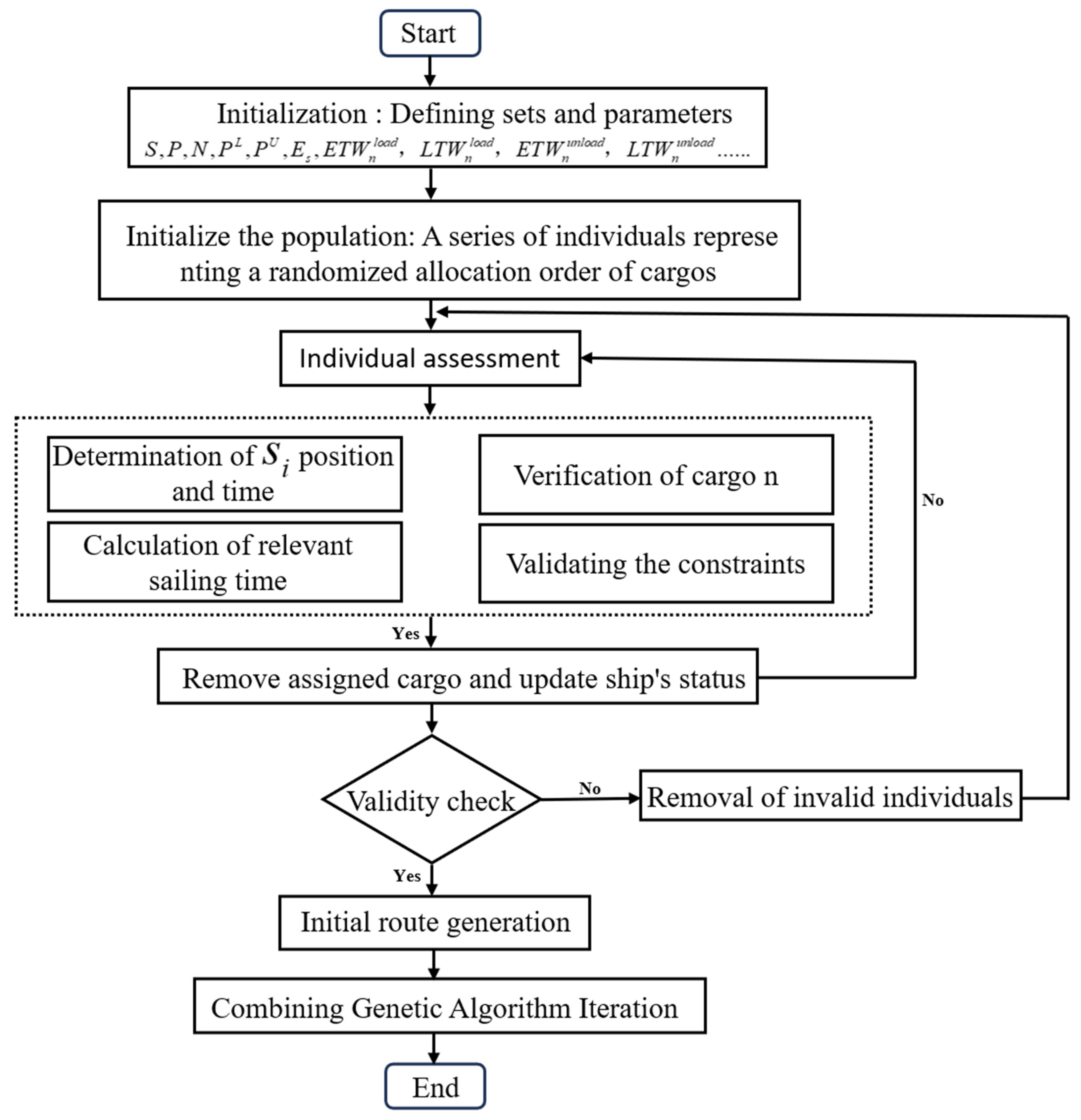
Figure 3.
(a) Pareto frontier based on sailing time and CO2 emissions for ship 1; (b) Pareto frontier based on sailing time and CO2 emissions for ship 2; (c) Pareto frontier based on sailing time and CO2 emissions for ship 3; (d) Pareto frontier based on sailing time and CO2 emissions for ship 4.
Figure 3.
(a) Pareto frontier based on sailing time and CO2 emissions for ship 1; (b) Pareto frontier based on sailing time and CO2 emissions for ship 2; (c) Pareto frontier based on sailing time and CO2 emissions for ship 3; (d) Pareto frontier based on sailing time and CO2 emissions for ship 4.


Figure 4.
Simulation of the actual route of the ship concerning ship 1.

Figure 5.
Performance of ship 1 under multi-speed sailing conditions.
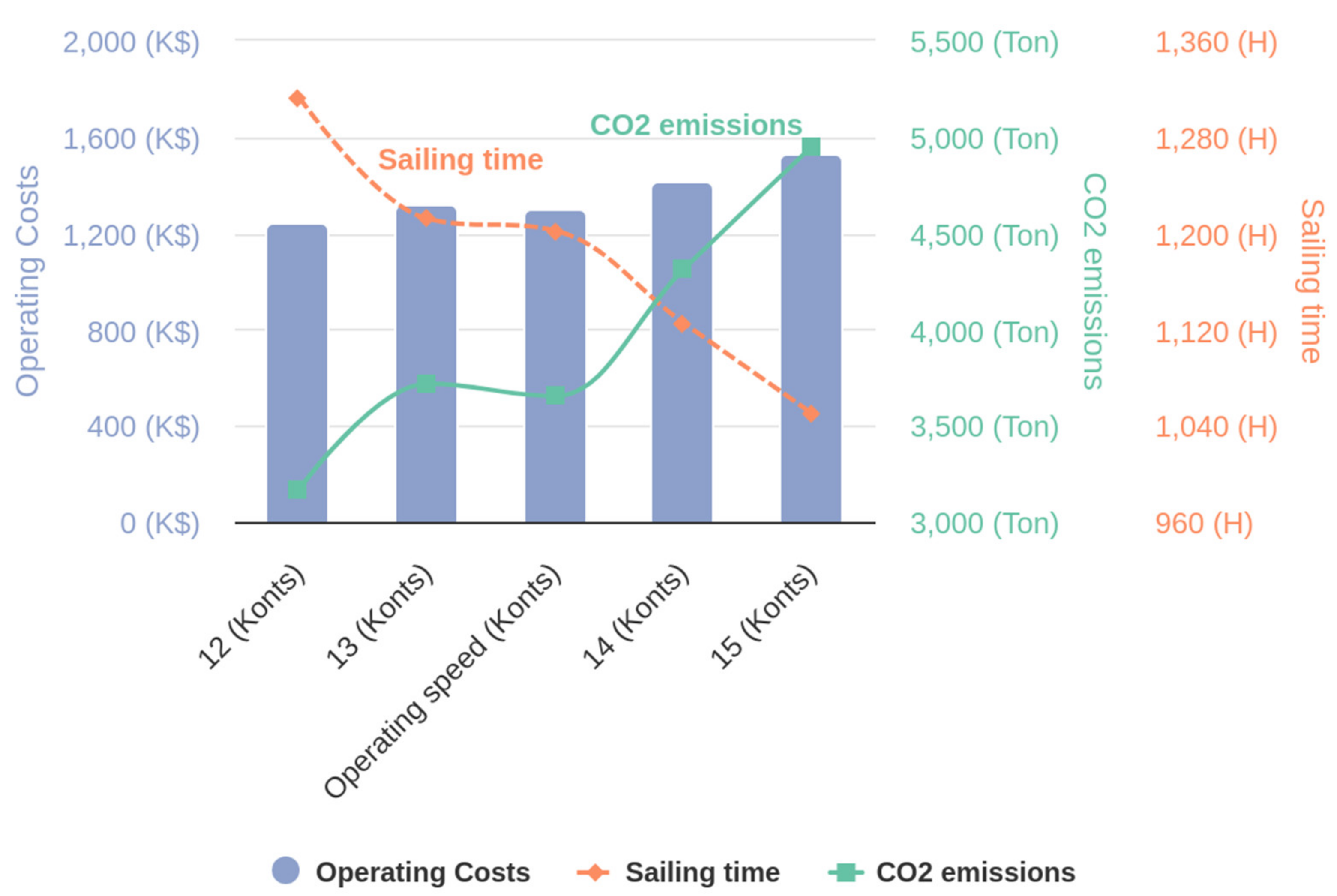
Figure 6.
Performance of ship 2 under multi-speed sailing conditions.

Figure 7.
Performance of ship 3 under multi-speed sailing conditions.

Figure 8.
Performance of ship 4 under multi-speed sailing conditions.

Figure 9.
Analysis of fleet performance indicators under multi-speed sailing conditions.

Figure 10.
Sailing time, CO2 emissions, and operating costs with different time weights.

Table 1.
Parameter and variable sets.
| Tag | Description |
|---|---|
| Set | |
| S | Set of ships, S = 1, 2, 3… |
| P | Set of ports, P = 1, 2, 3… |
| Set of loading ports | |
| Set of unloading ports | |
| N | Set of cargoes |
| L | Set of feasible voyage routes, L = 1, 2, 3… |
| Set of empty weights for ship s | |
| Parameters | |
| Fuel consumption for voyage route l of ship | |
| Emission factor, a constant | |
| A constant | |
| Cargo weight carried by ship s | |
| o(s) | Initial position of ship s |
| d(s) | Destination node in the solution or the destination port of the ship s |
| Earliest loading time for cargo n | |
| Latest loading time for cargo n | |
| Earliest unloading time for cargo n | |
| Latest unloading time for cargo n | |
| Fuel price | |
| Daily fixed cost | |
| Distance from port i to port j | |
| m | Number of ships, a constant |
| Variables | |
| Variable defining ship s sailing from i to j as 0,1 | |
| Total sailing time for the fleet | |
| Sailing time for the current voyage | |
| Ballast speed of ship s | |
| Fully loaded speed of ship s | |
| CO2 emissions for voyage route l of the ship | |
| Operating costs for ship | |
| CO2 emissions for voyage route l of the ship | |
| Total CO2 emissions for the fleet |
Table 2.
Ship data information.
| Ship ID | Initial Port | Initial Time (H) | Speed Range (Knots) | Capacity (Tons) | Empty Weight (Tons) | Daily Cost ($) | |
|---|---|---|---|---|---|---|---|
| Min | Max | ||||||
| 1 | Sydney | 288 | 11.5 | 17 | 31,760 | 13,382 | 5200 |
| 2 | Belem | 96 | 11 | 16 | 32,800 | 14,295 | 5800 |
| 3 | New Orleans | 24 | 11 | 17 | 31,770 | 11,936 | 5300 |
| 4 | Rotterdam | 168 | 10 | 16 | 34,650 | 14,273 | 6200 |
Table 3.
Cargo data information.
| Cargo ID | Cargo Weight (Tons) | Load Port | Unload Port | Load Time Start (H) | Load Time End (H) | Unload Time Start (H) | Unload Time End (H) | Charter Cost (K$) |
|---|---|---|---|---|---|---|---|---|
| 1 | 27,050 | Sydney | Ho Chi Minh | 270 | 298 | 572 | 667 | 872 |
| 2 | 24,728 | Rotterdam | Fujairah | 150 | 220 | 576 | 693 | 633 |
| 3 | 24,814 | Belem | Qingdao | 94 | 144 | 815 | 1026 | 926 |
| 4 | 29,304 | New Orleans | Le Havre | 22 | 126 | 330 | 422 | 437 |
| 5 | 30,576 | Vancouver | Dalian | 843 | 1063 | 1182 | 1485 | 517 |
| 6 | 24,975 | Vancouver | Guangzhou | 2011 | 2481 | 2392 | 2561 | 581 |
| 7 | 31,733 | Dunkerque | Port Klang | 983 | 1023 | 1528 | 1881 | 755 |
| 8 | 29,862 | Seattle | Tokyo | 1529 | 1921 | 1813 | 2270 | 409 |
| 9 | 30,616 | Sydney | Fujairah | 867 | 1031 | 1330 | 1605 | 639 |
| 10 | 28,879 | Vancouver | Ningbo | 1160 | 1447 | 1516 | 1866 | 511 |
| 11 | 27,365 | Seattle | Guangzhou | 1855 | 2298 | 2229 | 2573 | 550 |
Table 4.
Detailed analysis of the ship’s operational efficiency.
| ID | Route | Cargoes | Ballast Speed (Knots) | Full Load Speed (Knots) | Fuel Consumption (Tons) | CO2 Quantity (Tons) | Time (H) | Time Cost (K$) | Fuel Cost (K$) |
|---|---|---|---|---|---|---|---|---|---|
| 1 | 1-1-8 | 1 | - | 12.7 | 427.7 | 1154.7 | 347 | 141.82 | 256.60 |
| 1 | 8-1-9 | 9 | 14.9 | 12.4 | 925.5 | 2498.9 | 855 | 348.99 | 555.30 |
| 2 | 3-3-10 | 3 | - | 13 | 1048.8 | 2831.7 | 849 | 325.39 | 629.26 |
| 2 | 10-5-16 | 10 | 14.8 | 12.5 | 795.1 | 2146.7 | 747 | 286.33 | 477.05 |
| 2 | 16-7-13 | 11 | 14.7 | 12.3 | 840.0 | 2268.1 | 818 | 313.58 | 504.02 |
| 3 | 4-4-11 | 4 | - | 12.4 | 389.3 | 1051.0 | 377 | 135.16 | 233.56 |
| 3 | 11-5-12 | 5 | 14.9 | 12.3 | 828.4 | 2236.7 | 928 | 332.65 | 497.04 |
| 3 | 12-7-15 | 8 | 14.9 | 12.1 | 621.1 | 1676.9 | 700 | 250.98 | 372.65 |
| 4 | 2-2-9 | 2 | - | 12.3 | 604.9 | 1633.2 | 505 | 237.84 | 362.94 |
| 4 | 9-6-14 | 7 | 14.7 | 12.3 | 1236.6 | 3338.9 | 1075 | 506.12 | 741.99 |
| 4 | 14-5-13 | 6 | 14.8 | 12.6 | 1064.6 | 2874.5 | 946 | 445.20 | 638.78 |
Sydney: 1; Rotterdam: 2; Belem: 3; New Orleans: 4; Vancouver: 5; Dunkerque: 6; Seattle: 7; Ho Chi Minh: 8; Fujairah: 9; Qingdao: 10; Le Havre: 11; Dalian: 12; Guangzhou: 13; Port Klang: 14; Tokyo: 15; Ningbo: 16.
Table 5.
Summary of ship operating costs.
| ID | Fuel Consumption (Tons) | CO2 Quantity (Tons) | Time (H) | Time Cost (K$) | Fuel Cost (K$) | Total Cost (K$) |
|---|---|---|---|---|---|---|
| 1 | 1353.2 | 3653.6 | 1202 | 490.8 | 811.9 | 1302.7 |
| 2 | 2683.9 | 7246.5 | 2414 | 925.3 | 1610.3 | 2535.6 |
| 3 | 1838.7 | 4964.6 | 2006 | 718.8 | 1103.2 | 1822.0 |
| 4 | 2906.2 | 7846.7 | 2526 | 1189.2 | 1743.7 | 2932.9 |
| Total | 8782.0 | 23,711.4 | 8147 | 3324.1 | 5269.2 | 8593.2 |
Table 6.
CO2 emissions, sailing time, and operating costs at speeds 12 & 13 knots data table.
| Speed 12 Knots | Speed 13 Knots | Operating Speed | |||||||
|---|---|---|---|---|---|---|---|---|---|
| ID | CO2 (Tons) | Time (H) | Cost (K$) | CO2 (Tons) | Time (H) | Cost (K$) | CO2 (Tons) | Time (H) | Cost (K$) |
| 1 | 3167.6 | 1313 | 1240.1 | 3717.5 | 1212 | 1321.0 | 3653.6 | 1202 | 1302.7 |
| 2 | 6088.8 | 2675 | 2378.6 | 7145.9 | 2470 | 2534.6 | 7246.5 | 2414 | 2535.6 |
| 3 | 4194.4 | 2244 | 1736.1 | 4922.5 | 2071 | 1836.1 | 4964.6 | 2006 | 1822.0 |
| 4 | 6719.7 | 2789 | 2806.2 | 7886.3 | 2574 | 2964.5 | 7846.7 | 2526 | 2932.9 |
Table 7.
CO2 emissions, sailing time, and operating costs at speeds 14 & 15 knots data table.
| Speed 14 Knots | Speed 15 Knots | Operating Speed | |||||||
|---|---|---|---|---|---|---|---|---|---|
| ID | CO2 (Tons) | Time (H) | Cost (K$) | CO2 (Tons) | Time (H) | Cost (K$) | CO2 (Tons) | Time (H) | Cost (K$) |
| 1 | 4311.4 | 1126 | 1417.7 | 4949.3 | 1050 | 1528.8 | 3653.6 | 1202 | 1302.7 |
| 2 | 8287.6 | 2293 | 2720.7 | 9513.8 | 2140 | 2934.6 | 7246.5 | 2414 | 2535.6 |
| 3 | 5709.0 | 1923 | 1957.8 | 6553.7 | 1795 | 2099.6 | 4964.6 | 2006 | 1822.0 |
| 4 | 9146.3 | 2390 | 3157.9 | 10,499.6 | 2231 | 3383.6 | 7846.7 | 2526 | 2932.9 |
Table 8.
Decision options table.
| Keys | Option | |||
|---|---|---|---|---|
| Decision 1 | Decision 2 | Decision 3 | Decision 4 | |
| CO2 (Tons) | 16,948.8 | 17,480.1 | 19,131.0 | 23,711.4 |
| Time (H) | 9841 | 9624 | 9071 | 8147 |
| Cost (K$) | 7779.5 | 7804.2 | 7951.9 | 8593.2 |
Disclaimer/Publisher’s Note: The statements, opinions and data contained in all publications are solely those of the individual author(s) and contributor(s) and not of MDPI and/or the editor(s). MDPI and/or the editor(s) disclaim responsibility for any injury to people or property resulting from any ideas, methods, instructions or products referred to in the content. |
© 2024 by the authors. Licensee MDPI, Basel, Switzerland. This article is an open access article distributed under the terms and conditions of the Creative Commons Attribution (CC BY) license (https://creativecommons.org/licenses/by/4.0/).
Share and Cite
MDPI and ACS Style
Huang, X.; Liu, Y.; Sha, M.; Han, B.; Han, D.; Liu, H. ETE-SRSP: An Enhanced Optimization of Tramp Ship Routing and Scheduling. J. Mar. Sci. Eng. 2024, 12, 817. https://doi.org/10.3390/jmse12050817
AMA Style
Huang X, Liu Y, Sha M, Han B, Han D, Liu H. ETE-SRSP: An Enhanced Optimization of Tramp Ship Routing and Scheduling. Journal of Marine Science and Engineering. 2024; 12(5):817. https://doi.org/10.3390/jmse12050817
Chicago/Turabian StyleHuang, Xiaohu, Yuhan Liu, Mei Sha, Bing Han, Dezhi Han, and Han Liu. 2024. "ETE-SRSP: An Enhanced Optimization of Tramp Ship Routing and Scheduling" Journal of Marine Science and Engineering 12, no. 5: 817. https://doi.org/10.3390/jmse12050817
Note that from the first issue of 2016, this journal uses article numbers instead of page numbers. See further details here.