
The Machine Learning Attribution of Quasi-Decadal Precipitation and Temperature Extremes in Southeastern Australia during the 1971–2022 Period


1
School of Mathematical and Physical Sciences, University of Technology Sydney, 15 Broadway, Ultimo, NSW 2007, Australia
2
The Climate Risk Group, Newcastle, NSW 2300, Australia
*
Author to whom correspondence should be addressed.
Climate 2024, 12(5), 75; https://doi.org/10.3390/cli12050075
Submission received: 1 April 2024
/
Revised: 11 May 2024
/
Accepted: 13 May 2024
/
Published: 17 May 2024
(This article belongs to the Special Issue Addressing Climate Change with Artificial Intelligence Methods)
Abstract
:Much of eastern and southeastern Australia (SEAUS) suffered from historic flooding, heat waves, and drought during the quasi-decadal 2010–2022 period, similar to that experienced globally. During the double La Niña of the 2010–2012 period, SEAUS experienced record rainfall totals. Then, severe drought, heat waves, and associated bushfires from 2013 to 2019 affected most of SEAUS, briefly punctuated by record rainfall over parts of inland SEAUS in the late winter/spring of 2016, which was linked to a strong negative Indian Ocean Dipole. Finally, from 2020 to 2022 a rare triple La Niña generated widespread extreme rainfall and flooding in SEAUS, resulting in massive property and environmental damage. To identify the key drivers of the 2010–2022 period’s precipitation and temperature extremes due to accelerated global warming (GW), since the early 1990s, machine learning attribution has been applied to data at eight sites that are representative of SEAUS. Machine learning attribution detection was applied to the 52-year period of 1971–2022 and to the successive 26-year sub-periods of 1971–1996 and 1997–2022. The attributes for the 1997–2022 period, which includes the quasi-decadal period of 2010–2022, revealed key contributors to the extremes of the 2010–2022 period. Finally, some drivers of extreme precipitation and temperature events are linked to significant changes in both global and local tropospheric circulation.
1. Introduction
Global warming (GW) has accelerated in recent decades, with precipitation and temperature extremes becoming more common [1,2,3]. It is known from previous studies, e.g., [4,5], that water availability in southeastern Australia (SEAUS, Figure 1) has been diminishing in both quantity and quality owing to a combination of prolonged dry periods and a rapidly increasing population. Consequently, to assist in increasing water sustainability and preparing for increased heatwave frequency, there is a need to examine the complex relationships between changes in the patterns of precipitation and higher temperatures resulting from the impacts of ocean and atmospheric climate drivers affecting SEAUS. GW increases the frequency and intensity of extreme precipitation and heatwaves and associated floods and droughts by amplifying the effects of the various SEAUS climate drivers [4,5]. Accordingly, despite the mean annual rainfall remaining at the same level, the SEAUS water supply has become less reliable because of dramatically increased rainfall variability. Notwithstanding the recent wet years of the 2020–2022 period, parts of SEAUS have exhibited a rapid return to heat waves and drought conditions in 2023 and 2024. Prior to the accelerated GW period dating from the early 1990s, seasonal and annual precipitation extremes were typically measured over much longer time periods (e.g., 30 years or more) [6]. Given that the climate can no longer be regarded as stationary (as mentioned, e.g., in [7,8]), in this study, we focused on the most recent 13-year period, 2010–2022, in which numerous precipitation and temperature extremes occurred in SEAUS. This period in SEAUS also encapsulates the global trend towards increasingly intense rainfall and temperature events [9,10]. There is a need to assess the implications for extreme precipitation and temperature events in SEAUS on shorter, quasi-decadal time periods with a focus on the exemplar period of 2010–2022. The requirement for important environmental policy decisions based on these briefer time periods has become increasingly essential.
During the 2010–2022 period, much of SEAUS experienced both extreme rainfall events and severe hot, dry periods, leading to fluctuations between unprecedented floods and droughts. In terms of climate drivers, the double La Niña event of the 2010–2012 period immediately followed the Millennial Drought event. Owing primarily to the La Niña event and subsequent rain-bearing low-pressure systems, the summer of the 2010/2011 period was the wettest on record in Australia [11]. In addition, the abnormally strong La Niña event of the 2010/2011 period was immediately followed by another La Niña event in the 2011/2012 period, making the two-year period of 2010–2012 the most significant two-year La Niña period since at least the 1973–1976 period, and possibly since the 1917–1918 period. Another notable feature of the 2010–2012 La Niña was the number of rainfall events that affected many regions across SEAUS. Summer (DJF) is typically the driest time of year in the southern part of SEAUS, but instead, it experienced extreme rainfall events and floods. In parts of northern SEAUS, catastrophic flooding occurred in the summer of 2011.
In contrast, drought returned in the 2013–2019 period, and many parts of inland SEAUS suffered from water shortages, culminating in the need for drinking water to be transported into towns. The 2017–2019 period reached decile 1 with the lowest rainfall records established in parts of SEAUS (Figure 2a). During this period, many inland dams that use water for irrigating crops and supplying drinking water reached critically low levels in many communities. However, within this 2013–2019 period, in 2016, there was a brief but contrasting period of flooding in inland SEAUS when a strongly negative phase of the Indian Ocean Dipole (IOD) [12] resulted in extreme late winter/spring rainfall. The negative IOD phase produced anomalously high sea surface temperatures (SSTs) in the east Indian Ocean that enhanced atmospheric moisture and generated rain-bearing systems across southern Australia. Combined with atmospheric moisture from the Pacific Ocean across the Australian east coast, extreme late winter/spring rainfall and flooding affected many river systems over inland SEAUS.
Another negative IOD phase in 2022 was a key factor in producing extreme rainfall and the worst flooding on record in northern parts of Victoria and southwest New South Wales during the spring months of September/October. In addition, the third year of a triple La Niña (2020–2022) affected SEAUS (Figure 2b) in contrast to the previous three drought years of 2017–2019 (Figure 2b). Figure 2b shows the highest rainfall recorded in the same area of SEAUS as the drought in Figure 2a. Many SEAUS rainfall records were broken in early 2022, with catastrophic flooding occurring in the city of Lismore, located just 50 km inland from Yamba on the coast (Figure 1). Sydney (Figure 1), which is Australia’s most populous city, also suffered catastrophic river flooding in 2022 while setting a new annual rainfall record since observations began in 1859.
Along with rising GW in 2022, SEAUS experienced both a La Niña event and a negative IOD. Compounding climate drivers can magnify their impacts, leading to extremes in rainfall and run-off. For example, in a subset of inland SEAUS between 25° and 40° S, a key finding of the impacts on water supply is the presence of both local and global sea surface temperatures with the attributes of ENSO, the southern annular mode (SAM) [13], and the IOD, either individually or in combination [5]. To detect oceanic and atmospheric climate drivers or combinations of climate drivers that are responsible for the precipitation extremes affecting SEAUS, including the 2010–2022 period, we use machine learning (ML) attribution techniques. ML is applied to the high-quality precipitation records of eight Australian Bureau of Meteorology (BoM) observation stations using data from the BoM climate change network. The selected stations are representative of SEAUS. The remainder of this study describes the study area, provides a data analysis of the time series of rainfall and temperature in SEAUS, and describes the ML techniques applied to the data. These are followed by the results, the statistical significance of those groupings, and the ranking of the most important climate driver attributes, and it ends with the Section 4.
2. Materials and Methods
2.1. Study Area
The eight stations representative of subtropical SEAUS (Figure 1) were chosen for this study because of their complete BoM records of precipitation and temperature from 1970 to mid-2023 [14]. Geographically, the four northern-most sites (Barcaldine, Yamba, White Cliffs, and Clarence Town), hereafter referred to as N, were grouped for analysis because they are located close to the tropics, whereas the four southern sites (Wakool, Orbost, Wilsons Promontory, and Sorell), hereafter referred to as S, were grouped because they almost reach the mid-latitudes. As such, the N and S stations have different climate regimes. An east and west grouping of the stations was deemed unnecessary because coastal precipitation in the study area is known to have declined in every decade since 1970 [4].
2.2. Data
Accelerated GW since the early 1990s has been accompanied by changes in precipitation and maximum temperatures across SEAUS. To assess the impacts of various climate drivers on these trends, ML techniques were applied to selected climate drivers as described below. They include Atlantic Multi-decadal Oscillation (AMO), the Dipole Mode Index or Indian Ocean Dipole (IOD), Global Sea Surface Temperature Anomalies (GlobalSSTA), Global Temperature Anomalies (GlobalT), Niño3.4, the Tripole Index for the Interdecadal Pacific Oscillation (TPI), the Southern Annular Mode (SAM), and the Southern Oscillation Index (SOI). These data are all readily accessible from the NOAA Physical Sciences Laboratory on the following website: https://psl.noaa.gov/gcos_wgsp/Timeseries/ (accessed on 1 April 2024). The monthly Pacific Meridional Mode (PMM), which is often referred to as the North Pacific Meridional Mode (NPMM), is available at https://psl.noaa.gov/data/timeseries/monthly/PMM/ (accessed on 1 April 2024). Additionally, Tasman Sea Surface Temperature anomalies (TSSST) are obtained from the BoM website [15]. Two-way interactions between climate drivers, which are obtained by multiplying any two of these climate drivers together (e.g., AMO*IOD), were also considered potential attributes. These techniques were applied to the data from 1970 to 2022.
2.3. Methods
Machine learning (ML) techniques, which are described in Section 2.3, will be applied to the eight observation stations shown in Figure 1. The time series of precipitation and the mean maximum temperature (TMax) were first plotted, along with their percentiles. The data were assessed both annually and over the multiple monthly groupings of the April–May, December–March, and July–November periods. These monthly groupings were selected because, for a large subset of SEAUS, in the Murray–Darling Basin (MDB), it has been shown that rainfall in the April-May period has decreased significantly since the 1990s [5,16]. The December-March summer period is important for parts of SEAUS owing to the strong relationship with the phase of ENSO, and hence, rainfall variability [17] in addition to the phase of the SAM. Similarly, rainfall in the July–November period is influenced by the phase of the IOD in addition to ENSO.
Previous studies of areas within SEAUS permutation testing of precipitation and temperature have shown statistical significance before and after the mid-1990s [5,18]. Therefore, the data are non-stationarity, and a change-point analysis was not applicable. The data were then grouped into two consecutive 26-year splits, 1971–1996 and 1997–2022, and since our main aim was to investigate the precipitation and maximum temperature extremes of the quasi-decadal period of 2010–2022, four equal 13-year (quasi-decadal) splits were made beginning in 1971 and ending in 2022. Two-sided permutation testing was applied to build sampling distributions using 5000 resamples without replacement. This allowed for the evaluation of statistically significant differences in values, such as the mean or variance, between any two time periods.
To attribute the above climate drivers to the different precipitation periods considered, ML was applied with sliding window cross-validation [19], where the initial training window contained 20 years of data, and the testing window was fixed to contain the following 20 years of data. This method resulted in 14 models being developed for each statistical modelling technique. The considered models were linear regression (LR), support vector regression (SVR) with both radial basis function (RBF) and polynomial (Poly) kernels, and random forest (RF). To select the attributes, both forward and backward selection techniques were applied [20]. We note that the overfitting of data was avoided by using sliding window cross-validation because it ensures that training data does not overlap with testing data.
3. Results
Differences in the means and variances for precipitation and TMax for SEAUS and the two northern and southern subset regions of SEAUS, referred to here as N and S, between the 1971–1996 and 1997–2022 periods are shown in Table 1. The time series of precipitation and TMax for the three areas are shown in Figure 3, Figure 4 and Figure 5.
3.1. Precipitation and TMax Time Series for SEAUS
The annual total precipitation time series for SEAUS reveals that there was no trend since 1970, and the mean p-value (0.38; Table 1) between the 1971–1996 and 1997–2022 periods is not significant. However, there is clearly greater variance from 2010 to 2022 because of the many, almost equal, number of years either above or below the 50th percentile (Figure 3a). By season, the decreased precipitation variance in the April-May period between the 1971–1996 and 1997–2022 periods is significant (p-value = 0.055; Table 1). There is a clear increasing trend in the mean TMax from the 1990s, with all p-values being statistically significant or highly significant (Table 1). However, the variance is not significantly different between the two 26-year intervals. The influence of ENSO is clearly seen in December to March by the increased precipitation during both the multi-year La Niña events of the 1973–1976 and 2020–2022 periods and less so during the 2010–2012 La Niña period. The mean TMax value for the April–May period shows an increasing trend (mean p-value = 0.07; Table 1) accompanied by increased variability starting from 2010. The precipitation from July to November indicates no trend, although the two years of 2010 and 2022 above the 95th percentile are investigated later through ML to determine whether a combined contribution from IOD and La Niña are important. Again, the mean TMax value shows an increasing trend in the period from July to November except during all three La Niña periods, 1973–1976, 2010–2012, and 2020–2022, as expected. The mean TMax p-value of zero (Table 1) reveals a highly significant decrease in the mean of the 26-year 1971–1996 period compared with the latest 26-year period of 1997–2022. For both the December to March period and July to November period, there is no statistical significance in precipitation. There is a high statistical significance in the mean TMax value (p-value = 0.0006 rounded to 0; Table 1) but no statistical significance in variance.
3.2. Total Precipitation and TMax Time Series of N
As for SEAUS, there is no trend in annual precipitation in N. Apart from the extreme rainfall in the La Niña years, there is a sharp contrast between the extremely low rainfall in 2019 at the end of the 3-year drought to the extreme rainfall in 2022, which was influenced by a strong La Niña event (Figure 4a). This is reflected in the large TMax variability from 2010 caused by the 2017–2019 drought period between the 2010 and 2022 La Niña years. However, the difference in the variance between the 26-year periods of 1971–1996 and 1997–2022 is not significant (Table 1). Also, there are no significant differences for the monthly groupings of April–May, December to March, and July–November. For the April–May period, the driest years are becoming drier, with 9 years being below the 25th percentile after the 1990s compared to 2 years prior to the 1990s. There is a clear increasing trend in the mean TMax value, especially from 2011. The difference between the 1971–1996 and 1997–2022 periods for the April–May mean TMax value is significant (p-value = 0.05; Table 1). December to March highlights the large total precipitation in the La Niña periods of 1973–1976 and 2020–2021 and an increasing trend in the TMax value, especially after 2010, with a highly significant p-value between the 1971–1996 and 1997–2022 periods (p-value = 0.007; Table 1). While precipitation from July to November shows no trend, the 4 years at the 95th percentile or above were during La Niña phases, in addition to the IOD in 2010 and 2022 being strongly negative during the July to November period, which acts as an enhancement to rainfall in SEAUS. The increasing trend in the TMax value for the July–November period is evident from the 1990s (Figure 4f), and the mean TMax value is highly significant (p-value = 0.001 rounded to zero; Table 1).
3.3. Total Precipitation and TMax Time Series of S
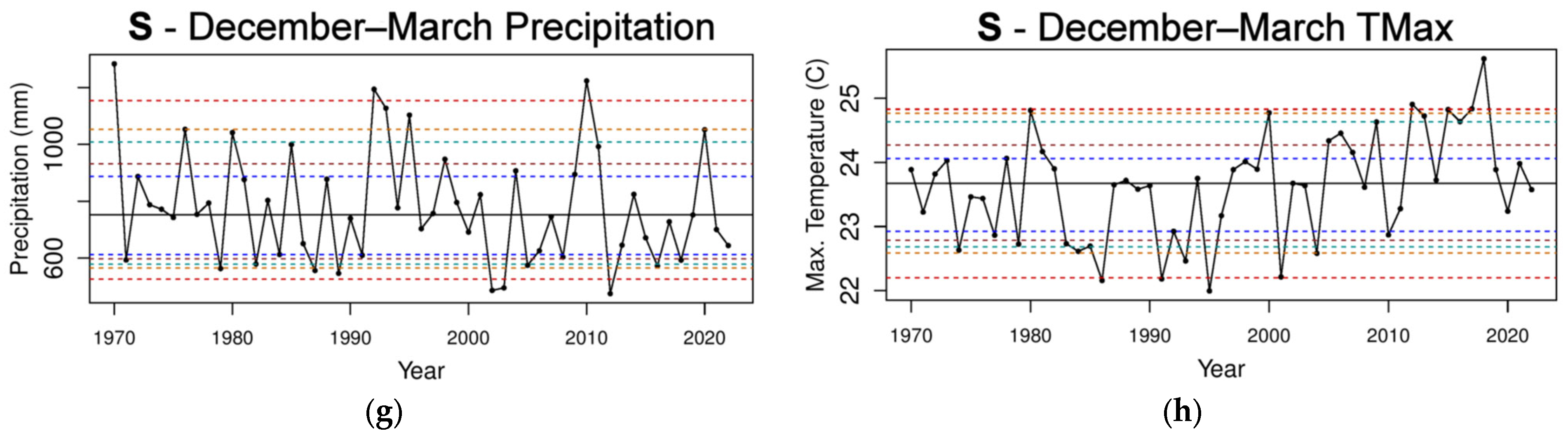
Annual precipitation in S shows a slightly decreasing trend in the median (Figure 5a), and the mean (p-value = 0.06; Table 1) has decreased significantly from the 1971–1996 period to the 1997–2022 period. An increase in the TMax value is clearly visible from 1997 (Figure 5b), and the mean is highly significant (p-value = 0; Table 1). While the mean precipitation change in the April–May period is not statistically significant, there is a marked decrease in the number of high rainfall years with no values above the 90th percentile except for 2022 (Figure 5c). Consequently, there is a significant decrease in variance in the April–May period from the 1971–1996 period to the 1997–2022 period (p-value = 0.086; Table 1). There is only a slight upward trend in the mean TMax value mainly because of the three values above the 95th percentile after 1997 (Figure 5c). These three values contribute to the upward (though non-significant) trend in the mean TMax value (p-value = 0.19; Table 1). In the December–March period, there is no statistically significant change in precipitation. However, there is a decrease in the lowest percentiles, with three yearly values below the 5th percentile after 1997 compared to zero before 1997 (Figure 5g). The upward trend in the TMax value from the late 1990s is clearly visible (Figure 5h) and is highly significant for the mean TMax value (p-value = 0.001, rounded to zero; Table 1). The pattern for precipitation in the July–November period continues with nine values at or below the 20th percentile from the mid-1990s compared to one value prior to the mid-1990s (Figure 5e), and there is a significant decrease in mean precipitation (p-value = 0.075; Table 1), which indicates that the July–November period is the main contributor to the significant decrease in the annual mean precipitation. The mean TMax value for the July–November period is highly significant (p-value = 0; Table 1).
3.4. Total Precipitation and TMax p-Values for Six Quasi-Decadal Intervals
The total precipitation means were assessed for significance between the six 13-year (quasi-decadal) intervals shown in Table 2. Focusing on the two most recent intervals of 1997–2009 and 2010–2022, they show no significant difference in means except for the April–May period for the S area (p-value = 0.075; Table 2) owing largely to the two outlier values at the 90th and 95th percentiles in 2020 and 2022 (Figure 5c), respectively. There is no significant change in variance. In the earlier quasi-decadal intervals, there are significant changes in some of the means and variances for mean total precipitation because those quasi-decadal splits capture large groups of months when extremely low rainfall is followed by extremely high rainfall (e.g., 1997–2009 and 2010–2022 for July–November), or extremely high rainfall is followed by extremely low rainfall (e.g., 1971–1983 and 1997–2009 for April–May in SEAUS and S, or 1984–1996 and 1997–2009 for annual precipitation and July–November in S). In N, there are no quasi-decadal intervals exhibiting statistical significance in the mean nor the variance. In S, the annual variance is statistically significant (p-value = 0.033; Table 2) from high precipitation to low precipitation in the quasi-decadal split of the 1971–1983 and 1997–2009 periods, as is the April–May variance for the 1971–1983 period compared with the 1984–1996 period (p-value = 0.042). This is consistent in S with statistical significance of variance for precipitation in the April–May period in the 26-year split of 1971–1996 and 1997–2022. There is statistical significance for the July–November decrease in mean between the 1984–1996 and 1997–2009 periods. For the December–March period, there is no statistical significance for the mean nor variance in the S area.
For the TMax means, the 13-year intervals show significance in the two splits prior to 1997 with the two splits from 1997 (Table 3). Either significance or high significance is present in the annual, April–May, July–November, and December–March values for SEAUS, N, and S. In comparison, only the April–May TMax mean in S is not significant for the 26-year split between the 1971–1996 and 1997–2022 periods, even though there are three values above the 95th percentile after 1997 compared to none before 1997 (Figure 5d). In general, the statistical significance in the mean TMax value, as shown between the decadal intervals and the 26-year interval, highlights the increase in global warming from 1971. The TMax variance highlights the statistical significance for annual variance in SEAUS and N between the 1997–2009 and 2010–2022 periods owing to the larger spread within the 2010–2022 period.
3.5. Attribute Selection
Table 4 summarises the climate drivers of greatest influence on both the range of time scales from annual to monthly groupings and for each region of SEAUS. The five most significant attributes for each area and for each monthly group, consisting of greater than or equal to 50% mean folds across the eight ML methods, were obtained by using a sliding training window with a size of 20 and a fixed testing window with a size of 20. The selection process for the most prominent attributes is shown in the Supplementary Materials for just one of the twelve possible combinations of time periods and regions, namely for the annual time period and the entire SEAUS. It shows that all 12 combinations would be prohibitive in size and unnecessary as the same process is used in each time period and region. For total precipitation in SEAUS, the oceanic climate drivers dominate the annual time period. The first is AMO*PMM. AMO is a remote Atlantic climate driver that is linked with the local Pacific climate drivers of PMM and IOD, with Niño3.4 being influential by itself. For the April–May and July–November periods, the ocean climate drivers again dominate either singularly or in combination with other drivers. As an atmospheric climate driver, the SOI is also important because it favours a moist, easterly wind regime in the spring/summer in its positive phase. For the July–November period, the IOD features strongly, which is consistent with its known late winter/spring influence on rainfall across SEAUS. For both the December–March and April–May periods, it is interesting that the IOD is an important influence. This will be discussed in the next section. For area N, the ocean climate drivers are again prominent. However, in both the July–November and annual periods, the atmospheric climate drivers SAM and SOI have the most influence. For area S, the IOD becomes the dominant annual influence, which is consistent with the July–November period. However, for the December–March period, the atmospheric climate driver, the SOI, in combination with local Tasman Sea temperatures is the most dominant influence.
4. Discussion
During the 2010–2012 period, SEAUS experienced precipitation and maximum temperature extremes, with record-breaking rainfall in the La Niña event from 2010 to 2012, which was immediately followed by catastrophic drought during the 4-year period from 2016 to 2019 [21]. This study found that the mean annual precipitation of the groupings, namely the annual, April–May, July–November, or December–March periods, for all of SEAUS and the individual N region has not changed significantly between the 1971–1996 and 1997–2022 periods (Table 1). In contrast, the mean annual precipitation significantly decreased in area S (p-value = 0.06; Table 1) largely due to a significant decrease in the July–November period’s mean precipitation (p-value = 0.075; Table 1). The variability of total precipitation in the April–May period decreased significantly in SEAUS (p-value = 0.055; Table 1) due to a significant decrease in the variability in S (p-value = 0.086), with no values above the 80th percentile after 1997 (Figure 5c). Another important feature is the recent increase in the variability of precipitation in area N for December to March (Figure 4g) and July to November (Figure 4e) starting from about 2010 owing to the two extremely wet periods of 2010–2012 and 2020–2022, with the driest, consecutive 4-year period on record between them from 2016 to 2019. However, the variance in p-values between the 1971–1996 and 1997–2022 periods is not significant because there is almost an equal number of wet and dry years in both intervals. The significant increase in the mean TMax value between the 1971–1996 and 1997–2022 periods for all areas and monthly groupings, except for the April–May period in S, confirms the impact of the increase in GW.
Turning to the 13-year (quasi-decadal) intervals, the two most recent quasi-decadal intervals in the 1997–2009 and 2010–2022 periods do not show a significant change in the mean total precipitation except for the April–May period in S (p-value 0.075; Table 2), which is a significant increase largely due to the two outlying values at the 90th and 95th percentiles in 2020 and 2022, respectively. For SEAUS, it is notable that there is a significant increase in variance between the 1986–1996 and 2010–2022 periods for both the annual and December–March time periods and the annual period for S. The remainder of significant changes in either the mean or variance are decreases in significance for SEAUS and S for the two earliest decadal intervals in the 1997–2009 period. Regarding the TMax value, the statistical significance in the mean TMax value, as shown between most quasi-decadal intervals and the 26-year interval, generally confirms the increase in global warming starting from 1971. The variance in the TMax value highlights the statistical significance for annual variance in SEAUS and N between the 1997–2009 and 2010–2022 periods owing to the larger spread within the 2010–2022 period. In summary, the precipitation time series and p-values suggest that SEAUS continues to warm and hence increases in evapotranspiration despite there being more decreasing precipitation in S than in N.
An important finding revealed by the SEAUS precipitation attributes is the teleconnections between the remote Atlantic Ocean climate driver AMO and close relationships with local ocean climate drivers, such as Tasman Sea SSTs, Niño3.4 and the PMM from the Pacific Ocean, and the IOD from the Indian Ocean (see Table 4). In the presence of background GW, these attributes either amplify or diminish the impacts of extreme precipitation during the 2010–2022 period either singularly or in combination with other ocean climate drivers and atmospheric climate drivers such as SAM or SOI. Another noteworthy result is the top-ranking attribute of the combined ocean–atmospheric climate driver, IOD*SAM, for both SEAUS and N in the December–March period. The main influence that the IOD is known to have on precipitation in SEAUS is during the July–November period. For N, it is not surprising that the combination of the AMO*SAM and SAM*TSSSTA climate drivers (Table 4) strongly influences rainfall in the two multi-year La Nina phases during the 2010–2022 period because moist easterly component winds associated with SAM imply teleconnections linked to the AMO and TSSSTA. However, the dominant IOD*SAM attribute is more puzzling for the summer period from December to March and may be related to the longitudinal position of the strongest gradient in Indian Ocean SSTs. A very recent study found that for the 1997–2022 period, which includes the two quasi-decadal periods of 1997–2009 and 2010–2022 in this study, SAM is not a dominant attribute for precipitation within a subset area of N owing to changes in the tropospheric circulation within the Southern Hemisphere [21]. It is worth further investigating the relationship between the IOD and SAM for precipitation in the December–March period.
The key attributes of annual precipitation in S are similar to those found in other ML attribution studies for Canberra, Sydney, and the MDB, including ENSO, the IOD, SAM, and both local and global SSTs [5,22,23]. Like the autumn precipitation attributes for the Sydney Catchment Area, the AMO was found to heavily influence precipitation in the April–May period in combination with other drivers [22]. There were numerous attributes associated with global warming in SEAUS for precipitation over all monthly groupings except for the July–November period, while these attributes have appeared across all monthly splits in area S. Of note is the selection of GW attributes in the April–May period, where decreased variability has been observed in SEAUS and S. In addition, there has been a statistically significant reduction in April–May precipitation from the 1997–2009 period to the 2010–2022 period in S. This selection of attributes associated with GW is consistent with other studies in the region where warming attributes have been selected for modelling time series with observed changes in precipitation [5,19]. Meanwhile, there has been little association with GW attributes in the N region, where only one such attribute has been associated with precipitation in the December–March period, which aligns with the minimal statistically significant changes in precipitation characteristics for this region.
It is well documented that a mean 1 °C increase in the atmospheric temperature can potentially increase precipitation by 7%, e.g., [24]. The Clausius−Clapeyron equation suggests that the atmosphere can hold 7% more moisture for each 1 °C of heating. Rainfall extremes scale by approximately the same amount. This is part of the earth’s hydrological cycle and plays an important role in the natural greenhouse effect. It also accelerates warming because water vapor is a powerful greenhouse gas. However, for the catastrophic floods at both Grantham (southeast QLD; Figure 1) in January 2011 and Lismore (northeast NSW; Figure 1) in February 2022, the already saturated catchments played a key role. This can be explained by the large-scale climate drivers, La Niña and IOD, affecting eastern Australia through the spring and summer of the 2010–2011 period. In both cases, the local-scale meteorological factors such as coastal topography and low-pressure troughs had the heaviest rainfall, which led to catastrophic flooding.
Of importance is the fact that in the summer in the Southern Hemisphere (SH), when these floods occurred, there was only one jet stream, which was climatologically well south of the Australian continent. Therefore, slow movement or stationary waviness in the jet stream, referred to as arctic amplification for the Northern Hemispheric atmospheric circulation [25], can be ruled out. Arctic amplification occurred in the Northern Hemisphere (NH) in relation to the extreme 2019 German floods, the catastrophic Pakistan floods in 2013, the Russian heatwave of 2013, and the European heatwaves of 2003 and 2023. The key factors for both the Grantham and Lismore floods in southeastern Australia were the antecedent catchment conditions combined with the persistent large-scale atmospheric conditions conducive to the onshore flow of deep, atmospheric moisture when smaller spatial and temporal-scale low-pressure troughs had the heaviest rain. In other words, during moderate to strong La Niña summer phases, trending toward a positive SAM in the 2020–2022 period, which is characterised by deep, moist onshore winds onto the east coast with persist rain on saturated catchments, the possibility increases for catastrophic floods in areas when local-scale features such as topography interact with the small-scale meteorological processes associated with small, weak, short-lived low-pressure systems. Moreover, during strong La Niña phases, the polar jet is further equatorward than normal, and [26,27] showed that upper tropospheric instability in the form of relative vorticity circulations are prone to break off and head more equatorward, which reveals for the first time, to our knowledge, that the dice are loaded even further for extreme flood-producing rainfall over SEAUS when combined with the smaller spatial and temporal-scale features mentioned above. In the Sydney metropolitan area, even without strong topographic forcing, these surface to upper tropospheric meteorological features are the most common cause for severe flash flood-producing rainfall that can occur at any time of year [28]. A key factor of flash flood-producing rainfall is the slow, almost stationary nature of the upper vorticity circulation without a jet stream by the time it develops over southeast Australia. Another form of a low-pressure system that develops when the branch of the subtropical jet in the upper troposphere affects SEAUS, mainly during the cool season (April–September), is the east coast low (ECL). These systems have been responsible for many coastal, rain-producing floods in SEAUS [29,30,31]. However, their characteristics have changed in recent decades such that they now mostly develop further south along the coast and further east off the coast [32], and there are less cut-off rain-producing low-pressure systems over inland SEAUS [33].
We focused on the most recent 2010–2022 period due to the fluctuations between extreme rainfall and drought years that occurred in SEAUS during that period. The fluctuations occurred mainly because of the much larger rainfall in La Niña years than non-La Niña years. However, the 1997–2009 quasi-decadal split was also a period of extremely low rainfall and drought in SEAUS. Our analysis of the four quasi-decadal splits highlights how rainfall extremes have increased since the first two quasi-decadal splits owing to the background influence of GW. Finally, we note that the MDB with its complex river system, which occupies most of inland SEAUS, is already heading for reduced potable and agricultural water supply through the spring and summer in 2023 and 2024 owing largely to the current El Niño phase of ENSO, thereby continuing the long-term impacts of GW on decreasing water availability despite record rainfall and floods during the recent 2020–2022 La Niña period. The MDB has been drying since the 1990s because the catchment rainfall in all dams, in both the northern and southern MDB, has decreased significantly in the April-May period and continues to dry throughout the winter, even with an average or slightly below average winter rainfall. Consequently, the spring and summer soil and vegetation moisture levels will be very low. Sufficient soil moisture must be present in the spring to maintain moisture levels leading into summer. The cycle continues and progressively worsens if it is not punctuated by several successive wet years, as seen in the 2020–2022 period. This problem is a threat not only to the MDB, but also to all of SEAUS.
5. Conclusions
Machine learning (ML) attribution was applied to precipitation data at eight sites representative of SEAUS to determine the climate drivers that are the most responsible for extremes in precipitation. ML attribution detection was applied to the 52-year period of 1971–2022 and to the successive 26-year sub-periods of 1971–1996 and 1997–2022. The attributes for the 1997–2022 period, which includes the quasi-decadal period of 2010–2022, revealed dominant contributors to the extremes of the 2010–2022 period. The key contributors were mostly ocean climate drivers, either singularly or in combination with atmospheric climate drivers or with other ocean climate drivers. An additional finding was the influence of the climate mode called the Pacific Meridional Mode (PMM). The PMM had not been considered in our previous set of SEAUS climate drivers. Finally, tropospheric circulation changes that have become prominent from 1997, and are conspicuous in the quasi-decadal period of 2010–2022, lead to the conclusion that upper-level instability over SEAUS arising from the Antarctic polar vortex linked to a mid-latitude trough is likely to enhance the possibility of a flash flood rainfall event anywhere in SEAUS.
Supplementary Materials
The following supporting information can be downloaded at https://www.mdpi.com/article/10.3390/cli12050075/s1, SEAUS annual attributes for precipitation using initial 20-year training window/20-year testing window; Table S1: A list of all climate drivers used in the attribution of SEAUS precipitation. Columns 2–9 list the percentage of times each climate driver appears in the attribution and column 10 is the average percentage of all eight techniques for each climate driver. The five most dominant climate drivers (highlighted in yellow) are chosen from those greater than 50% in column 10.
Author Contributions
Conceptualisation, L.L. and M.S.; methodology, J.H., L.L. and M.S.; software, J.H.; validation, M.S., L.L. and J.H.; formal analysis, M.S., J.H. and L.L.; investigation, M.S., L.L. and J.H.; resources, J.H. and M.S.; data curation, J.H.; writing—original draft preparation, M.S. and L.L.; writing—review and editing, M.S., L.L. and J.H.; visualisation, J.H. and M.S.; supervision, L.L.; project administration, M.S. All authors have read and agreed to the published version of the manuscript.
Funding
This research received no external funding.
Data Availability Statement
All data used are available via the web links in the text and references. The precipitation and temperature data are available at http://bom.gov.au/climate/data/ (accessed on 1 April 2024).
Acknowledgments
M.S. and L.L. acknowledge the School of Mathematical and Physical Sciences, University of Technology Sydney for encouraging this research.
Conflicts of Interest
The authors have no conflicts of interest to declare.
References
- BoM 2020. Australian Bureau of Meteorology and CSIRO. State of the Climate 2020. Available online: https://bom.gov.au/state-of-the-climate/ (accessed on 7 March 2024).
- IPCC. Climate Change 2021: The Physical Science Basis. Contribution of Working Group I to the Sixth Assessment Report of the Intergovernmental Panel on Climate Change; Masson-Delmotte, V., Zhai, P., Pirani, A., Connors, S.L., Péan, C., Chen, Y., Goldfarb, L., Gomis, M.I., Matthews, J.B.R., Berger, S., et al., Eds.; Cambridge University Press: Cambridge, UK; New York, NY, USA, 2021; Available online: https://www.ipcc.ch/report/ar6/wg1/downloads/report/IPCC_AR6_WGI_SPM_final.pdf (accessed on 1 April 2024).
- NOAA. National Centers for Environmental Information, State of the Climate: Global Climate Report for 2019. Available online: https://www.ncdc.noaa.gov/sotc/global/201913/supplemental/page-3 (accessed on 7 March 2024).
- Speer, M.S.; Leslie, L.M.; Fierro, A.O. Australian east coast rainfall decline related to large scale climate drivers. Clim. Dyn. 2011, 36, 1419–1429. [Google Scholar] [CrossRef]
- Speer, M.; Hartigan, J.; Leslie, L. Machine Learning Assessment of the Impact of Global Warming on the Climate Drivers of Water Supply to Australia’s Northern Murray-Darling Basin. Water 2022, 14, 3073. [Google Scholar] [CrossRef]
- National Oceanic and Atmospheric Administration. Thirty-Year Climate Normal. Understanding Climate Normals. Available online: https://www.noaa.gov/explainers/understanding-climate-normals (accessed on 7 May 2024).
- Cheng, L.; AghaKouchak, A. Nonstationary Precipitation Intensity-Duration-Frequency Curves for Infrastructure Design in a Changing Climate. Sci. Rep. 2014, 4, 7093. [Google Scholar] [CrossRef] [PubMed]
- Slater, L.J.; Anderson, B.; Buechel, M.; Dadson, S.; Han, S.; Harrigan, S.; Kelder, T.; Kowal, K.; Lees, T.; Matthews, T.; et al. Nonstationary weather and water extremes: A review of methods for their detection, attribution, and management. Hydrol. Earth Syst. Sci. 2021, 25, 3897–3935. [Google Scholar] [CrossRef]
- Speer, M.; Leslie, L. Southeast Australia encapsulates the recent decade of extreme global weather and climate events. Acad. Environ. Sci. Sustain. 2023, 1. [Google Scholar] [CrossRef]
- Speer, M.; Leslie, L. Application of Machine Learning Techniques to Detect and Understand the Impacts of Global Warming on Southeast Australia. Georget. J. Int. Aff. 2023, 24, 260–266. [Google Scholar] [CrossRef]
- Record-Breaking La Niña Events. Available online: http://www.bom.gov.au/climate/enso/history/La-Nina-2010-12.pdf (accessed on 7 March 2024).
- Understanding the IOD. Available online: http://www.bom.gov.au/climate/about/?bookmark=iod (accessed on 7 March 2024).
- Southern Annular Mode. Available online: http://www.bom.gov.au/climate/about/?bookmark=sam (accessed on 7 March 2024).
- BoM Climate Data. Australian Bureau of Meteorology. Available online: http://www.bom.gov.au/climate/data/ (accessed on 7 March 2024).
- Tasman Sea Surface Temperature Anomalies. Available online: http://www.bom.gov.au/climate/change/?ref=ftr#tabs=Tracker&tracker=timeseries (accessed on 24 April 2024).
- Speer, M.S.; Leslie, L.M.; MacNamara, S.; Hartigan, J. From the 1990s climate change has decreased cool season catchment precipitation reducing river heights in Australia’s southern Murray-Darling Basin. Sci. Rep. 2021, 11, 16136. [Google Scholar] [CrossRef] [PubMed]
- Understanding ENSO. Available online: http://www.bom.gov.au/climate/about/?bookmark=enso (accessed on 7 March 2024).
- Speer, M.; Hartigan, J.; Leslie, L. Machine Learning Identification of Attributes and Predictors for a Flash Drought in Eastern Australia. Climate 2024, 12, 49. [Google Scholar] [CrossRef]
- Brownlee, J. Long Short-Term Memory Networks with Python Develop Sequence Prediction Models with Deep Learning; Machine Learning Mastery EBook: San Juan, PR, USA, 2017. [Google Scholar]
- Maldonado, S.; Weber, R. A wrapper method for feature selection using Support Vector Machines. Inf. Sci. 2009, 179, 2208–2217. [Google Scholar] [CrossRef]
- Annual Deciles of Actual Evapotranspiration 2018–2019. Available online: http://www.bom.gov.au/water/nwa/2019/mdb/climateandwater/climateandwater.shtml (accessed on 7 March 2024).
- Hartigan, J.; MacNamara, S.; Leslie, L.M. Application of machine learning to attribution and prediction of seasonal precipitation and temperature trends in Canberra, Australia. Climate 2020, 8, 76. [Google Scholar] [CrossRef]
- Hartigan, J.; MacNamara, S.; Leslie, L.; Speer, M. Attribution and prediction of precipitation and temperature trends within the Sydney catchment using machine learning. Climate 2020, 8, 120. [Google Scholar] [CrossRef]
- Robinson, A.; Lehmann, J.; Barriopedro, D.; Rahmstorf, S.; Coumou, D. Increasing heat and rainfall extremes now far outside the historical climate. npj Clim. Atmos. Sci. 2021, 4, 45. [Google Scholar] [CrossRef]
- Francis, J.A.; Vavrus, S.J. Evidence linking Arctic amplification to extreme weather in mid-latitudes. Geophys. Res. Lett. 2012, 39, L06801. [Google Scholar] [CrossRef]
- Hendon, H.H.; Thompson, D.W.J.; Wheeler, M.C. Australian Rainfall and Surface Temperature Variations Associated with the Southern Hemisphere Annular Mode. J. Clim. 2007, 20, 2452–2467. [Google Scholar] [CrossRef]
- Lim, E.-P.; Hendon, H.H. Understanding and predicting the strong Southern Annular Mode and its impact on the record wet east Australian spring 2010. Clim Dyn. 2015, 44, 2807–2824. [Google Scholar] [CrossRef]
- Speer, M.; Geerts, B. A synoptic-mesoalpha scale climatology of flash floods in the Sydney metropolitan area. Aust. Meteorol. Mag. 1994, 43, 87–103. [Google Scholar]
- Holland, G.J.; Lynch, A.H.; Leslie, L.M. Australian east-coast cyclones. Part I: Synoptic overview and case study. Mon. Weather Rev. 1987, 115, 3024–3036. [Google Scholar] [CrossRef]
- Speer, M.; Wiles, P.; Pepler, A. Low pressure systems of the New South Wales coast and associated hazardous weather: Establishment of a database. Aust. Meteorol. Mag 2009, 58, 29–39. [Google Scholar] [CrossRef]
- Dowdy, A.J. Review of Australian east coast low pressure systems and associated extremes. Clim. Dyn. 2019, 53, 4887–4910. [Google Scholar] [CrossRef]
- Speer, M.; Leslie, L.; Hartigan, J.; MacNamara, S. Changes in Frequency and Location of East Coast Low Pressure Systems Affecting Southeast Australia. Climate 2021, 9, 44. [Google Scholar] [CrossRef]
- Risbey, J.S.; McIntosh, P.C.; Pook, M.J. Synoptic components of rainfall variability and trends in southeast Australia. Int. J. Climatol. 2013, 33, 2459–2472. [Google Scholar] [CrossRef]
Figure 1.
A map of SEAUS showing the locations of eight Australian Bureau of Meteorology stations with complete records of precipitation and temperature used in the study period (bold) (http://www.bom.gov.au/climate/data/ accessed on 1 April 2024). The four states, namely Queensland, New South Wales, Victoria, and Tasmania, are also delineated. Other locations mentioned in the text are also marked (italics).
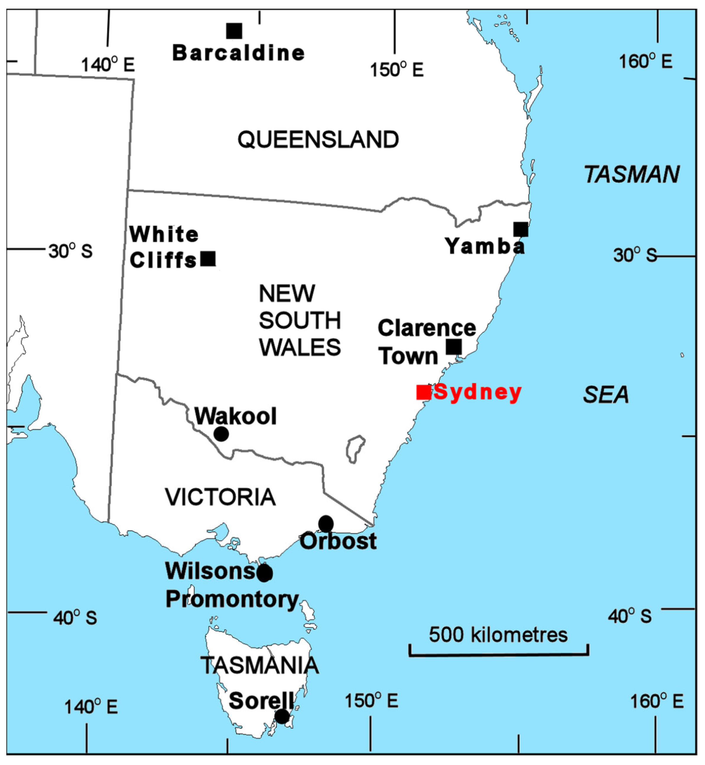
Figure 2.
(a) Australian rainfall deciles from 1 January 2017 to 31 December 2019; http://www.bom.gov.au/climate/maps/rainfall (accessed on 1 April 2024) (b) Australian rainfall deciles from 1 September 2019 to 31 August 2023; http://www.bom.gov.au/climate/maps/rainfall (accessed on 1 April 2024).
Figure 2.
(a) Australian rainfall deciles from 1 January 2017 to 31 December 2019; http://www.bom.gov.au/climate/maps/rainfall (accessed on 1 April 2024) (b) Australian rainfall deciles from 1 September 2019 to 31 August 2023; http://www.bom.gov.au/climate/maps/rainfall (accessed on 1 April 2024).
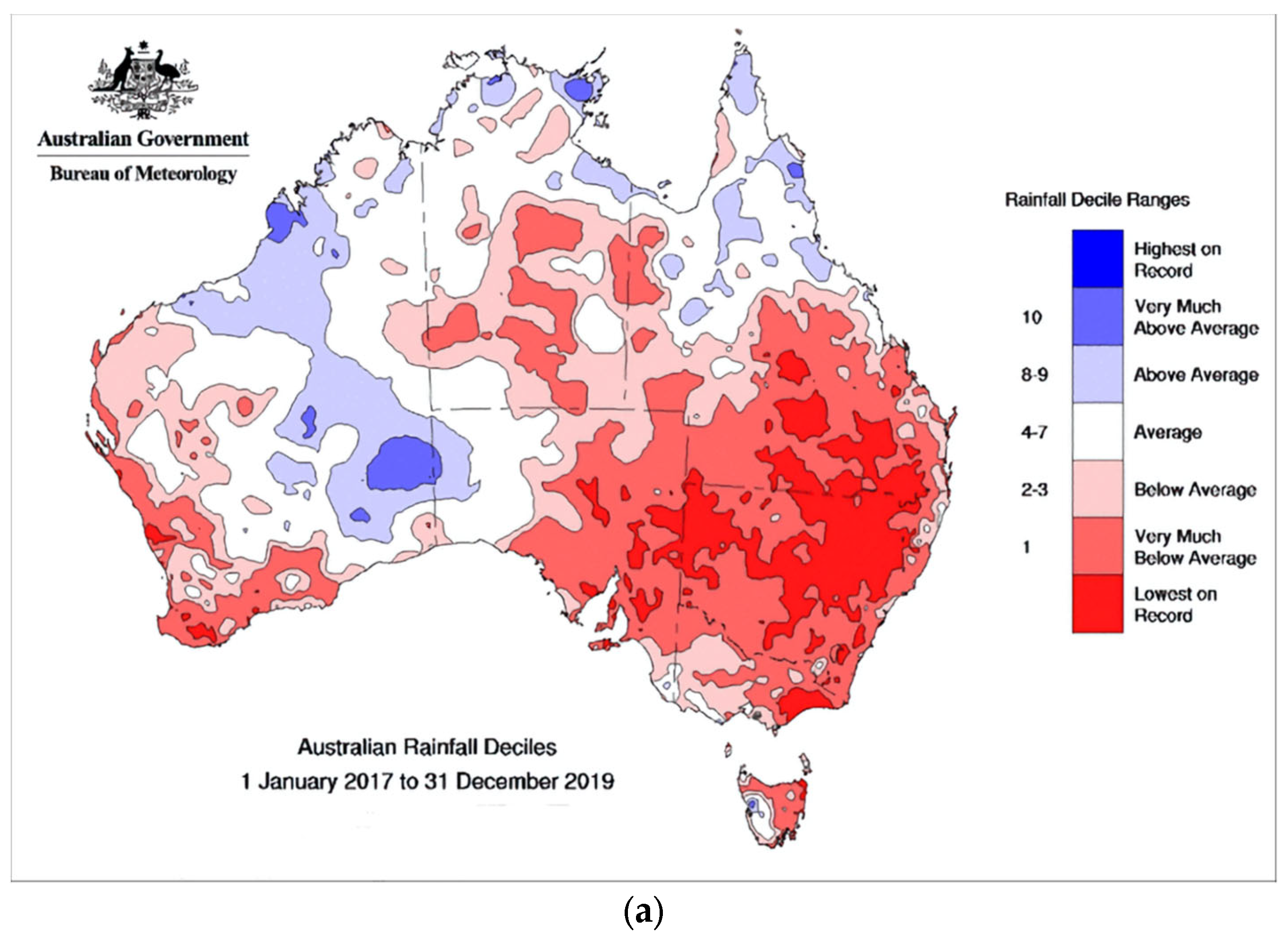

Figure 3.
The total precipitation and mean TMax time series for the 8 stations in SEAUS in the 1970–2022 period (a–h). The horizontal dashed lines indicate the 5th and 95th percentiles (red); 10th and 90th percentiles (orange); 15th and 85th percentiles (light green); 20th and 80th percentiles (brown); and 25th and 75th percentiles (dark blue). The horizontal solid black line is the median.


Figure 4.
The total precipitation and mean TMax time series for the 4 stations in N in the 1970–2022 period (a–h). The horizontal dashed lines indicate the 5th and 95th percentiles (red); 10th and 90th percentiles (orange); 15th and 85th percentiles (light green); 20th and 80th percentiles (brown); and 25th and 75th percentiles (dark blue). The horizontal solid black line is the median.

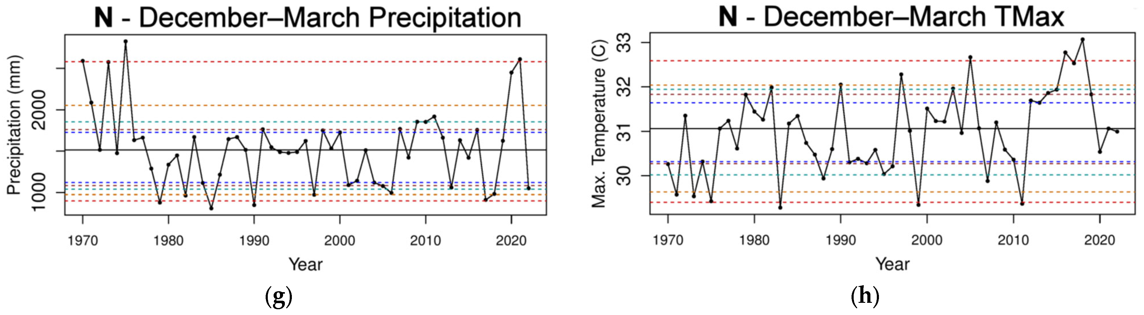
Figure 5.
The total precipitation and mean TMax time series for the 4 stations in S over the 1970–2022 period (a–h). The horizontal dashed lines indicate the 5th and 95th percentiles (red); 10th and 90th percentiles (orange); 15th and 85th percentiles (light green); 20th and 80th percentiles (brown); and 25th and 75th percentiles (dark blue). The horizontal solid black line is the median.


Table 1.
The p-values from the permutation testing differences in interval means and variances. The p-values for the permutation testing differences of the means and variances for total precipitation and TMax between the 1971–1996 and 1997–2022 periods. Significant p-values (≤0.10 and >0.05) are shown in italics. Highly significant p-values (≤0.05) are shown in bold italics.
| Area | Descriptive Statistic | p-Values for the Differences between the 1971–1996 and 1997–2022 Periods | |||||||
|---|---|---|---|---|---|---|---|---|---|
| Annual | April–May | July–November | December–March | ||||||
| Precip. | TMax | Precip. | TMax | Precip. | TMax | Precip. | TMax | ||
| SEAUS | Mean | 0.38 | 0 | 0.13 | 0.07 | 0.73 | 0 | 0.58 | 0 |
| Variance | 0.56 | 0.68 | 0.055 | 0.24 | 0.25 | 0.88 | 0.62 | 0.47 | |
| N | Mean | 0.98 | 0 | 0.19 | 0.05 | 0.25 | 0 | 0.83 | 0 |
| Variance | 0.54 | 0.48 | 0.36 | 0.55 | 0.39 | 0.65 | 0.91 | 0.42 | |
| S | Mean | 0.06 | 0 | 0.2 | 0.19 | 0.075 | 0 | 0.28 | 0 |
| Variance | 0.48 | 0.91 | 0.086 | 0.46 | 0.94 | 0.72 | 0.80 | 0.77 | |
Table 2.
p-values from the permutation testing differences of the interval means and variances for total precipitation between six quasi-decadal splits (each split 13 years) covering the 1971–2022 period. Significant p-values (≤0.10 and >0.05) are shown in italics. Highly significant p-values (≤0.05) are shown in bold italics.
| Area | Time of Year | Descriptive Statistic | 1971–1983 and 1984–1996 | 1971–1983 and 1997–2009 | 1971–1983 and 2010–2022 | 1984–1996 and 1997–2009 | 1984–1996 and 2010–2022 | 1997–2009 and 2010–2022 |
|---|---|---|---|---|---|---|---|---|
| SEAUS | Annual | Mean | 0.31 | 0.088 | 0.68 | 0.30 | 0.64 | 0.24 |
| Variance | 0.071 | 0.091 | 0.61 | 0.81 | 0.056 | 0.12 | ||
| April–May | Mean | 0.58 | 0.17 | 0.13 | 0.53 | 0.41 | 0.76 | |
| Variance | 0.70 | 0.079 | 0.44 | 0.073 | 0.285 | 0.37 | ||
| July–November | Mean | 0.73 | 0.64 | 0.82 | 0.31 | 0.98 | 0.52 | |
| Variance | 0.083 | 0.18 | 0.23 | 0.77 | 0.015 | 0.81 | ||
| December–March | Mean | 0.26 | 0.11 | 0.8 | 0.49 | 0.46 | 0.22 | |
| Variance | 0.15 | 0.21 | 0.68 | 0.67 | 0.090 | 0.21 | ||
| N | Annual | Mean | 0.11 | 0.21 | 0.76 | 0.69 | 0.26 | 0.43 |
| Variance | 0.66 | 0.68 | 0.31 | 0.94 | 0.28 | 0.22 | ||
| April–May | Mean | 0.78 | 0.57 | 0.11 | 0.82 | 0.23 | 0.27 | |
| Variance | 0.70 | 0.69 | 0.54 | 0.56 | 0.44 | 0.78 | ||
| July–November | Mean | 0.62 | 0.66 | 0.48 | 0.37 | 0.25 | 0.73 | |
| Variance | 0.92 | 0.69 | 0.49 | 0.71 | 0.51 | 0.60 | ||
| December–March | Mean | 0.20 | 0.16 | 0.87 | 0.87 | 0.23 | 0.20 | |
| Variance | 0.10 | 0.12 | 0.84 | 0.75 | 0.26 | 0.31 | ||
| S | Annual | Mean | 0.88 | 0.077 | 0.64 | 0.0088 | 0.43 | 0.15 |
| Variance | 0.042 | 0.033 | 0.31 | 0.8 | 0.091 | 0.26 | ||
| April–May | Mean | 0.39 | 0.046 | 0.53 | 0.24 | 0.74 | 0.075 | |
| Variance | 0.44 | 0.042 | 0.16 | 0.14 | 0.50 | 0.74 | ||
| July–November | Mean | 0.33 | 0.27 | 0.72 | 0.030 | 0.16 | 0.46 | |
| Variance | 0.50 | 0.52 | 0.90 | 0.64 | 0.17 | 0.50 | ||
| December–March | Mean | 0.80 | 0.26 | 0.70 | 0.26 | 0.58 | 0.58 | |
| Variance | 0.11 | 0.98 | 0.33 | 0.06 | 0.76 | 0.43 |
Table 3.
p-values from the permutation testing differences of interval means and variances for the mean TMax value between six quasi-decadal (13-year) splits covering the 1971–2022 period. Significant p-values (≤0.10 and >0.05) are shown in italics. Highly significant p-values (≤0.05) are shown in bold italics.
| Area | Time of Year | Descriptive Statistic | 1971–1983 and 1984–1996 | 1971–1983 and 1997–2009 | 1971–1983 and 2010–2022 | 1984–1996 and 1997–2009 | 1984–1996 and 2010–2022 | 1997–2009 and 2010–2022 |
|---|---|---|---|---|---|---|---|---|
| SEAUS | Annual | Mean | 0.31 | 0.0078 | 0.0028 | 0 | 0.0002 | 0.24 |
| Variance | 0.24 | 0.62 | 0.64 | 0.98 | 0.49 | 0.044 | ||
| April–May | Mean | 0.84 | 0.36 | 0.10 | 0.44 | 0.11 | 0.44 | |
| Variance | 0.36 | 0.62 | 0.58 | 0.28 | 0.35 | 0.77 | ||
| July–November | Mean | 0.78 | 0.019 | 0.011 | 0.0018 | 0.0014 | 0.51 | |
| Variance | 0.083 | 0.60 | 0.96 | 0.77 | 0.42 | 0.31 | ||
| December–March | Mean | 0.18 | 0.12 | 0.026 | 0.0036 | 0.001 | 0.25 | |
| Variance | 0.21 | 0.74 | 0.53 | 0.73 | 0.41 | 0.18 | ||
| N | Annual | Mean | 0.77 | 0.026 | 0.012 | 0.0038 | 0.005 | 0.35 |
| Variance | 0.31 | 0.76 | 0.54 | 0.79 | 0.37 | 0.067 | ||
| April–May | Mean | 0.89 | 0.38 | 0.16 | 0.27 | 0.078 | 0.44 | |
| Variance | 0.47 | 0.97 | 0.708 | 0.65 | 0.55 | 0.63 | ||
| July–November | Mean | 0.91 | 0.038 | 0.023 | 0.011 | 0.0078 | 0.51 | |
| Variance | 0.28 | 0.71 | 0.72 | 0.80 | 0.38 | 0.23 | ||
| December–March | Mean | 0.85 | 0.22 | 0.039 | 0.088 | 0.014 | 0.34 | |
| Variance | 0.043 | 0.83 | 0.86 | 0.29 | 0.25 | 0.64 | ||
| S | Annual | Mean | 0.13 | 0.008 | 0.0002 | 0 | 0 | 0.18 |
| Variance | 0.57 | 0.75 | 0.79 | 0.68 | 0.97 | 0.25 | ||
| April–May | Mean | 0.61 | 0.46 | 0.13 | 0.77 | 0.27 | 0.49 | |
| Variance | 0.83 | 0.48 | 0.68 | 0.59 | 0.79 | 0.81 | ||
| July–November | Mean | 0.67 | 0.018 | 0.0062 | 0.0004 | 0.0006 | 0.57 | |
| Variance | 0.12 | 0.90 | 0.55 | 0.89 | 0.91 | 0.93 | ||
| December–March | Mean | 0.035 | 0.27 | 0.048 | 0.0058 | 0.001 | 0.29 | |
| Variance | 0.90 | 0.68 | 0.66 | 0.80 | 0.77 | 0.79 |
Table 4.
The five attributes for each area and monthly group consisting of greater than or equal to 50% mean folds across the eight ML methods using a sliding training window with a size of 20 and a fixed testing window with a size of 20. †,# indicate an equal mean value.
Table 4.
The five attributes for each area and monthly group consisting of greater than or equal to 50% mean folds across the eight ML methods using a sliding training window with a size of 20 and a fixed testing window with a size of 20. †,# indicate an equal mean value.
| Area of SEAUS | Annual | April–May | July–November | December–March |
|---|---|---|---|---|
| SEAUS | AMO*PMM Niño3.4 PMM*TPI AMO*IOD † AMO*TSSSTA † | AMO*TSSSTA IOD*PMM SAM GlobalSSTA*PMM Niño3.4 † IOD*SAM † | Nino3.4 IOD SOI PMM*TPI TPI † Niño3.4*TPI † | IOD*SAM PMM*SAM IOD*Niño3.4 GlobalSSTA † Niño3.4*SOI † PMM*SOI † |
| N | SOI PMM Niño3.4 Niño3.4*SOI † Niño3.4*TPI † | AMO*PMM Niño3.4 IOD*PMM IOD*Niño3.4 SAM | SAM TPI Niño3.4 SOI AMO*SAM | IOD*SAM PMM*TPI AMO*SAM † Niño3.4*SOI † SAM*TSSSTA † |
| S | IOD IOD*SAM SOI*TSSSTA AMO*IOD GlobalSSTA † Niño3.4*TPI † | AMO*TSSSTA Niño3.4*PMM † IOD*Nino3.4 † AMO*IOD AMO*PMM # AMO*TPI # PMM # IOD*SAM # | IOD AMO # AMO*PMM SOI † TSSSTA † IOD*Niño3.4 † PMM*SAM # SOI*TSSSTA † | SOI*TSSSTA AMO*GlobalT AMO*PMM † TPI † TPI*TSSSTA † |
Disclaimer/Publisher’s Note: The statements, opinions and data contained in all publications are solely those of the individual author(s) and contributor(s) and not of MDPI and/or the editor(s). MDPI and/or the editor(s) disclaim responsibility for any injury to people or property resulting from any ideas, methods, instructions or products referred to in the content. |
© 2024 by the authors. Licensee MDPI, Basel, Switzerland. This article is an open access article distributed under the terms and conditions of the Creative Commons Attribution (CC BY) license (https://creativecommons.org/licenses/by/4.0/).
Share and Cite
MDPI and ACS Style
Speer, M.; Hartigan, J.; Leslie, L. The Machine Learning Attribution of Quasi-Decadal Precipitation and Temperature Extremes in Southeastern Australia during the 1971–2022 Period. Climate 2024, 12, 75. https://doi.org/10.3390/cli12050075
AMA Style
Speer M, Hartigan J, Leslie L. The Machine Learning Attribution of Quasi-Decadal Precipitation and Temperature Extremes in Southeastern Australia during the 1971–2022 Period. Climate. 2024; 12(5):75. https://doi.org/10.3390/cli12050075
Chicago/Turabian StyleSpeer, Milton, Joshua Hartigan, and Lance Leslie. 2024. "The Machine Learning Attribution of Quasi-Decadal Precipitation and Temperature Extremes in Southeastern Australia during the 1971–2022 Period" Climate 12, no. 5: 75. https://doi.org/10.3390/cli12050075
Note that from the first issue of 2016, this journal uses article numbers instead of page numbers. See further details here.