Frictional Behavior of Chestnut (Castanea sativa Mill.) Sawn Timber for Carpentry and Mechanical Joints in Service Class 2

Abstract

Wood is poised to become a material of choice for future construction. When appropriately managed, it is a renewable material with unique mechanical properties. Thus, there has been a growing demand for hardwoods, including Castanea sativa Mill., the focal point of this investigation, for structural applications. Albeit in a limited capacity, Eurocode 5-2 offers friction coefficients for softwoods, but it falls short for hardwoods. These coefficients play a critical role in numerical simulations involving friction, enabling the optimization of joints and, by extension, the overall structural integrity. Test samples were evaluated at 15% and 18% moisture content (Service Class 2) for various orientations of timber-to-timber and timber-to-steel friction. The results provide an experimental database for numerical simulations and highlight the influence of moisture on the stick–slip phenomenon, which was absent for the timber-to-timber tests, as well as on the rising friction values. At 18%, the static and kinetic coefficients were 0.70 and 0.48 for timber-to-timber and 0.5 and 0.50 for timber-to-steel. The increase was around 50% for timber-to-timber friction and over 170% for timber-to-steel pairs. Moreover, the findings proved a relationship between both coefficients and the validity of the linear estimation approach within the 12–18% moisture commonly applied to softwoods.

1. Introduction

Historically, wood has been a traditional and widely used material in construction due to its abundance, ease of use, and adequate mechanical properties. However, as technological advancements made steel and concrete not only more accessible but also cost-effective, these materials began to be perceived as superior alternatives due to their modern aesthetic, enhanced durability, and significantly improved fire resistance. In turn, the prominence of wood in the construction industry diminished as it was relegated to small-scale or less demanding structural applications due to concerns regarding instability, fire safety, decay, and sound transmission [1].

Currently, with the construction sector widely recognized as a major contributor to environmental degradation due to substantial material and energy consumption, greenhouse gas emissions, and waste generation, wood is experiencing a resurgence as a sustainable construction material. The favorable mechanical properties relative to its weight, the enhancement of its durability through innovative treatments, and the advent of new engineered timber products, e.g., glued laminated timber (glulam), cross-laminated timber (CLT), and laminated veneer lumber (LVL), are some of the driving factors in its resurgence besides the pursuit of sustainable development. In this regard, beyond its inherent sustainability, the use of wood has a crucial role in addressing climate change concerns due to its significantly lower embodied energy [2] and reduced CO₂ emissions [3,4] while simultaneously acting as a carbon sink of approximately 1.5 t of CO₂ per m³ of wood [5]. As a renewable resource originating from responsibly managed forests, wood further alleviates the pressures of raw material scarcity, highlighting its multifaceted contribution to environmental conservation.

For this investigation, chestnut wood (Castanea sativa, Mill.) was selected as this deciduous species covers more than 2.5 million hectares in Europe around the Mediterranean region, with 89% concentrated in France, Italy, Spain, Portugal, and Switzerland, in decreasing order of importance, as shown in Figure 1 [6]. Several research works have underscored its ecological relevance as a source of support for a wide variety of flora and fauna [7,8] and the European Council has included “9260 Castanea sativa woods’” in Annex 1 of the Habitats Directive [9]. Commercially, chestnut is valued both for fruit and non-wood products as well as timber. For instance, in Spain, the average total volume (with bark) of chestnut stands harvested in 2021 reached 97,878 m³ [10], mostly from the north provinces (Galicia, Asturias, Navarre, and Catalonia), but also arising from the center and south of the country (Figure 1). Chestnut wood is valued for its appearance and strength; it is particularly appreciated for external use due to its natural protection against decay [11,12], and it possesses a vast tradition of use for both structural and non-structural purposes in construction (beams, joists, and traditional grain stores), woodworking, furniture, flooring, fine veneer, general joinery, and poles) [11]. Nowadays, sustainability concerns have spurred a new interest in its use. In this regard, Carbone et al. [13], who investigated the market competitiveness of laminated chestnut timber products, forecasted a bright future for this type of wood while indicating the need for a targeted chestnut wood policy to significantly bolster its market penetration and growth.

In structural timber engineering, the friction properties of wood, which are the focus of this study, hold significant relevance, particularly in the designing of joints and supports. The friction coefficient between wooden parts or between wood and metal connectors significantly influences the magnitude and manner of force transmission [14,15,16,17,18,19,20]. For instance, in step joints [14] and reverse joints [18], load distribution varies across contact faces depending on the coefficient of friction. For tie-rafter connections in trusses, a higher friction coefficient increases force transmission in areas of greater contact while reducing it in areas of lesser contact, thus decreasing the shear stress at the tie end and increasing the compression oblique to the grain in the rafter. For dowel joints [15], a higher friction coefficient leads to a more uniform stress distribution around the perimeter, which reduces joint slippage. In tapered tenon joints [16,17], the friction coefficient affects the forces on the frontal and lateral faces differently, with a higher friction coefficient reducing the contact forces on the front face. For connections with dowel-type fasteners and nut–washer fixings [19], the pre-tensioning creates an initial axial load that improves the friction effect at the wood–wood interfaces and the load distribution between faces. For timber connections with metal fasteners [20], the friction coefficient impacts the distribution of loads transmitted directly between pieces, whether through metal–wood or wood–wood contacts.

Thus, the understanding of this parameter is crucial for the analysis and simulation of both carpentry joints and mechanical connections. As with most mechanical properties of wood, friction also varies with the moisture content reached by the specimen in balance with the relative humidity and temperature of its surrounding environment. Consequently, Eurocode 5 [21] incorporates this effect in design by establishing three service classes reflecting the environmental conditions (i.e., temperature and relative humidity of the surrounding air) to which the wood will be exposed and its eventual equilibrium moisture content:

• Service Class 1: corresponds to conditions (20 °C and 65% relative humidity) where the average moisture content in most softwoods remains below 12%;
• Service Class 2: corresponds to conditions (20 °C and 85% relative humidity) where the average moisture content in most softwoods remains below 20%;
• Service Class 3: corresponds to conditions where the average moisture content in most softwoods exceeds 20%.

It should be noted that although Eurocode 5 [21] identifies service classes for softwoods, the temperature and relative humidity conditions describing the different service classes and moisture contents are also applicable to hardwoods such as chestnut. In this regard, there are international standards that define service classes applicable to both softwood and hardwood. For instance, the National Design Specification for Wood Construction [22] issued by ANSI defines two service conditions: “dry” (with up to 16% moisture content for laminated wood and CLT and 19% for sawn wood) and “wet” (for moisture contents exceeding these levels). Likewise, the Canadian standard for engineering design in wood [23] specifies a “dry” service condition, where the average equilibrium moisture content of solid wood over a year is 15% or less and does not exceed 19%, whereas the “wet” service condition encompasses all conditions that do not meet the dry criteria.

Therefore, the standards used to characterize the mechanical properties of wood stipulate testing at a specific moisture level, commonly 12%. Then, subsequent adjustments are made in calculations through the use of coefficients based on the intended service class. However, there is no European standard regarding the experimental determination of friction coefficients, but conversely, it is referenced in Table 6.1 of Eurocode 5-2 [24] for conifer timber in the context of stress-laminated decks. Specifically, values for the static friction coefficient are provided at moisture contents of ≤12% and ≥16%, with the provision that values within this range can be linearly interpolated.

Although several researchers [25,26,27] have commented on the linear variation in properties with moisture contents from 8% to 20%, or until fiber saturation is reached, limited research has explored the relationship between moisture content variations and friction, with investigations predominantly centered at the 12% equilibrium moisture content. Among those that do consider or provide insights on moisture content, the following studies (

Table 1. Noteworthy fiction coefficients from the literature review.

Test	Static Friction Coefficient	Kinetic Friction Coefficient	Moisture Content	References
Timber-to-timber	0.25 to 0.7	0.15 to 0.4	Dry	Argüelles et al. [26,28]
Timber-to-timber	0.5 to 0.71	0.3 to 0.65	From 11.25% to 20% at different wood sections (tangential, diagonal, and radial)	Fu et al. [29]
Timber-to-timber	0.36 to 052	0.25 to 0.34	12% at different orientation of the contact surfaces	Villar-García et al. [30]
Timber-to-timber	0.44 to 0.51	0.33 to 0.39	12% at different orientation of the contact surfaces	Villar-García et al. [31]
Timber-to-steel	-	0.1 to 0.3	From 10% to 14%	McKenzie et al. [32]
	-	0.4 to 0.64	At fiber saturation
Timber-to-steel	-	0.3 to 0.5	Dry	Glass and Zelinka [27]
	-	0.5 to 0.7	Intermediate moisture
	-	0.7 to 0.9	Close to saturation
Timber-to-steel	0.156 to 0.238	-	12% at different fiber directions	Dorn et al. [33]
	0.121 to 0.176	-	Oven-dried at different fiber directions
	0.280 to 0.344	-	Saturated at different fiber directions
Timber-to-steel	0.16 to 0.21	0.15 to 0.18	12% at different orientations of the contact surfaces	Villar-García et al. [31]

) are noteworthy.

For varying moisture content values, Argüelles et al. [26,28] reported values for the static friction coefficient ranging from 0.25 to 0.7 and for the kinetic friction coefficient within the 0.15 to 0.4 range. The coefficients increased with the moisture content of the timber-to-timber testing specimen up to saturation and remained constant beyond that point. This effect was also noticed by Glass and Zelinka [27], who reported that the coefficients continuously increase until fiber saturation is reached. Then, the values stabilize until water is present on the surface, triggering a decrease in the coefficients due to the lubricating effect. Although for beech timber, Fu et al. [29] examined the influence of both the moisture content and wood section (i.e., tangential, diagonal, and radial) on the static and kinetic friction coefficients. Both values increased with the moisture content within the 5–30% range, but greater moisture contents are responsible for marginal increases. For the different orientations of the contact surfaces, the authors reported static friction coefficients ranging from 0.5 to 0.71 and kinetic friction coefficients ranging from 0.3 to 0.65 at 11.25% and 20% moisture levels, respectively.

Regarding timber-to-steel friction, there are a limited number of studies, predominantly focused on dynamic assessments. McKenzie et al. [32] performed an extensive examination of the kinetic friction coefficients of numerous wood species against rough and smoot steel surfaces, although chestnut was not included in the investigation. For smooth surfaces, which are common in timber connections, the study reported kinetic friction coefficients ranging from 0.1 to 0.3 for moisture contents between 10% and 14%, depending on the speed of sliding. For moisture levels at fiber saturation, the values ranged from 0.4 to 0.64 for increasing sliding speeds. Moreover, based on the figures describing the dynamic friction included in the research, it could be inferred that the static friction values were only slightly higher than those reported for the kinetic friction.

Similarly, Glass and Zelinka [27] noticed that the kinetic friction coefficient for smooth timber in contact with hard, smooth surfaces, such as steel, can vary from 0.3 to 0.5 in dry specimens, from 0.5 to 0.7 at intermediate moisture contents, and from 0.7 to 0.9 when approaching saturation. Despite the distinct properties compared to sawn timber, it is worth mentioning the study on the friction behavior of microlaminated Picea abies against steel carried out by Dorn et al. [33]. The authors recorded static friction coefficient values ranging between 0.16 and 0.24 at a 12% moisture content. For oven-dried specimens, these values remained mostly constant. However, for saturated specimens, the static friction coefficient increased between 74% to 123% for tests parallel to the grain and between 82% and 182% for tests perpendicular to the grain.

This research focuses on the study of both static and kinetic friction coefficients of chestnut timber. Through an enhanced understanding of friction, the aim is to expand the use of Castanea sativa for structural designs involving frictional forces, promoting construction sustainability by encouraging the use of less exploited materials, which entails a diversification in the range of species used in construction and thus alleviates the demand for more commonly exploited ones. Examples of targeted applications include stressed plate bridges and walkways, timber trusses with carpentry joints, and constructions with mechanical timber-to-steel connections. The experimental program takes into account the orthotropic nature of wood by assessing different wood orientations involving both the wooden frictional pairs as well as against a steel plate. Moreover, the influence of the moisture content was considered by carrying out tests at 15% and 18% (i.e., Service Class 2 conditions). The results arising from the experimental program would provide a comprehensive database to be used as an input for precise engineering calculations, such as those carried out in numerical simulations, that would allow for a more accurate volumetric optimization of this natural resource. Additionally, in combination with previous findings by the authors on timber-to-timber and timber-to-steel tests at a 12% moisture content [30,31], this program would be used to validate the interpolation approach suggested for softwoods within the 12–18% moisture content range for hardwoods.

2. Materials and Methods

Test samples of 105 × 50 × 25 mm were prepared from Spanish chestnut (Castanea sativa Mill.) with a density of 670 kg/m³ (12% moisture content). Since the variation in moisture content changes the frictional properties of wood, the tests were carried out at two moisture contents: firstly, at 18% moisture content, which represents Service Class 2 according to Eurocode 5 [21] (e.g., structures under cover but open to the air, canopies, covered pergolas, walkways, and bridges that are either covered or protected by a wear layer, as well as indoor and enclosed swimming pools [21,25,26]), then at 15% moisture content (i.e., an intermediate value to the 12% moisture content used to represent the conditions of Service Class 1 established in Eurocode 5 [21]). Thus, one set of specimens was stored in a condition room with a constant temperature of 20 °C and a relative humidity of 85% to ensure hygroscopic equilibrium and the desired moisture content of 18%. Conversely, for conditioning to a humidity of 15%, a temperature of 38 °C and a humidity of 80% were set [27]. The moisture levels were checked immediately before carrying out the tests using a hygrometer and afterwards via oven drying according to EN 13183-1 [34].

In the absence of a specific European standard test for determining the friction coefficient of wood and drawing upon the general recommendations provided by the American standard ASTM G115-10 [35], the authors developed and validated a test procedure based on a direct shear machine [36]. The proposed method adapts common geotechnical equipment to facilitate the placement and contact of the surfaces to be tested (i.e., specimens were positioned in the device by their largest surface area, ensuring that sliding occurred along the longest dimension), thereby facilitating both accurate experimental conditions as well as the application and recording of the necessary variables. Firstly, this method allows for the application of a normal load (N) to the upper face of the specimen through a distribution plate connected to a load bridge and counter-balance device while controlling the sliding speed. Similar to other research works [30,31,37,38], this study employed a 0.5 MPa load and an 8 mm·min⁻¹ speed to simulate conditions encountered in practice while also effectively preventing the occurrence of inertial forces. Moreover, this method enables the measurement of both displacement and the necessary force (F) required to produce sliding by means of an LVDT (Linear Variable Differential Transformer) displacement sensor and load cell sensor, respectively. Therefore, the coefficient of friction (μ) is determined according to Equation (1):

F = μ × N,

(1)

Here, the proportionality constant is the friction coefficient, designated as either the static friction coefficient (μ_s) or kinetic friction coefficient (μ_k), contingent upon whether it pertains to the value at the precise moment just before sliding commences or during the ongoing relative displacement of the solids or the surfaces under examination.

Two separate experimental series were executed to evaluate the frictional behavior between pairs of materials: one set examined timber-to-timber interactions while the other focused on timber-to-steel contacts. Moreover, to simulate the conditions of surfaces that are designed to come into contact within the joint assembly, the influence of both the orthotropic nature of wood as well as the different roughness across the cutting planes was considered. As such, three distinct orthogonal axes were considered: longitudinal -L- (parallel to the fiber or grain, i.e., the axis of the tree), radial -R- (perpendicular to the grain in the radial direction and normal to the growth rings), and tangential -T- (perpendicular to the grain but tangent to the growth rings), as shown in Figure 2.

Consequently, the three possible friction planes and their two respective directions of slippage were evaluated (Figure 2), ensuring a comprehensive analysis of frictional behavior under varied conditions:

• Transverse plane (perpendicular to the fiber):

• (A) predominant direction of radial sliding (sliding parallel to the radius of the growth rings);
• (B) predominant direction of tangential sliding to the growth rings;

• Radial plane (defined by the axis of the three and a radius of the trunk):

• (C) sliding direction parallel to the fiber (i.e., radial surfaces);
• (D) sliding direction perpendicular to the fiber;

• Tangential plane (tangent to the growth rings):

• (E) sliding direction parallel to the fiber (i.e., tangential surfaces);
• (F) sliding direction perpendicular to the fiber.

Therefore, Figure 2 presents the array of friction pairs that reflect combinations frequently encountered in structural connections. On the one hand, timber-to-timber tests could be divided among surfaces with identical orientations: A-A, B-B, C-C, D-D, E-E, and F-F, and tests between surfaces of differing orientations: A-C, A-E, B-C, and B-E. On the other hand, timber-to-steel tests were designed as A-S, B-S, C-S, D-S, E-S, and F-S, with S indicating the steel plate. Thus, the experimental program reached a total of over 400 tests and ultimately offered significant insights into frictional behavior.

3. Results and Discussion

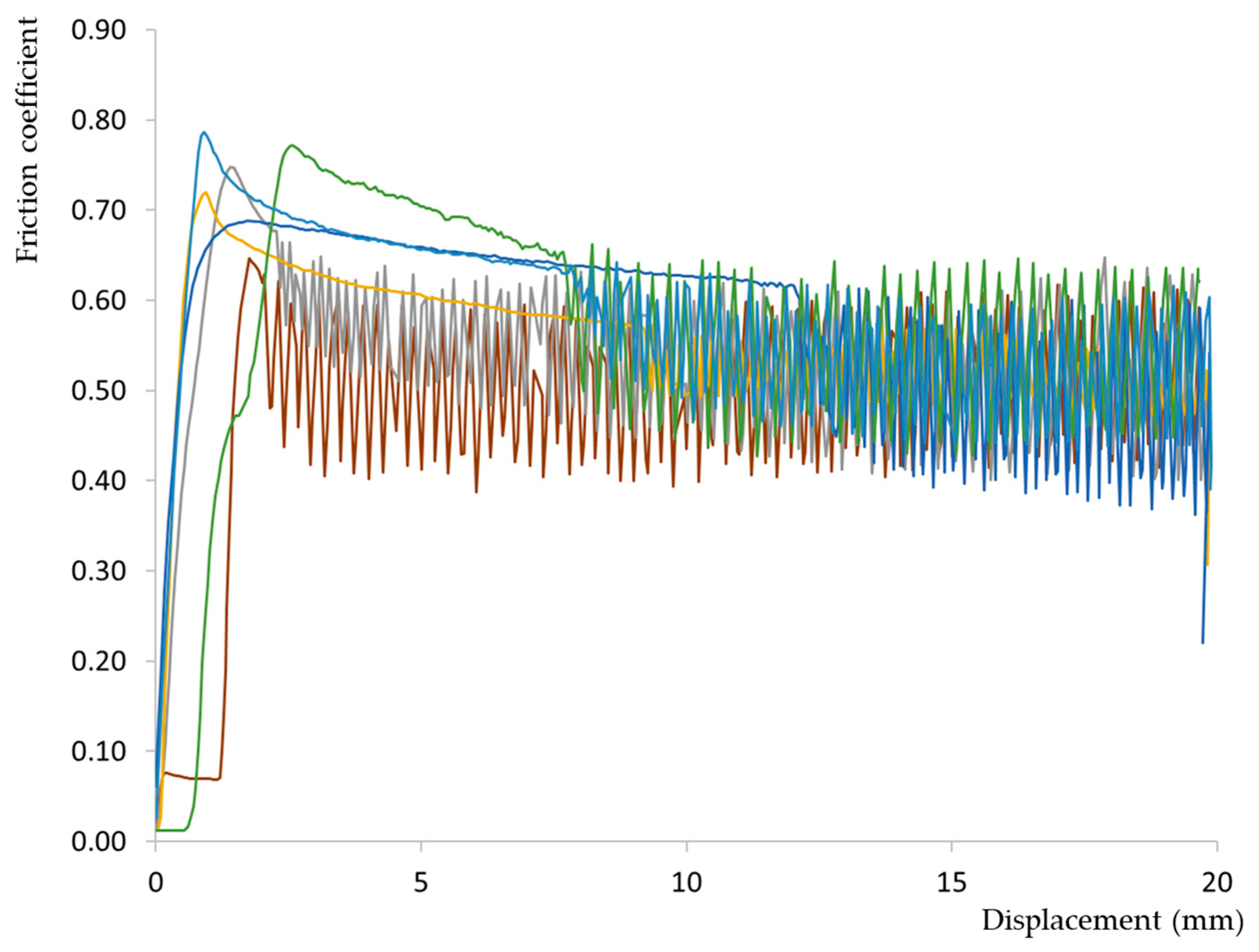
3.1. Timber-to-Timber Tests with Identical Orientations

Figure 3 showcases the most illustrative graphs depicting the variation of the friction coefficient relative to the displacement for tests involving surfaces of identical orientations and friction directions under a controlled moisture content of 18%.

The oscillations observed in Figure 3 are illustrative of the stick–slip phenomenon. However, the fluctuation manifested with reduced intensity compared to similar tests conducted at lower moisture levels [30,31]. This reduction aligns with findings by [29,39], highlighting that higher moisture weakens the stick–slip behavior between the wood surfaces. The differences between the frictional force–displacement curves of dry and wet surfaces were also observed by Fu et al. [29], who attributed them to the softening of the fibers and the decreased amplitude of the rough peaks, which led to a weakened stick–slip motion in the 5–30% moisture range. As described by Möhler and Herröder [40] in friction scenarios A and C, the sliding motion occurs continuously across the friction path and is characterized by a parabolic decrease in the horizontal force, at least in an initial segment.

Table 2. Friction coefficients between wood surfaces of identical orientation at 18% moisture content.

Mean (CoV %)	A-A	B-B	C-C	D-D	E-E	F-F
μs	0.67 (15.3)	0.71 (11.4)	0.68 (14.4)	0.78 (8.2)	0.63 (13.9)	0.73 (9.9)
μk	0.42 (4.8)	0.47 (12.7)	0.49 (12.9)	0.56 (16.7)	0.46 (29.3)	0.54 (24.6)

shows the friction coefficients from various sawn specimens and frictional directions grouped by friction pairs with identical orientations and a moisture content of 18%. Both the mean value derived from the 15 tests performed for each specific pairing and the coefficient of variation (CoV) are indicated to highlight the average performance and the variability within each set.

Based on the comparison between the results presented in Table 2 and those obtained for these same orientations in a previous work [30], it becomes noticeable that moisture content significantly impacts both static and kinetic friction, overshadowing the effects of the testing orientation. This finding aligns with observations made by [29]. Nonetheless, knowledge of the specific friction values for different wood orientations can significantly enhance decision making during joint construction. Then, it would allow for more favorable designs by tailoring the cut of wood, notches, and contact interfaces to optimize frictional force transmission between the components. By strategically exploiting the orthotropic nature of wood, such as by rotating the R and T axes of the beams, the distribution of stresses could be improved.

On average, disregarding orientation, the static friction coefficient stands at 0.70 and the kinetic friction coefficient at 0.48. Such values represent roughly 50% increases compared to those measured at 12% moisture content. These findings are consistent with those reported by Argüelles et al. [26] (i.e., a 0.7 static friction coefficient and 0.4 kinetic friction coefficient) and Fu et al. [29] at 20% moisture content (μ_s = 0.5–0.71; μ_k = 0.3–0.65). In this experimental program, the average coefficients of variation for the different orientation test series were 7.6% for static friction and 10% for kinetic friction. Notably, the CoV for each friction pair significantly decreased by about 15% compared to the 12% moisture tests, suggesting that increased moisture on the contact surfaces leads to less variability in friction.

3.2. Timber-to-Timber Tests with Different Orientations

Figure 4 presents some representative examples that capture the fluctuation of the friction coefficient as a function of displacement, focusing on experiments that involve surfaces with different orientations and sliding directions, conducted at a moisture content of 18%.

Similar observations apply to Figure 4 regarding the stick–slip behavior of the tested specimens. The performance of the friction pairs demonstrates a consistent relationship between the displacement and friction coefficient, closely aligning with the patterns noted in scenarios of identical orientation between wood surfaces (Figure 3).

Table 3. Friction coefficients between wood surfaces of different orientations at 18% moisture content.

Mean (CoV %)	A-C	A-E	B-C	B-E
μs	0.70 (18.1)	0.65 (15.6)	0.64 (9.9)	0.70 (10.3)
μk	0.48 (25.7)	0.45 (13.6)	0.43 (14.3)	0.50 (20.7)

compiles the friction coefficients from various sawn specimens and frictional directions, grouped by friction pairs with identical orientations and a moisture content of 18%. A trend consistent with the earlier discussion is observed as values exhibit a notable increase compared to those at 12% moisture content [31]. Specifically, there is a 42% surge in the static friction coefficient, averaging at 0.67, and a 30% rise in the kinetic friction coefficient, averaging at 0.47. Nevertheless, the increment is less pronounced than the increase observed for samples with identical orientations, as recorded in Table 2.

The overall average values, both static and kinetic, are remarkably similar to those obtained for the same orientation at 18% moisture content and align with the referenced literature from the previous section. The lack of significant variance for any specific pair could respond to a homogenizing effect of increased moisture levels. Notably, the A-C and B-E pairings continue to register the greatest friction values, a pattern consistent with observations at 12% moisture. However, no direct correlation is observed between the highest values in Table 3 and the superior frictional values arising from the friction of wood surfaces of identical orientations (Table 2). Regarding the coefficient of variation, the values decreased compared to the 12% moisture level for each tested friction pair, mirroring the trend observed for pairs of identical orientation. Nonetheless, the CoV values remained in the same range as those obtained for 18% moisture content for wood surfaces of identical orientation.

It is worth noting that the average static friction coefficient value (μ_s = 0.69) significantly exceeds those specified in Eurocode 5-2 [24]. For the calculation of stress-laminated deck plates consisting of sawn softwood at a moisture content greater than 16%, the design values established for the static friction coefficient are 0.45 for scenarios perpendicular to grain and 0.35 for scenarios parallel to grain. Nevertheless, this comparison should take into account the case-specificity differences regarding the type of wood and moisture content (i.e., specimens derived from Castanea sativa, a deciduous tree, conditioned at 18% moisture content). Moreover, it should be acknowledged that the values stipulated by Eurocode 5-2 [24] serve as design guidelines, factoring in safety margins to ensure structural integrity. Thus, the proposed values in Eurocode 5-2 [24] are deliberately conservative since greater friction coefficient values are beneficial for the outcomes of the engineering calculations.

3.3. Timber-to-Steel Tests

Figure 5 showcases representative friction cases of the tests comparing the timber specimens at 18% moisture content and the steel plate, focusing on experiments that involved different fiber orientations relative to the sliding direction.

Conversely to previous timber-to-timber test series, Figure 5 illustrates the absence of the stick–slip phenomenon, corroborating findings from other studies [29,41]. As also noted by those researchers, the increase in moisture does not introduce a pronounced inflection at the beginning of displacement. The shape of the obtained curves (Figure 5) is similar to the type B classification proposed by Möhler and Herröder [40] in which the frictional force exhibits a flat parabolic shape, indicative of a friction trajectory that either slightly decreases or, in certain instances, remains constant after reaching the peak load. Notably, in some instances, the value of friction marginally increases shortly after the sliding begins.

Table 4. Friction coefficients involving a wood surface at 18% moisture content and the steel plate.

Mean (CoV %)	A-S	B-S	C-S	D-S	E-S	F-S
μs	0.48 (2.5)	0.49 (6.1)	0.55 (4.6)	0.53 (3.2)	0.54 (4.9)	0.52 (4.4)
μk	0.45 (7.2)	0.47 (7.2)	0.53 (7.2)	0.52 (3.1)	0.53 (5.2)	0.50 (5.3)

details the mean values for both static and kinetic friction coefficients, accompanied by the coefficient of variation from tests involving the interaction between a steel plate and a wood specimen conditioned at 18% moisture content and sawn to exhibit a specific orientation.

Analysis of the data in the test series for the different wood orientations reveals an average static friction coefficient of 0.52 and a kinetic friction coefficient of 0.50, with coefficients of variation of 6% and 7%, respectively. Two main insights emerge from these findings.

On the one hand, there is a substantial increase in both static and kinetic friction coefficients compared to steel–wood pairs at 12% moisture content [31]. For instance, the average static coefficient exhibits a 173% rise and the kinetic coefficient a 194% surge, which closely places the kinetic value on par with the static coefficient. The greater increase in the kinetic coefficients is indicative of a more pronounced effect of moisture that facilitated the lifting of the wood fibers during sliding interactions [29]. These substantial increases are in line with those documented by Dorn et al. [33], who conducted tests on wood against steel ranging from oven-dried to fully saturated specimens. Moreover, the obtained values fall within the range specified by Glass and Zelinka [27] for the friction of wood against hard and smooth surfaces at intermediate moisture (μ_k = 0.5–0.7) and are consistent with the findings reported by McKenzie et al. [32] of μ_k = 0.4–0.64. Nonetheless, it is worth noting that this increase significantly exceeds that observed for the same moisture variation in the timber-to-timber tests, suggesting that when friction occurs against a very smooth surface, such as steel, the moisture content of the wood has a significantly major role in the friction coefficient.

On the other hand, the CoV values within each orientation are considerably lower compared to those obtained for wood specimens at 12% moisture content. Such a reduction in variability is attributed to both the increased moisture at the contact surface and the homogenizing effect of steel (i.e., the limited roughness) in the wood–steel friction dynamics.

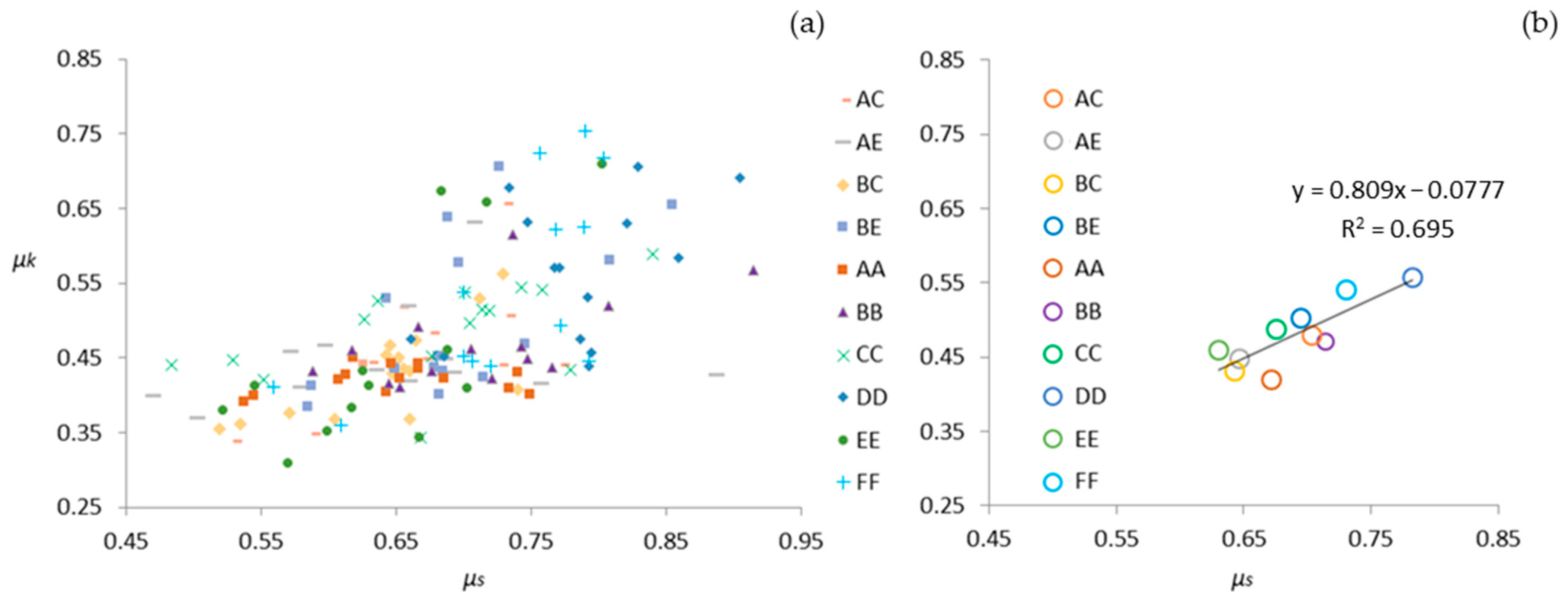
3.4. Correlation between μ_k and μ_s

For each friction specimen pairing within the timber-to-timber test series, Figure 6a illustrates the relationship between the static friction coefficient (μ_s) and the kinetic friction coefficient (μ_k). Similarly, Figure 6b displays the average values for each friction combination. The μ_k/μ_s ratio for surfaces of identical orientation averaged 0.72, similar to the values obtained at 12% moisture content, which indicated no significant change in their relationship. For surfaces of different orientations, the μ_k/μ_s ratio was 0.69, yielding a value comparable to that of surfaces with identical orientation at an 18% moisture level. This similarity suggests that the orientation of wood surfaces does not markedly affect the relationship between static and kinetic friction coefficients under the same moisture conditions.

Although no strong relationship emerged from the entire dataset, the analysis of the average values (Figure 6b) allowed for an acceptable correlation (R² = 0.70) between static and kinetic friction coefficients (Equation (2)).

μ_k = 0.809μ_s − 0.0777 (R² = 0.70),

(2)

Additionally, the consideration of specific friction orientations allowed for improved correlations such as those shown in Equations (3) and (4) for the A-C and E-E friction pairs, respectively.

For the friction pair A-C: μ_k = 0.98μ_s − 0.19 (R² = 0.76),

(3)

For the friction pair E-E: μ_k = 0.89μ_s − 0.035 (R² = 0.74),

(4)

A similar approach for the relationship of the static and kinetic friction coefficients of the timber-to-steel tests is followed in Figure 7a,b. The μ_k/μ_s ratio averages 0.97, which numerically captures the behavior depicted in Figure 5 (i.e., a flat parabolic curve with a minimal reduction in the coefficient value during sliding). In this case, a notable difference is observed in the ratio compared to the values obtained at 12% moisture, which had an average of 0.83, indicating a further reduction in the differences between static and kinetic values. The greater proximity to unity reflects the absence of the initial inflection point in the registered friction behavior. This phenomenon was also noted by Fu et al. [29], who observed that the difference between μ_s and μ_k decreases with higher moisture contents.

From the average coefficients for the different timber-to-steel tests, Equation (5) shows the relationship between static and kinetic friction. The robustness of the correlation (R² = 0.96) allows for a highly reliable prediction of the kinetic coefficient from a known static coefficient and vice versa. Moreover, the specific friction pair combinations also display strong correlations between both coefficients. It should be noted that the high degree of correlation was also identified for the 12% moisture content [31] pointing to a generalization of this observation across the entire studied moisture spectrum, as further detailed in subsequent discussions.

μ_k = 1.350μ_s − 0.199 (R² = 0.96),

(5)

3.5. Influence of Moisture Content on Friction Coefficients

To evaluate the validity of the linear coefficient–moisture relationships, the experimental program included a targeted series of tests at an intermediate moisture level of 15% while maintaining all other test parameters at constant levels. The average value and coefficient of variation from 10 determinations within each friction pair combination (i.e., between wood surfaces of identical orientation, wood surfaces of different orientations, and wood and steel) of static and kinetic coefficients are displayed in

Table 5. Friction coefficients between wood surfaces of identical orientation at 15% moisture content.

Mean (CoV %)	A-A	B-B	C-C	D-D	E-E	F-F
μs	0.59 (6.3)	0.61 (5.2)	0.51 (33.1)	0.69 (31.1)	0.48 (7.5)	0.70 (7.7)
μk	0.37 (17.7)	0.33 (11.8)	0.37 (28.3)	0.47 (26.3)	0.37 (27.1)	0.43 (6.4)

,

Table 6. Friction coefficients between wood surfaces of different orientations at 15% moisture content.

Mean (CoV %)	A-C	A-E	B-C	B-E
μs	0.56 (32.0)	0.57 (20.9)	0.51 (26.5)	0.56 (17.4)
μk	0.44 (16.2)	0.39 (31.7)	0.40 (26.3)	0.41 (25.9)

and

Table 7. Friction coefficients between a wood surface at 15% moisture content and the steel plate.

Mean (CoV %)	A-S	B-S	C-S	D-S	E-S	F-S
μs	0.33 (7.3)	0.34 (17.2)	0.36 (10.6)	0.35 (2.9)	0.33 (8.8)	0.37 (17.6)
μk	0.31 (8.1)	0.31 (5.5)	0.32 (10.2)	0.34 (5.7)	0.32 (5.4)	0.32 (15.9)

.

Consistent with previous observations, the CoV resembles more closely the results from the 12% moisture tests due to a lower moisture-induced homogenizing effect on the frictional behavior at this intermediate level. Nevertheless, taking into account the inherent variability of wood as a natural material, these CoV values are deemed acceptable, especially when considering those reported in the literature.

Both the static and kinetic friction coefficients fall within the range of those arising from specimens conditioned at 12% and 18% moisture contents, which is in accordance with the known dependence behavior between the moisture content and the mechanical properties of wood. Certainly, Eurocode 5-2 [24] and several researchers [25,26,27] accept that intermediate friction coefficients could be determined through linear interpolation. Therefore, taking into account the static and kinetic coefficient results obtained by the authors at 12% [30,31] and 18% moisture contents, all possible linear regressions were determined. Figure 8 and Figure 9 show these linear relationships as dotted lines colored according to each friction pair combination of the timber-to-timber and timber-to-steel tests. Moreover, to evaluate the precision of the interpolation method, the corresponding experimental results at 15% moisture content are also included in Figure 8 and Figure 9.

Aside from a few exceptions, the slopes of the linear regressions are similar for each type of friction coefficient displayed in the different figures, which is especially apparent in timber-to-steel friction cases. This observation underscores the robustness of the linear estimation approach across different materials and conditions. Moreover,

Table 8. For each studied scenario (friction coefficients involving wood surfaces of identical orientation, wood surfaces of different orientations, and wood and steel), the values of the static and kinetic friction coefficients resulting from the linear interpolation and the percentage of error relative to the experimental values at a 15% moisture content are shown.

Interpolated value (error %)	A-A	B-B	C-C	D-D	E-E	F-F
μs	0.56	0.55	0.54	0.65	0.50	0.64
	(−5.0%)	(−9.5%)	(6.4%)	(−5.7%)	(3.2%)	(−8.6%)
μk	0.37	0.36	0.40	0.45	0.37	0.47
	(−0.1%)	(9.2%)	(7.7%)	(−4.5%)	(0.0%)	(8.2%)
Interpolated value (error %)	A-C	A-E	B-C	B-E
μs	0.61	0.54	0.54	0.59
	(8.7%)	(−4.5%)	(6.8%)	(6%)
μk	0.43	0.39	0.40	0.44
	(−1.2%)	(−0.4%)	(−0.9%)	(7%)
Interpolated value (error %)	A-S	B-S	C-S	D-S	E-S	F-S
μs	0.34	0.33	0.37	0.37	0.37	0.35
	(2%)	(−3%)	(4%)	(6%)	(11%)	(−5%)
μk	0.30	0.32	0.35	0.35	0.35	0.34
	(−2%)	(2%)	(10%)	(3%)	(11%)	(6%)

presents the interpolated friction coefficients at the 15% moisture content from each linear regression (i.e., dotted lines) in Figure 8 and Figure 9. Although, in most cases, the accuracy of the linear regression compared to the experimental value is evident from the figures, the observed error compared to the average experimental result at the same moisture content is also reported in the table.

The observed errors (Table 8), particularly in scenarios involving timber-to-steel friction, are consistently lower than the coefficients of variation recorded across all experimental tests carried out at 15% moisture content. This finding highlights the precision of the linear estimation approach within the 12–18% moisture range, but also confirms its applicability to hardwoods like the sawn chestnut (Castanea sativa Mill.). Therefore, the method that was originally limited to the friction coefficient of softwoods in stress-laminated decks as per Eurocode 5-2 [24] proved to be significantly effective in enhancing the predictability of the frictional behavior of this particular hardwood species (i.e., chestnut), which previously lacked specific and comprehensive friction coefficient data or prior testing for linear estimation accuracy.

4. Conclusions

As current knowledge regarding the friction properties of hardwood is limited, this investigation studied both the static and kinetic friction behaviors of sawn chestnut timber. The understanding of this parameter is crucial for the analysis and simulation of both carpentry joints and mechanical connections; thus, the friction behaviors involving both wood samples at identical and different orientations as well as wood samples against a steel plate were considered. Moreover, since moisture content plays a major role in this property, tests were carried out at 15% and 18%, providing insights into the wood’s performance under Service Class 2, a common scenario in wooden structures, and allowing comparison with the 12% moisture content representing Service Class 1.

For timber-to-timber tests, a reduction in the stick–slip phenomenon, up to its almost-disappearance in some initial phases of tests, was observed due to the increased moisture. However, a clear initial peak was still noticed, albeit one less pronounced than at 12% moisture content, and higher μ_k/μ_s ratios were determined. For timber-to-steel tests, there was a complete absence of the stick–slip phenomenon reported at 12% moisture content determinations. It was also noticed the lack of any peak at the onset of sliding and either the maintenance of or slight increase in the friction coefficient once relative motion commenced, which resulted in a higher μ_k/μ_s ratio of 0.97.

Both static (μ_s) and dynamic (μ_k) coefficients exhibited increased values compared to those at 12% moisture content (Service Class 1). Although the results were in line with those found by other researchers, given the limited literature available on wood friction at moisture contents exceeding the 12% value associated with standard testing, the direct comparison of the results was challenging, particularly for hardwood and chestnut. For the 18% tests, the average values were μ_s = 0.68 and μ_k = 0.47 for timber-to-timber tests and μ_s = 0.52 and μ_k = 0.5 for timber-to-steel tests. The increase was around 50% for timber-to-timber friction pairs and over 170% for timber-to-steel friction pairs compared to the 12% moisture content. Moreover, it was proven that these new data points could be used in the same manner as the linear interpolation outlined in Eurocode 5-2 [24] for softwoods. In this regard, the study confirmed the accuracy of this approach by comparing each interpolated value with the corresponding experimental result at the intermediate moisture content of 15%.

References

1. Roos, A.; Woxblom, L.; McCluskey, D. The Influence of Architects and Structural Engineers on Timber in Construction–Perceptions and Roles. Silva Fenn. 2010, 44, 871–884. [Google Scholar] [CrossRef]
2. Minunno, R.; O’Grady, T.; Morrison, G.M.; Gruner, R.L. Investigating the Embodied Energy and Carbon of Buildings: A Systematic Literature Review and Meta-Analysis of Life Cycle Assessments. Renew. Sustain. Energy Rev. 2021, 143, 110935. [Google Scholar] [CrossRef]
3. Tonelli, C.; Grimaudo, M. Timber Buildings and Thermal Inertia: Open Scientific Problems for Summer Behavior in Mediterranean Climate. Energy Build. 2014, 83, 89–95. [Google Scholar] [CrossRef]
4. Martínez-Alonso, C.; Berdasco, L. Carbon Footprint of Sawn Timber Products of Castanea Sativa Mill. in the North of Spain. J. Clean. Prod. 2015, 102, 127–135. [Google Scholar] [CrossRef]
5. Arriaga, F.; Wang, X.; Íñiguez-González, G.; Llana, D.F.; Esteban, M.; Niemz, P. Mechanical Properties of Wood: A Review. Forests 2023, 14, 1202. [Google Scholar] [CrossRef]
6. Conedera, M.; Tinner, W.; Krebs, P.; de Rigo, D.; Caudullo, G. Castanea Sativa in Europe: Distribution, Habitat, Usage and Threats. In European Atlas of Forest Tree Species; Publication Office of the European Union: Luxembourg, 2016; p. e0125e0+. [Google Scholar]
7. Rodríguez-Guitián, M.; Rigueiro, A.; Real, C.; Blanco, J.; Ferreiro da Costa, J. El Habitat” 9269 Bosques de Castanea Sativa” En El Extremo Noroccidental Iberico: Primeros Datos Sobre La Variabilidad Floristica de Los” Soutos”. Bull. Société d’ Hist. Nat. Toulouse 2005, 141, 75–81. [Google Scholar]
8. González-Varo, J.P.; López-Bao, J.V.; Guitián, J. Presence and Abundance of the Eurasian Nuthatch Sitta Europaea in Relation to the Size, Isolation and the Intensity of Management of Chestnut Woodlands in the NW Iberian Peninsula. Landsc. Ecol. 2008, 23, 79–89. [Google Scholar] [CrossRef]
9. Council Directive 92/43/EEC On the Conservation of Natural Habitats and of Wild Fauna and Flora. Available online: http://data.europa.eu/eli/dir/1992/43/2013-07-01 (accessed on 7 March 2024).
10. MITECO. Forest Statistics Yearbook 2021; Spnanish Ministry for Ecological Transition and Demographic Challenge: Madrid, Spain, 2022. [Google Scholar]
11. Vega, A.; Dieste, A.; Guaita, M.; Majada, J.; Baño, V. Modelling of the Mechanical Properties of Castanea Sativa Mill. Structural Timber by a Combination of Non-Destructive Variables and Visual Grading Parameters. Eur. J. Wood Prod. 2012, 70, 839–844. [Google Scholar] [CrossRef]
12. Beccaro, G.; Alma, A.; Bounous, G.; Gomes-Laranjo, J. (Eds.) The Chestnut Handbook: Crop & Forest Management; CRC Press: Boca Raton, FL, USA; London, UK; New York, NY, USA, 2020; ISBN 978-0-429-44560-6. [Google Scholar]
13. Carbone, F.; Moroni, S.; Mattioli, W.; Mazzocchi, F.; Romagnoli, M.; Portoghesi, L. Competitiveness and Competitive Advantages of Chestnut Timber Laminated Products. Ann. For. Sci. 2020, 77, 51. [Google Scholar] [CrossRef]
14. Villar, J.R.; Guaita, M.; Vidal, P.; Arriaga, F. Analysis of the Stress State at the Cogging Joint in Timber Structures. Biosyst. Eng. 2007, 96, 79–90. [Google Scholar] [CrossRef]
15. Sjödin, J.; Serrano, E.; Enquist, B. An Experimental and Numerical Study of the Effect of Friction in Single Dowel Joints. Holz. Roh. Werkst. 2008, 66, 363–372. [Google Scholar] [CrossRef]
16. Koch, H.; Eisenhut, L.; Seim, W. Multi-Mode Failure of Form-Fitting Timber Connections—Experimental and Numerical Studies on the Tapered Tenon Joint. Eng. Struct. 2013, 48, 727–738. [Google Scholar] [CrossRef]
17. Aira, J.R.; Íñiguez-González, G.; Guaita, M.; Arriaga, F. Load Carrying Capacity of Halved and Tabled Tenoned Timber Scarf Joint. Mater. Struct. 2016, 49, 5343–5355. [Google Scholar] [CrossRef]
18. Villar-García, J.R.; Crespo, J.; Moya, M.; Guaita, M. Experimental and Numerical Studies of the Stress State at the Reverse Step Joint in Heavy Timber Trusses. Mater. Struct. 2018, 51, 17. [Google Scholar] [CrossRef]
19. Domínguez, M.; Fueyo, J.G.; Villarino, A.; Anton, N. Structural Timber Connections with Dowel-Type Fasteners and Nut-Washer Fixings: Mechanical Characterization and Contribution to the Rope Effect. Materials 2021, 15, 242. [Google Scholar] [CrossRef] [PubMed]
20. Fonseca, E.M.M.; Leite, P.A.S.; Silva, L.D.S.; Silva, V.S.B.; Lopes, H.M. Parametric Study of Three Types of Timber Connections with Metal Fasteners Using Eurocode 5. Appl. Sci. 2022, 12, 1701. [Google Scholar] [CrossRef]
21. UNE-EN 1995-1-1; Eurocódigo 5: Proyecto de Estructuras de Madera. Parte 1-1: Reglas Generales y Reglas Para Edificación. AENOR: Madrid, Spain, 2016.
22. American Wood Council. The 2024 National Design Specification (NDS) for Wood Construction; American Wood Council: Leesburg, VA, USA, 2023. [Google Scholar]
23. CSA O86; Engineering Design in Wood. Canadian Standards Association: Toronto, ON, Canada, 2019.
24. EN 1995-2; Eurocode 5: Design of Timber Structures—Part 2: Bridges. CEN: Brussels, Belgium, 2016.
25. Blass, H.; Aune, P.; Choo, B.; Görlacher, R.; Grifiths, D. Timber Engineering. STEP 1: Basis of Design, Material Properties, Structural Components and Joints; Centrum Hout: Almere, The Netherlands, 1995. [Google Scholar]
26. Argüelles, R.; Arriaga, F.; Esteban, M.; Íñiguez, G.; Argüelles Bustillo, R. Timber Structures. Basis for Calculation [Estructuras de madera. Bases de cálculo]; AITIM. Technical Research Association of the Wood and Cork Industries: Madrid, Spain, 2013; ISBN 978-84-87381-44-7. [Google Scholar]
27. Glass, S.V.; Zelinka, S.L. Chapter 4: Moisture Relations and Physical Properties of Wood. In Wood handbook: Wood as an Engineering Material; General Technical Report FPL-GTR-282; US Department of Agriculture, Forest Service, Forest Products Laboratory: Madison, WI, USA, 2010. [Google Scholar]
28. Argüelles, R.; Arriaga, F.; Esteban, M.; Íñiguez, G.; Argüelles Bustillo, R. Timber Structures. Joints [Estructuras de madera. Uniones]; AITIM. Technical Research Association of the Wood and Cork Industries: Madrid, Spain, 2015; ISBN 978-84-87381-44-7. [Google Scholar]
29. Fu, W.; Guan, H.; Chen, B. Investigation on the Influence of Moisture Content and Wood Section on the Frictional Properties of Beech Wood Surface. Tribol. Trans. 2021, 64, 830–840. [Google Scholar] [CrossRef]
30. Villar-García, J.R.; Vidal-López, P.; Corbacho, A.J.; Moya, M. Determination of the Friction Coefficients of Chestnut (Castanea Sativa Mill.) Sawn Timber. Int. Agrophys. 2020, 34, 65–77. [Google Scholar] [CrossRef] [PubMed]
31. Villar-García, J.R.; Vidal-López, P.; Rodríguez-Robles, D.; Moya Ignacio, M. Friction Coefficients of Chestnut (Castanea Sativa Mill.) Sawn Timber for Numerical Simulation of Timber Joints. Forests 2022, 13, 1078. [Google Scholar] [CrossRef]
32. McKenzie, W.M.; Karpovich, H. The Frictional Behaviour of Wood. Wood Sci. Technol. 1968, 2, 139–152. [Google Scholar] [CrossRef]
33. Dorn, M.; Habrová, K.; Koubek, R.; Serrano, E. Determination of Coefficients of Friction for Laminated Veneer Lumber on Steel under High Pressure Loads. Friction 2021, 9, 367–379. [Google Scholar] [CrossRef]
34. EN 13183-1; Moisture Content of a Piece of Sawn Timber—Part 1: Determination by Oven Dry Method. CEN: Brussels, Belgium, 2002.
35. ASTM G115-10; Standard Guide for Measuring and Reporting Friction Coefficients. ASTM International: West Conshohocken, PA, USA, 2018.
36. Villar-García, J.R.; Vidal-López, P.; Moya Ignacio, M. Device to Perform Friction Tests between Solid Bodies. Utility Model U 201932027. 2020. Available online: https://patentscope.wipo.int/search/en/detail.jsf?docId=ES289318649 (accessed on 7 March 2024).
37. Crespo, J.; Regueira, R.; Soilán, A.; Díez, M.R.; Guaita, M. Methodology to Determine the Coefficients of Both Static and Dynamic Friction Apply to Different Species of Wood. In Proceedings of the 1st Ibero-Latin American Congress on Wood in Construction (CIMAD), Coimbra, Portugal, 7–9 June 2011. [Google Scholar]
38. Aira, J.R.; Arriaga, F.; Íñiguez-González, G.; Crespo, J. Static and Kinetic Friction Coefficients of Scots Pine (Pinus Sylvestris L.), Parallel and Perpendicular to Grain Direction. Mater. Construcción 2014, 64, e030. [Google Scholar] [CrossRef]
39. Berman, A.; Ducker, W.; Israelachvili, J. Experimental and Theoretical Investigations of Stick-Slip Friction Mechanisms. In Physics of Sliding Friction; Persson, B.N.J., Tosatti, E., Eds.; NATO ASI Series; Springer: Dordrecht, The Netherlands, 1996; pp. 51–67. ISBN 978-94-015-8705-1. [Google Scholar]
40. Möhler, K.; Herröder, W. Range of the coefficient of friction of spruce wood rough from sawing [Obere und untere Reibbeiwerte von sägerauhem Fichtenholz]. Holz. Roh. Werkstoff 1979, 37, 27–32. [Google Scholar] [CrossRef]
41. Xu, M.; Li, L.; Wang, M.; Luo, B. Effects of Surface Roughness and Wood Grain on the Friction Coefficient of Wooden Materials for Wood–Wood Frictional Pair. Tribol. Trans. 2014, 57, 871–878. [Google Scholar] [CrossRef]
Figure 1. Frequency and chorology map of the distribution of Castanea sativa in Europe [6].
Sustainability 16 03886 g001
Figure 2. Timber-to-timber and timber-to-steel friction planes for the varying anatomical directions (L, R, and T) of the specimen of wood and their respective sliding directions.
Sustainability 16 03886 g002
Figure 3. Representative examples ( A-A; B-B; C-C; D-D; E-E; F-F) of the friction coefficient variation for sections with the same orientation in both specimens at a moisture content of 18%.
Sustainability 16 03886 g003
Figure 4. Representative examples ( A-C; A-E; B-C; B-E) of the friction coefficient variation for specimens with different orientations at a moisture content of 18%.
Sustainability 16 03886 g004
Figure 5. Representative examples ( A-S; B-S; D-S; C-S; E-S; F-S) of the friction coefficient variation between the timber specimens at 18% moisture content and the steel plate.
Sustainability 16 03886 g005
Figure 6. Relationship between the values of μk and μs for the different timber-to-timber friction pairs (a), as well as the mean value for each group, denoted by a circle in the corresponding color (b).
Sustainability 16 03886 g006
Figure 7. Relationship between the values of μk and μs for the different timber-to-steel friction pairs (a), as well as the mean value for each group, denoted by a circle in the corresponding color (b).
Sustainability 16 03886 g007
Figure 8. For each group of timber-to-timber tests, average static (a) and kinetic (b) friction coefficient values at moisture contents of 12% (from [30,31]), 15%, and 18%, as well as the linear regression between the two extreme values of the studied range, are shown.
Sustainability 16 03886 g008
Figure 9. For each group of timber-to-steel tests, average static (a) and kinetic (b) friction coefficient values at moisture contents of 12% (from [31]), 15%, and 18%, as well as the linear regression between the two extreme values of the studied range, are shown.
Sustainability 16 03886 g009