Article

Data Assimilation of Satellite-Derived Rain Rates Estimated by Neural Network in Convective Environments: A Study over Italy

by
Rosa Claudia Torcasio
1,
Mario Papa
2,3,
Fabio Del Frate
2,
Alessandra Mascitelli
1,4,
Stefano Dietrich
1,
Giulia Panegrossi
1 and
Stefano Federico
1,*
1
National Research Council of Italy, Institute of Atmospheric Sciences and Climate (CNR-ISAC), Via del Fosso del Cavaliere 100, 00133 Rome, Italy
2
Department of Civil Engineering and Computer Science Engineering, “Tor Vergata” University of Rome, Via del Politecnico, 00133 Rome, Italy
3
GEO-K s.r.l., 00133 Rome, Italy
4
Department of Advanced Technologies in Medicine & Dentistry (DTM&O), Center for Advanced Studies and Technology (CAST), University “G. d’Annunzio” of Chieti-Pescara, Via dei Vestini 31, 66100 Chieti, Italy
*
Author to whom correspondence should be addressed.
Remote Sens. 2024, 16(10), 1769; https://doi.org/10.3390/rs16101769
Submission received: 30 March 2024 / Revised: 8 May 2024 / Accepted: 14 May 2024 / Published: 16 May 2024
(This article belongs to the Special Issue Remote Sensing of Extreme Weather Events: Monitoring and Modeling)

Abstract

:
The accurate prediction of heavy precipitation in convective environments is crucial because such events, often occurring in Italy during the summer and fall seasons, can be a threat for people and properties. In this paper, we analyse the impact of satellite-derived surface-rainfall-rate data assimilation on the Weather Research and Forecasting (WRF) model’s precipitation prediction, considering 15 days in summer 2022 and 17 days in fall 2022, where moderate to intense precipitation was observed over Italy. A 3DVar realised at CNR-ISAC (National Research Council of Italy, Institute of Atmospheric Sciences and Climate) is used to assimilate two different satellite-derived rain rate products, both exploiting geostationary (GEO), infrared (IR), and low-Earth-orbit (LEO) microwave (MW) measurements: One is based on an artificial neural network (NN), and the other one is the operational P-IN-SEVIRI-PMW product (H60), delivered in near-real time by the EUMETSAT HSAF (Satellite Application Facility in Support of Operational Hydrology and Water Management). The forecast is verified in two periods: the hours from 1 to 4 (1–4 h phase) and the hours from 3 to 6 (3–6 h phase) after the assimilation. The results show that the rain rate assimilation improves the precipitation forecast in both seasons and for both forecast phases, even if the improvement in the 3–6 h phase is found mainly in summer. The assimilation of H60 produces a high number of false alarms, which has a negative impact on the forecast, especially for intense events (30 mm/3 h). The assimilation of the NN rain rate gives more balanced predictions, improving the control forecast without significantly increasing false alarms.

Graphical Abstract

1. Introduction

The accurate quantitative forecasting of precipitation, especially during severe weather episodes, is one of the most important tasks of meteorological modelling and has a direct impact on the management of such events. Nowadays, operational numerical weather prediction (NWP) models have reached a reasonable level of realism for the quantitative precipitation forecast (QPF) [1], even if there are still difficulties in precisely forecasting the precipitation at local scales, especially in convective environments, for the many scales and processes that are involved [2,3]. At the same time, there is an increasing request for high-resolution precipitation forecasting for applications ranging from civil protection to water availability and to decision-making in many economic areas.
The difficulties in QPF-associated convective processes at local scales are related to several factors, such as (a) model inaccuracies in both physical parameterisation and numerical formulation, (b) inaccuracies in the initial conditions, and (c) the chaotic behaviour of the atmosphere. In particular, inaccuracies in the initial conditions are believed to be crucial for the quality of the QPF in the short range [1,4,5]. A possibility to account for the issues of the initial condition inaccuracies and for the chaotic behaviour of the atmosphere is through the cycling of the data assimilation and forecast [6,7]. For convective-scale data assimilation, there is a need to have frequent and high temporal and spatial resolution observations to account for local phenomena and for the high resolution of NWP models [8].
Some satellite-derived rainfall rate products satisfy the above requirements, as they are available at a high temporal frequency (15–30 min) and at a high horizontal resolution (a few kilometres) [9]. In addition, even if there are concerns about the quality of the satellite-derived precipitation products compared to other observations (e.g., rain gauges and radars), they are available over areas (including the sea) not covered by ground-based measurements. The assimilation of the rain rate has been used since the early 1990s. Krishnamurti et al. [10,11] assimilated the satellite-estimated rain rate in the tropics because of the lack of conventional observations in this area and because errors in the humidity field can introduce significant errors in the forecast of the latent heat release and in the atmospheric circulation. Of course, rainfall cannot be assimilated directly in the meteorological model, as it is not a prognostic variable. Krishnamurti et al. [10,11], in particular, used an inversion of the convective parameterisation scheme proposed by Kuo to assimilate the surface rain rate and obtained good results for the precipitation forecast and for the reduction in the spin-up time. Manobianco et al. [12] implemented a scheme to assimilate satellite-derived precipitation in a regional-scale model. In this approach, the model heating profiles were modified proportionally to the differences between observed and predicted rainfalls, taking into account satellite-derived latent heat nudging (LHN). This method was further refined and applied by Jones and Macpherson [13], Stephan et al. [14], and others.
Falkovic et al. [15] developed a method for assimilating the rain rate in the tropics to improve the initial humidity field in the National Centers for Environmental Prediction’s (NCEP’s) medium-range forecast model. Different from latent heat nudging, humidity is assimilated in place of the temperature, and the correction is proportional to the difference between the simulated and observed rain rates. This method avoids perturbing the temperature, which sometimes may result in unbalances and shocks in model simulations. A similar method was used by Sokol [16] and Davolio et al. [17,18] with positive results.
In this paper, we use a different approach to assimilate the rain rate. This method is suitable for convective environments, and it is based on the increase in the water vapour’s mixing-ratio content when/where the rain rate is observed above a threshold. The satellite-based surface rain rate is used to select convective areas and there the atmosphere is saturated between the lifting condensation level (LCL) and the −25 °C isotherm. This simple cloud model was applied with success to short-term forecasts (0–6 h) of intense convective events over Italy and the surrounding Mediterranean Sea, using flashes as an indicator of deep convective areas [7,19,20]. In this study, the method, similar to humidity nudging, is based on the assimilation of the rain rate through the variation in the water vapour profile.
The quality of the observations used in data assimilation is also very important [21]. This is especially true for the assimilation of the satellite-estimated rainfall, as results show that NWP models outperform the standard satellite estimates of precipitation in cold-season environments (e.g., during mid-latitude winter). However, warm-season performance studies tend to favour satellite techniques because these can capture the convective nature of the precipitation better than existing NWP models [22]. This indicates that the satellite-derived rain rate can be used to improve the NWP forecast in convective environments, which are the focus of this paper. To study the sensitivity of the forecast performance to the quality of the retrieved rain rate, the results of the assimilation of two different satellite products are analysed, exploiting precipitation estimates derived from both microwave (MW) sensors and the high spatial and temporal resolutions of the Meteosat Second-Generation (MSG) Spinning-Enhanced Visible and Infrared Imager (SEVIRI) infrared (IR) measurements: The first is the operational EUMETSAT Satellite Application Facility in Support of Operational Hydrology and Water Management’s (HSAF’s) product P-IN-SEVIRI-PMW (H60), available in near-real time (NRT) (10–15 min after each MSG SEVIRI acquisition), while the second is based on the use of an artificial neural network. Therefore, this paper has two objectives: The first is to determine if the assimilation of the satellite-based rain rate can be used to improve the quality of the precipitation forecast in convective environments; the second is to show if assimilating a rainfall retrieved using a machine-learning approach can outperform an NRT-specific operational product (H60) based on a multi-sensor MW/IR technique [9].
This paper is organised as follows: Section 2 introduces the WRF model configuration, the neural network algorithm description, the methods for the assimilation of the satellite-derived rain rate, and the procedures for the evaluation of the impact of the rain-rate data assimilation. In Section 3, we present the results, showing the impact of the rain-rate data assimilation on the WRF precipitation forecast. Finally, the discussion and conclusions are given in Section 4 and Section 5, respectively.

2. Data and Methods

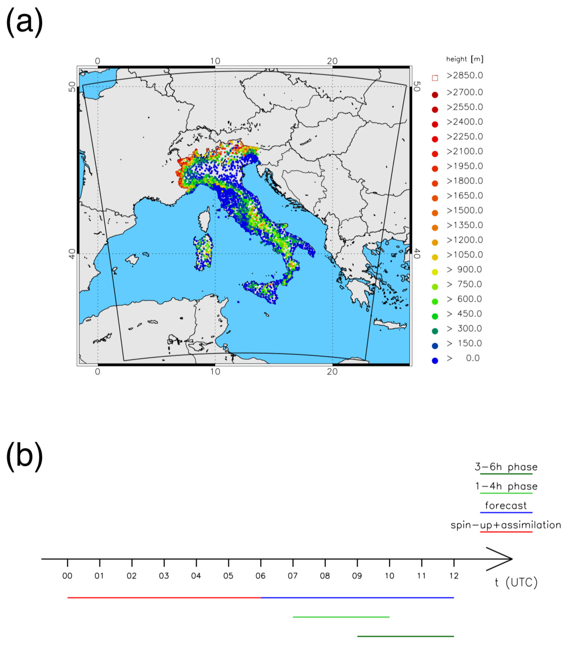
2.1. WRF Model Configuration and Experimental Set-Up

For the data assimilation experiments, we used the Weather Research and Forecasting model with advanced WRF dynamics (WRF-ARW) version 4.1.3 [23].
The main physical parameterisations considered for the WRF run are the following: The Thompson scheme [24] was employed as a microphysics scheme; the Mellor–Yamada–Janjic turbulence kinetic energy scheme [25] was used as the boundary layer scheme, and the Dudhia scheme [26] and rapid radiative transfer model (RRTM) [27] were applied as shortwave and longwave radiative schemes, respectively.
We considered one grid (Figure 1a), covering the Italian territory and parts of the Central Mediterranean and Central Europe, with 635 × 635 grid points in the N–S and W–E directions, a 3 km horizontal resolution, and 50 vertical levels, reaching the model’s top at 50 hPa.
The model was initialised using the 3-hourly operational analysis/forecast cycle at 0.25° from the European Centre for Medium-Range Weather Forecast’s (ECMWF’s) Integrated Forecast System (IFS), starting at 12 UTC on the day before the day to forecast.
The WRF model was run in four different configurations, depending on the assimilation application, the assimilated product, and the minimum threshold chosen for starting the assimilation (For a discussion on the choice of the thresholds, see Section 4.). The four configurations are summarised in Table 1.
For all four model configurations, we simulated 15 days for summer 2022 and 17 days for fall 2022. These two seasons are the most suitable for checking the capability of the rain rate assimilation to impact the precipitation forecast because of the predominant convective nature of their rainfall events [28]. Specifically, the year 2022 was characterised by several convective events in summer and fall. The days for the simulations were selected for events with observed moderate or intense precipitation (as registered by rain gauges), and the corresponding dates are reported in Table 2.
The simulations were performed following a very short-term forecast (VSF) approach (Figure 1b). In particular, each simulation was run in a 12 h period. The first 6 h are used as a spin-up time and for the assimilation of the NN_3th, NN_1th, and H60_3th rain rates, while the second 6 h are the forecast period. In the assimilation phase, one analysis per hour is produced, with a total of 7 analyses, i.e., the simulation starting time and the following 6 h. For each day, four different runs were executed, starting at 00, 06, 12, and 18 UTC. The model precipitation outputs are verified over the forecast period, considering two 3 h time intervals: the hours from 1 to 4 (1–4 h phase, i.e., times from 07 to 10 in Figure 1b, which is the sum of the precipitation recorded between 07 and 10) and the hours from 3 to 6 (3–6 h phase, i.e., times from 9 to 12 in Figure 1b, which is the sum of the precipitation recorded between 9 and 12) after the last assimilation time.
For the 1–4 h phase, verification starts from one hour after the end of the assimilation phase. In this way, the model output for the first of the three hours would be available for each run about half an hour before the occurrence of the real hour, making the results applicable in an ideal operational context. Supposing that rain rate products are available in near-real time (less than 20 min from the acquisition time) and considering the computational time needed for the last analysis and for the following 4 h run, it is reasonable to have the model output for the three hours composing the 1–4 h phase ready before the real occurrence of the 1–4 h phase. In other words, considering times as reported in Figure 1b, the prediction for the hour between time 07 and time 08 can be available at time 06:30, while the prediction for the three hours between time 07 and time 10 can be available before time 07. The 3–6 h phase is useful for studying the duration of the impact of the assimilation a few hours later. Even if there is a superimposition of one hour between the 1–4 h and 3–6 h phases, we choose to consider the results in periods with the same time length, i.e., in 3 h intervals, so that the results are directly comparable.

2.2. Rain Rate Products

We assimilated the rain rates estimated from two different products: a neural-network-based rain rate estimate (hereafter, NN) and the HSAF H60 product.
The H60 product is based on a blended rapid-update MW/IR technique (https://hsaf.meteoam.it/Products/ProductsList?type=precipitation, accessed on 13 May 2024; see also the H60 product user manual for details [29]; note that H60 was recently updated to H60B), where MSG SEVIRI IR images are combined with passive MW (PMW) precipitation estimates available from all the available PMW sensors (SSMIS, AMSU/MHS, AMSR-2, AMTS, and GMI). This product is provided at regular time intervals of 15 min in NRT (timeliness < 15 min), and its spatial coverage is the MSG full disc and includes Europe and the Mediterranean Basin, Africa, and the South Atlantic Ocean. The spatial resolution varies from 4.8 to 8 km, and the spatial sampling is consistent with the SEVIRI IR measurements (3 km at the nadir). Over the area considered in this study, the spatial resolution is about 5 km.
The artificial neural network’s rain rate is based on satellite measurements from the GPM constellation (global precipitation measurement) and MSG SEVIRI, adopting the methodology proposed by Sist et al. [30]. The data from the GPM constellation used in this work are provided by GMI, DPR, MHS, and SSMIS. This approach involves the implementation of two neural networks with an MLP (multilayer perceptron) architecture. The first (NN1) is designed to generate the rain mask, while the second (NN2) is responsible for estimating the precipitation rate. NN1 has as input the MSG SEVIRI cloud mask product [31] to obtain information on cloudy pixels within satellite imagery with high confidence (cloud mask product user guide [32]), and it is trained using the precipitation from the GPM (in millimetres per hour). The output of NN1 is the set of all the rainy pixels, which represent the input of NN2. NN2 is trained using the precipitation rate obtained from the GPM, and it produces the precipitation map used in the assimilation algorithm described below. According to Sist et al. [30] the two neural networks have different inputs from daytime and nighttime, but they have the same structure. In particular, all the NNs are based on MLP feedforward with 30 input neurons (or nodes), two hidden layers (with 80 nodes in the first and second layers for daytime and nighttime in NN1 and 100 nodes in the first and second layers for daytime and nighttime in NN2), and one output node. The activation functions for the hidden layers are a ReLU (rectified linear unit) and for the output, a sigmoid for NN1 and linear for NN2. The model has been trained using the samples indicated in Table 3, which refers to the dates used in [30], i.e., 5 June, 8 July, and 12 October 2015 and 20 February 2016. The training dataset was built using events from different days with respect to the day selected for the experiment, as indicated in Table 2; however, the WRF simulations using the ANN and those using H60 were conducted on the same days and verified against the same rain gauge data, making the comparison of the results fair. In addition, NNs and H60 use similar inputs (MSG IR and GPM PMW observations); however, they compute the rain rate in different ways, giving different estimations.
The final results, obtained with 1000 epochs, have an accuracy of 68.49% for NN1 nighttime and 87.03% for NN1 daytime. The MAE (mean absolute error) is 0.61 mm/h for NN2 nighttime and 0.78 mm/h for NN2 daytime. The final outputs of this NN approach consist of the rain rate (in millimetres per hour) for a given geographical area and a time interval. Its spatial and temporal resolutions depend on the MSG-SEVIRI product, e.g., 3 km at the sub-satellite point and 5 km at mid-latitudes, every 15 min. The outputs of the NNs were produced on demand for the cases reported in Table 2, but this methodology could be run in near-real time, similar to H60, with a time delay only due to the availability of the EUMETSAT data.

2.3. Rain Rate Data Assimilation Method

Rain rate data are assimilated through 3DVar. The 3DVar tool employed in this paper was developed at CNR-ISAC and was first used in combination with the RAMS@ISAC model [33] and then adapted to be used coupled with the WRF model. This 3DVar system has the capability to assimilate different kinds of observations: lightning data [34,35], radar reflectivity from ground-based radar [7,34] and from satellites [36], zenith total delay [37], and satellite-derived rain rate data [38].
In this paper, we use the following cloud model: We remap satellite rain rate estimations to a model grid, and we check the rain rate value at each grid point. For grid points where the estimated rain rate is above a certain threshold, we generate a relative humidity pseudo-profile, which is saturated along the atmospheric column in the layer between the LCL, estimated from the model output and the −25 °C isotherm (cloud top), and which has no data elsewhere. The minimum threshold used to activate the saturation is 3 mm/h for H60_3th and NN_3th or 1 mm/h for NN_1th. The choice of the threshold was made after conducting some experiments for each of the assimilated products, considering different thresholds. The best minimum threshold is a trade-off between correctly forecasting as many events as possible and limiting false alarms. A brief discussion about this choice will be reported later in this paper when discussing the results.
Because the parameter assimilated by the model is the water vapour mixing ratio, the relative humidity profiles are converted to the water vapour mixing ratio before applying 3DVar.
The 3DVar method consists of the minimisation of the cost function, given by
J x = 1 2 x x b T B 1 x x b + y O H x T R 1 [ y O H x ] ,
where x represents the state vector; x b is the background field; B and R are the background error matrix and the observation error matrix, respectively; y o   is the water vapour mixing ratio’s pseudo-profiles; and H is the observation operator, by which the water vapour mixing ratio’s profiles corresponding to the pseudo-observations are obtained. In the 3DVar formulation, the background error matrix (B) is decomposed in the three spatial directions: Bx, By, and Bz. The Bx and By matrices spread the analysis adjustment in the horizontal plane, applying a Gaussian decorrelation function, for which the length-scale depends on the level and is often computed with the NMC method [39]. In this paper, however, as we are assimilating water vapour corresponding to thunderstorms, the horizontal Gaussian length scale (the standard deviation of the Gaussian) is fixed at 15 km for all the levels in both the W–E and N–S directions. The observation error matrix is assumed to be diagonal. The water vapour mixing error decreases with height, starting from 3 g/kg at the surface; it is 1.0 g/kg at a 3 km height, 0.5 g/kg at a 5 km height, and 0.1 g/kg at a 7 km height. The vertical background error matrix takes into account the model error. The diagonal elements of Bz have twice the observation error at each level to give more weight to the observation than to the background in the analysis. Moreover, the error decorrelation length scale in the Bz matrix is 500 m, following the results of Federico et al. [34].
The cost function is minimised by means of the conjugate gradient method.

2.4. Verification Procedure

The precipitation forecast performances of the four different types of runs are calculated considering the comparison of the precipitation forecast with the rain gauge measurements of the Italian rain gauge network (Figure 1a). This network accounts for more than 4000 rain gauges over the Italian territory. Data are managed by regional administrations and are collected nationwide by the Italian Civil Protection Department [40]. The model forecast corresponding to a given rain gauge is computed as follows. We consider all the model grid points in a radius of 2 2 Δ x , where Δ x is the model grid spacing (3 km), and we select, among them, the grid point value in the best agreement with the observation.
Scores are computed based on a 2 × 2 contingency table (Table 4) for dichotomous events that can have only two values (“yes” or “no” in this case). For each threshold, the event is “the precipitation exceeds or is equal to the threshold”.
Considering the precipitation forecast and the corresponding rain gauge observation and a fixed rainfall threshold, a, b, c, and d in Table 4 have the following meanings:
-
hits (a): the precipitation forecast and rain gauge observation are both above or equal to the given threshold;
-
false alarms (b): the precipitation forecast is above or equal to the given threshold, while the rain gauge observation is below the given threshold;
-
misses (c): the precipitation forecast is below the given threshold, while the rain gauge observation is above or equal to the given threshold;
-
correct negatives (d): the precipitation forecast and observation are both below the given threshold.
The following precipitation scores are then calculated:
-
Frequency bias (FBIAS), which is a measure of the frequency of predicted events above a certain rainfall threshold with respect to the observed frequency.
F B I A S = a + b a + c
FBIAS varies between 0 and ∞, with the best value at 1;
-
Probability of detection (POD), which accounts for the number of correctly predicted events upon the number of observed events. The POD gives the capability to the model for forecasting the exceedance of a certain rainfall threshold in the domain. Values close to one indicate that the experiment has a near-perfect performance, while in contrast, values near zero show that the model cannot correctly forecast the events.
P O D = a a + c
-
Threat score (TS), which is the ratio between the number of events correctly predicted and the sum of the observed and predicted events.
T S = a a + b + c
-
False-alarm rate (FAR), which provides a measure of the fraction of rain forecast events that did not occur; therefore, a value of one signifies that only false alarms and no correct events were forecast; a value of zero denotes that only correct events and no false alarms were forecast.
F A R = b a + b
POD, TS, and FAR can assume values in the [0, 1] interval. POD and TS have 1 as the best value, while for the FAR, the best value is 0.
The above-mentioned scores are related each other and can be summarised through the widely used performance diagram [41]. The x-axis of this diagram is defined as the success ratio (SR = 1 − FAR); the y-axis is the POD; the straight lines from the origin represent FBIAS, and the hyperbolic branches are the TS. The upper-right corner corresponds to the perfect score.

3. Results

3.1. A Case Study

In this section, we show the impact of the rain rate data assimilation on the precipitation forecast for a case study. We focus on the 1–4 h phase after the assimilation, as it is the phase when the data assimilation impact is higher. The considered event occurred on 18 August 2022 in the time range between 07 and 10 UTC. Therefore, the simulation started at 00 UTC on the same day and assimilated rain rate data until 06 UTC. In Figure 2 and Figure 3, we show the rain rate estimates and the relative humidity innovations, i.e., the differences between the analyses and the background field, at the time of the last analysis assimilated in the WRF model (06 UTC). In Figure 2, we report the NN-derived rain rate estimate (Figure 2a) and the relative humidity innovation fields at a 2094 m height a.s.l. at 06 UTC for the NN_3th (Figure 2b) and for the NN_1th (Figure 2c) simulation types. Precipitation cells are mainly around Corsica Island, Northern Sardinia, and the surrounding sea, with rainfall swaths also over Liguria and Piedmont regions and on the Italian border with Austria and Switzerland. As a consequence of these signals, significant variations in relative humidity are found for NN_3th and NN_1th after the analysis. The higher-precipitation area, around Corsica Island, produced an increase in the relative humidity of more than 50% in both cases and over a more extended area for NN_1th. The H60 estimate (Figure 3a) also detects rainfall around Corsica and Northern Sardinia and over Liguria. Precipitation swaths over Northwestern Italy and over Northeastern Italy and Western Austria are shifted to the east compared to the NN product. The H60 rain rate values are higher compared to the NN estimate. The maxima reach more than 18 mm/h for H60 and less than 8 mm/h for the NN estimate. The H60_3th analysis produces relative humidity variations of 50–60% over the sea surrounding Corsica Island, covering a wider area compared to Figure 2b,c.
The impact of the rain rate assimilation on the precipitation forecast between 07 and 10 UTC on 18 August 2022 is shown in Figure 4.
Precipitation is located mainly over Liguria and Tuscany regions, as recorded by rain gauges (Figure 4a). The precipitation is, overall, moderate, with some intense peaks of more than 50 mm/3 h over Liguria. The control simulation (Figure 4c) predicts up to 40 mm/3 h over Liguria, but the simulated precipitation is about 80 km further west than the observed one, and the covered area is smaller than that in the observations. The H60_3th configuration (Figure 4d) predicts an intense event over Liguria, but precipitation maxima are not correctly located (The precipitation is shifted to the west compared to observations.), and the precipitation over the region is, overall, overestimated. False alarms over Piedmont are also produced, while precipitation over Tuscany is underestimated. In addition, intense precipitation is predicted over the sea, in front of Liguria. To test the model prediction also over the sea for this case study, we compare model outputs with the modified conditional merging (MCM) dataset.
MCM integrates precipitation measures coming from rain gauge measurements and radar estimates. The combination of these two sources of data is performed through a methodology called conditional merging [42]. Rain gauge data are available at different points in the domain, while radar data give information about the spatial structure of the precipitation field. These two kinds of data are merged, producing a gridded precipitation field. MCM data are available every half an hour, providing the precipitation accumulated over the last hour.
For this case study, MCM data (Figure 4b) report an intense precipitation event over the sea in front of the Liguria region and moderate precipitation between Sardinia and Tuscany. Therefore, the H60_3th prediction over the sea is partially reported by observations, but H60_3th produced a wider area of intense precipitation, resulting in a high rate of false alarms.
The simulation that assimilates the NN rain rate starting from a threshold of 3 mm/h (NN_3th) reproduces the event over the Liguria region, but the maxima are underestimated. Also, in this case, precipitation is apparent over the sea but at a lower extension and intensity compared to the H60_3th simulation. In this case, when compared with MCM, these prediction results underestimate the precipitation over the sea.
The simulation assimilating the NN-derived rain rate starting from a threshold of 1 mm/h (NN_1th) reproduces the precipitation over Liguria, better catching the location of the observed maxima. Even if two precipitation branches can be identified, different from observations, this is the only configuration that reproduces a part of the observed precipitation over Tuscany, predicting rainfall of up to 10–15 mm/3 h also for the southern part of the event. Nevertheless, the central part of the event in Tuscany remains underestimated also in this case. Furthermore, also for the NN_1th simulation, a high-precipitation event is predicted over the sea, in front of Liguria, which is more balanced than the other simulations with assimilation, because the area covered by intense precipitation is larger than that in the NN_3th simulation, in better agreement with MCM. Although some differences in the precipitation patterns can be identified also in this case, the precipitation maxima are better depicted, and at the same time, this simulation type does not reproduce a wide false-alarm area, as in H60_3th.

3.2. Scores for Summer and Fall

This section shows the statistical analyses of the precipitation predictions given by the four model configurations for summer and fall case studies. Two different periods are analysed, i.e., phases 1–4 h and 3–6 h, as described above. The results are shown through performance diagrams for three different precipitation thresholds, namely, 1 mm/3 h, 10 mm/3 h, and 30 mm/3 h.

3.2.1. Scores for the 1–4 h Phase

The results for the 1–4 h phase are reported in Figure 5. As regards the summer cases (Figure 5a), for the 1 mm/3 h threshold, all the simulations with rain rate assimilation have performances better than that of CTRL. The POD is about 70% for H60_3th and about 60% for NN_3th and NN_1th and about 50% for CTRL. Also, for the 10 mm/3 h thresholds, all the configurations with assimilation perform better than CTRL. The two configurations with the NN-derived rain rate show a lower POD (30%) than the configuration assimilating the H60 product (45%), but H60_3th also has a higher FAR compared to NN_3th and NN_1th. This difference in the FAR is more evident for the 30 mm/3 h threshold, where the H60_3th FAR is more than 70%, while NN_3th and NN_1th show a FAR of about 15% and 10%, respectively, showing the tendency of H60 to overestimate the rain rate. For this threshold, it is also noted that POD values are rather low compared to the other thresholds and are associated with low values of FBIAS, showing this model’s tendency to underestimate precipitation. However, an improvement with respect to the CTRL simulation is still gained when assimilation of the NN-derived product is performed.
Figure 5b shows the results for the case studies in fall. For all the thresholds, fall performances are better than summer ones (closer to the upper-right part of the diagram). For the 1 mm/3 h threshold, all the configurations perform in a similar manner. For the 10 mm/3 h threshold, a slight improvement is noted for simulations with assimilation compared to CTRL. As for the summer case studies, also for fall, for the highest threshold (30 mm/3 h), the H60_3th configuration shows a higher number of false alarms than the NN_3th and NN_1th simulation types, with similar values of POD for all the configurations. As a consequence of the increased FAR, H60_3th performs worse than CTRL for this threshold. Conversely, NN_3th and NN_1th improve the CTRL forecast.
In summary, in the hours from 1 to 4 after the assimilation, an improvement is obtained when assimilating rain rate data. This improvement is higher in summer than in fall. The model configuration assimilating the H60 product produces a higher number of false alarms than the assimilation of the neural-network-derived rain rate product. This increase in false alarms is coupled with a higher POD for the first two thresholds in summer but not in fall. When considering the highest threshold (30 mm/3 h) for both seasons, at an increase in false alarms, the H60_3th configuration does not correspond to an increase in POD, making H60_3th performances worse than that of CTRL for this threshold. Therefore, the overall performances are better for the two configurations assimilating the NN-derived rain rate data.

3.2.2. Scores for the 3–6 h Phase

It is interesting to study also the rain rate data assimilation effects on the precipitation forecast up to the sixth hour. For this purpose, we analyse, here, the second three hours after the assimilation. For summer (Figure 6a), the first two thresholds show better performances when assimilation is performed (for all the simulations), denoting the positive impact of the assimilation also for this time interval. For the higher threshold (30 mm/h), the performance behaviour is similar to that of the 1–4 h phase. In fact, also in this case, H60_3th has a high false-alarm rate (about 70%) compared to the values of 20–25% for NN_3th and NN_1th, with similar POD values, which, in any case, are lower compared to the other thresholds, denoting a decrease in the performances for more intense events.
For what concerns the fall statistics, all the simulations perform better than the summer simulations also in this forecast time interval. The performances of the four simulations are similar for the first two thresholds. An improvement with respect to CTRL is apparent for the highest threshold (30 mm/3 h) for the two NN_3th and NN_1th model configurations, while H60_3th performances are worse than those of CTRL.
All in all, we can summarise these results as follows: The positive impact of the rain rate data assimilation is still present for the 3–6 h phase for all the thresholds in summer and for the highest threshold in fall for the NN configuration. As for the 1–4 h phase, the highest threshold shows a higher number of false alarms for the H60_3th configuration, in particular, in summer, making simulations with neural-network-derived rain rates preferable.

4. Discussion

This paper has two objectives: to show that the satellite-derived rain rate data assimilation can improve the forecast of the rainfall in convective environments and to investigate if assimilating the rain rate estimate provided by the NN can improve the WRF precipitation forecast compared to the assimilation of the widely available in near-real-time H60 rain rate. The reason for choosing the H60 and NN rain rate products for the data assimilation is the following. H60 is an official rain rate product released by HSAF, satisfying the requirement of a suitable spatial–temporal resolution for data assimilation in rapid-update cycles. Moreover, H60 has a separate treatment for convective precipitation, taking into account the morphological information of clouds [29], making it a good candidate for data assimilation in convective environments. The NN used in this work is that of Sist et al. [30], which was shown to have good performances for the rain rate estimate starting from MSG-SEVIRI and other satellite observations. In addition, the NN can work in near-real time and satisfy the requirement of the high spatial–temporal resolution requested in a rapid-update cycle.
We considered a minimum threshold of 3 mm/h for the assimilation and two different precipitation products. For the NN product, the results of the assimilation for a minimum threshold of 1 mm/h are also shown. The forecast performance is evaluated over 15 case studies in summer 2022 and 17 case studies in fall 2022 for two forecast time intervals after the assimilation time: the hours from 1 to 4 (1–4 h phase) and the hours from 3 to 6 (3–6 h phase).
The choice of the minimum threshold employed to assimilate the rain rate can be explained as follows. As regards the neural-network-derived product, we first considered 3 mm/h as the minimum threshold for the assimilation, i.e., the NN_3th configuration shown in this paper. Because this configuration resulted in low PODs, especially when compared to the H60 assimilation for the highest precipitation threshold, we introduced a second experiment, NN_1th, allowing the model to saturate a higher number of grid cells. NN_1th gives slightly better POD values than NN_3th, without a significant increase in the FAR. The largest difference in the POD is observed in summer for the highest threshold, and NN_1th improves the performance of NN_3th. For the H60 product, we also started assimilating from the 3 mm/h threshold, i.e., the H60_3th configuration shown in this paper. For H60, however, the biggest issue was the high number of false alarms that were produced. Therefore, we ran the model with a second configuration, with a minimum threshold of 5 mm/h for the assimilation, adjusting the model over a lower number of grid cells compared to H60_3th. This second configuration is not shown in this paper because it did not give a noticeable improvement in the false alarms compared to the 3 mm/h threshold. Therefore, for the H60 product, we show only the results for the 3 mm/h threshold to make them directly comparable with the NN_3th model configuration. This result, however, suggests that higher thresholds could be explored in the future for H60, trying to improve the precipitation forecast assimilating the rain rate estimate of H60.
All the simulation experiments have been evaluated considering dichotomous statistical scores evaluated for three minimum thresholds of accumulated precipitation: 1 mm/3 h, 10 mm/3 h, and 30 mm/3 h.
In the 1–4 h phase, the rain rate assimilation improved the precipitation forecast with respect to the control simulation. The improvement is more significant in summer than in fall. The assimilation of the H60 product produced a higher FAR than the NN product and a higher POD but only for the first two thresholds in summer. For the 3–6 h phase, the rain rate data assimilation has a positive impact on the forecast for all the thresholds in summer and for the highest threshold in fall. Also, for this phase, the H60 product assimilation has a high number of false alarms, in particular, for summer and for the higher thresholds. This makes simulations with NN-derived rain rates preferable for both forecast phases and seasons.
The case study of 18 August 2022 shows a practical application of the rain rate assimilation. The most intense precipitation is mainly located over the Liguria region and over the sea in proximity to the Ligurian coast, as reported by rain gauges and by MCM. The simulations with assimilation reproduce the precipitation pattern over the Liguria region, not simulated by the control run, improving the forecast without rain rate data assimilation. In addition, these results show the better performance of the NN rain rate data assimilation compared to H60, mainly because the latter forecast has a higher number of false alarms.
The reasons for the high number of false alarms when the H60 product is assimilated compared to NNs are mainly three: (a) the higher rainfall rates estimated by H60; (b) the larger area covered by the precipitation estimated by H60; (c) the different positionings of rainfall spells in H60 and NN (the difference in the parallax correction). These characteristics of the rain rates estimated by H60 and NN were discussed in Section 3.1. Obviously, the first two characteristics cause an increase in the number of grid cells that are saturated in the WRF model when data assimilation is applied, and this causes the higher precipitation and false alarms when H60 is assimilated compared to NN. The third characteristic causes a shift in the rainfall pattens predicted by WRF using H60 or NN for data assimilation. This could also determine a higher number of false alarms when H60 is assimilated compared to NN. Quantifying the exact contribution of this point, however, is outside of the scope of this paper, where the focus is on evaluating the WRF forecast performance for two different satellite-derived rain rate products’ data assimilation.
Over Italy, there are not many works assimilating rain rates. The first attempt to assimilate rain rates was conducted in [17], with further application to hydrological forecasting in [18]. In these studies, however, the rain rate estimate was provided by rain gauge observations or by radar estimates and not by satellite. Recently, Gastaldo et al. [43] presented a study in which, among other experiments, the rain rate estimated using radar was assimilated in the Consortium for Small-Scale Modelling’s (COSMO’s) model. They showed that the rain rate assimilation can improve the COSMO rainfall forecast for up to 7 h (This time depends on the weather regime; see below.). However, in all these studies, the rainfall was assimilated from radar estimates or rain gauges, while in our work, we use satellite estimations. Of course, using satellite data has the advantage of data being available over the open sea, around Italy, as was shown for the 18 August 2022 case study, while radar and rain gauges are mainly available over the land. On the contrary, an issue of rain rates derived from satellites is the quality of the estimate, which can be lower compared to those derived from rain gauge or radar data sources.
An interesting aspect of our results is the larger improvement given by data assimilation in summer compared to fall. This behaviour is likely determined by the different weather regimes in these two seasons, which is related to the presence or absence of convective equilibrium. Craig et al. [44] suggested that the impact of the data assimilation is dependent on the weather regime and, in particular, the convective equilibrium/nonequilibrium [45]. When convection is in equilibrium with large-scale forcing, it consumes the instability that is generated by large-scale forcing. On the other hand, nonequilibrium convection (or triggered convection [46]) occurs when large-scale forcing is weak, and convection is triggered by local mechanisms that are able to overcome the convection inhibition. The latter convection regime is typical in summer, while the former regime is more typical in fall. Several studies [18,43,44,47] have shown that data assimilation has a higher impact on the nonequilibrium convective regime, and our study confirms those findings.
Overall, the results of this study show that satellite-derived rain rate data assimilation can improve the precipitation forecast of moderate to intense precipitation associated with convective events over the investigated study area. This improvement lasts until the sixth hour after the assimilation, suggesting the possibility, in an ideal operational context, to exploit this data assimilation set-up to take immediate actions when convective storms are approaching/developing. Artificial intelligence techniques can contribute to improve the model’s performance, and this study suggests that future developments in merging data assimilation and artificial intelligence techniques can have great potential for improving the forecast of localised convective precipitation events.

5. Conclusions

All in all, the results of this study can be pointed out as follows:
-
a method to assimilate satellite-derived rain rates into the WRF model is presented;
-
neural networks can estimate rain rates from satellite data;
-
neural-network-derived rain rate data assimilation can improve precipitation forecasts;
-
H60-derived rain rate data assimilation improves the forecast for the lower thresholds in summer, while producing a high number of false alarms for the highest threshold (30 mm/3 h).
Future works can aim at identifying storms’ convective cells, using artificial intelligence techniques, and focus on more complex rain rate assimilation, not by considering the minimum threshold for the assimilation but by considering actual precipitation rate values. The data assimilation of satellite measurements used for precipitation retrieval could be also taken into account in the future.

Author Contributions

Conceptualisation, R.C.T. and S.F.; methodology, R.C.T., M.P., F.D.F., S.D., G.P. and S.F.; software, R.C.T., M.P., A.M. and S.F.; validation, R.C.T. and M.P.; formal analysis, R.C.T.; investigation, S.F.; writing—original draft preparation, R.C.T., M.P., A.M., S.D., G.P. and S.F.; writing—review and editing, R.C.T., F.D.F., A.M., S.D., G.P. and S.F.; project administration, F.D.F. and S.F.; funding acquisition, F.D.F. and S.F. All authors have read and agreed to the published version of the manuscript.

Funding

This work was realised in the project AEROMET (AERO spatial data assimilation for METeorological weather prediction), funded by the Lazio Region—FESR Fondo Europeo di Sviluppo Regionale Programma Operativo regionale del Lazio, contract number A0375-2020-36588.

Data Availability Statement

H60 data are freely available at https://hsaf.meteoam.it. Neural network rainfall estimate can be requested to GEO-K (refer to M.P.). WRF simulations and the 3DVar software can be requested to the corresponding author. WRF simulations are available for 90 days after the publication of the paper.

Acknowledgments

The Italian Civil Protection Department is acknowledged for providing rain gauges and MCM data. Satellite rain-rate data for the H60 product are available through the HSAF website (https://hsaf.meteoam.it/, last accessed on 8 February 2024). Alessandra Mascitelli acknowledges financial support funded by the European Union Next-Generation EU, under the National Recovery and Resilience Plan (NRRP), mission 4 component 2-M4C2, investment 1.5 call for tender No. 3277 of 30 December 2021, Italian Ministry of University, award number: ECS00000041, project title: “Innovation, digitalisation, and sustainability for the diffused economy in Central Italy”, concession degree No. 1057 of 23 June 2022, adopted by the Italian Ministry of University, CUP: D73C22000840006.

Conflicts of Interest

The Author Mario Papa was employed by the GEO-K s.r.l. The remaining authors declare that the research was conducted in the absence of any commercial or financial relationships that could be construed as a potential conflict of interest. The funders had no role in the design of the study; in the collection, analyses, or interpretation of data; in the writing of the manuscript; or in the decision to publish the results.

References

  1. Clark, P.A.; Roberts, N.; Lean, H.W.; Ballard, S.P.; Charlton-Perez, C. Convection-permitting models: A step-change in rainfall forecasting. Meteor. Appl. 2016, 23, 165–181. [Google Scholar] [CrossRef]
  2. Cuo, L.; Pagano, T.C.; Wang, Q.J. A review of quantitative precipitation forecasts and their use in short- to medium-range streamflow forecasting. J. Hydrometeorol. 2011, 12, 713–728. [Google Scholar] [CrossRef]
  3. Stensrud, D.J.; Xue, M.; Wicker, L.J.; Kelleher, K.E.; Foster, M.P.; Schaefer, J.T.; Schneider, R.S.; Benjamin, S.G.; Weygandt, S.S.; Ferree, J.T.; et al. Convective-Scale Warn-on-Forecast System. Bull. Am. Meteorol. Soc. 2009, 90, 1487–1500. [Google Scholar] [CrossRef]
  4. Berner, J.; Fossell, K.R.; Ha, S.-Y.; Hacker, J.P.; Snyder, C. Increasing the skill of probabilistic forecasts: Understanding performance improvements from model-error representations. Mon. Weather Rev. 2015, 143, 1295–1320. [Google Scholar] [CrossRef]
  5. Dixon, M.; Li, Z.; Lean, H.W.; Roberts, N.M.; Ballard, S.P. Impact of data assimilation on forecasting convection over the United Kingdom using a high-resolution version of the Met Office Unified Model. Mon. Weather Rev. 2009, 137, 1562–1584. [Google Scholar] [CrossRef]
  6. Benjamin, S.G.; Weygandt, S.S.; Brown, J.M.; Hu, M.; Alexander, C.R.; Smirnova, T.G.; Olson, J.B.; James, E.P.; Dowell, D.C.; Grell, G.A.; et al. A North American hourly assimilation and model forecast cycle: The rapid refresh. Mon. Weather Rev. 2016, 144, 1669–1694. [Google Scholar] [CrossRef]
  7. Federico, S.; Torcasio, R.C.; Avolio, E.; Caumont, O.; Montopoli, M.; Baldini, L.; Vulpiani, G.; Dietrich, S. The impact of lightning and radar reflectivity factor data assimilation on the very short-term rainfall forecasts of RAMS@ISAC: Application to two case studies in Italy. Nat. Hazards Earth Syst. Sci. 2019, 19, 1839–1864. [Google Scholar] [CrossRef]
  8. Gustafsson, N.; Janjić, T.; Schraff, C.; Leuenberger, D.; Weissmann, M.; Reich, H.; Brousseau, P.; Montmerle, T.; Wattrelot, E.; Bučánek, A.; et al. Survey of data assimilation methods for convective-scale numerical weather prediction at operational centres. Q. J. R. Meteor. Soc. 2018, 144, 1218–1256. [Google Scholar] [CrossRef]
  9. Kidd, C.; Huffman, G. Global precipitation measurement. Meteor. Appl. 2011, 18, 334–353. [Google Scholar] [CrossRef]
  10. Krishnamurti, T.N.; Xue, J.; Bedi, H.S.; Ingles, K.; Oosterhof, D. Physical initialization for numerical weather prediction over the tropics. Tellus 1991, 43A, 53–81. [Google Scholar] [CrossRef]
  11. Krishnamurti, T.N.; Bedi, H.S.; Ingles, K. Physical initialization using SSM/I rain rates. Tellus 1993, 45A, 247–269. [Google Scholar] [CrossRef]
  12. Manobianco, J.; Koch, S.; Karyampudi, V.M.; Negri, A.J. The impact of assimilating satellite-derived precipitation rates on numerical simulations of the ERICA IOP 4 cyclone. Mon. Weather Rev. 1994, 122, 341–365. [Google Scholar] [CrossRef]
  13. Jones, C.D.; Macpherson, B. A latent heat nudging scheme for the assimilation of precipitation data into the mesoscale model. Meteor. Appl. 1997, 4, 269–277. [Google Scholar] [CrossRef]
  14. Stephan, K.; Klink, S.; Schraff, C. Assimilation of radar-derived rain rates into the convective-scale model COSMO-DE at DWD. Q. J. R. Meteor. Soc. 2008, 134, 1315–1326. [Google Scholar] [CrossRef]
  15. Falkovich, A.; Kalnay, E.; Lord, S.; Muthur, M.B. A new method of observed rainfall assimilation in forecast models. J. Appl. Meteor. 2000, 39, 1282–1298. [Google Scholar] [CrossRef]
  16. Sokol, Z. Effects of an assimilation of radar and satellite data on a very-short-range forecast of heavy convective rainfalls. Atmos. Res. 2009, 93, 188–206. [Google Scholar] [CrossRef]
  17. Davolio, S.; Buzzi, A. A Nudging Scheme for the Assimilation of Precipitation Data into a Mesoscale Model. Weather Forecast. 2004, 19, 855–871. [Google Scholar] [CrossRef]
  18. Davolio, S.; Silvestro, F.; Gastaldo, T. Impact of rainfall assimilation on high-resolution hydrometeorological forecasts over Liguria, Italy. J. Hydrometeorol. 2017, 18, 2659–2680. [Google Scholar] [CrossRef]
  19. Torcasio, R.C.; Federico, S.; Comellas Prat, A.; Panegrossi, G.; D’Adderio, L.P.; Dietrich, S. Impact of Lightning Data Assimilation on the Short-Term Precipitation Forecast over the Central Mediterranean Sea. Remote Sens. 2021, 13, 682. [Google Scholar] [CrossRef]
  20. Comellas Prat, A.; Federico, S.; Torcasio, R.C.; Fierro, A.O.; Dietrich, S. Lightning data assimilation in the WRF-ARW model for short-term rainfall forecasts of three severe storm cases in Italy. Atmos. Res. 2021, 247, 105246. [Google Scholar] [CrossRef]
  21. Janjić, T.; Bormann, N.; Bocquet, M.; Carton, J.A.; Cohn, S.E.; Dance, S.L.; Losa, S.N.; Nichols, N.K.; Potthast, R.; Waller, J.A.; et al. On the representation error in data assimilation. Q. J. R. Meteor. Soc. 2017, 144, 1257–1278. [Google Scholar] [CrossRef]
  22. Ebert, E.E. Fuzzy verification of high-resolution gridded forecasts: A review and proposed framework. Meteor. Appl. 2008, 15, 51–64. [Google Scholar] [CrossRef]
  23. Skamarock, W.C.; Klemp, J.B.; Dudhia, J.; Gill, D.O.; Liu, Z.; Berner, J.; Wang, W.; Powers, J.G.; Duda, M.G.; Barker, D.M.; et al. A Description of the Advanced Research WRF, Version 4; No. NCAR/TN-556+STR, NCAR Technical Note; National Center for Atmospheric Research: Boulder, CO, USA, 2019; 145p. [Google Scholar]
  24. Thompson, G.; Field, P.R.; Rasmussen, R.M.; Hall, W.D. Explicit Forecasts of Winter Precipitation Using an Improved Bulk Microphysics Scheme. Part II: Implementation of a New Snow Parameterization. Mon. Weather Rev. 2008, 136, 5095–5115. [Google Scholar] [CrossRef]
  25. Janjic, Z.I. The step-mountain eta coordinate model: Further developments of the convection, viscous sublayer, and turbulence closure schemes. Mon. Weather Rev. 1994, 122, 927–945. [Google Scholar] [CrossRef]
  26. Dudhia, J. Numerical study of convection observed during the Winter Monsoon Experiment using a mesoscale two-dimensional model. J. Atmos. Sci. 1989, 46, 3077–3107. [Google Scholar] [CrossRef]
  27. Mlawer, E.J.; Taubman, S.J.; Brown, P.D.; Iacono, M.J.; Clough, S.A. Radiative transfer for inhomogeneous atmospheres: RRTM, a validated correlated-k model for the longwave. J. Geophys. Res.-Space 1997, 102, 16663–16682. [Google Scholar] [CrossRef]
  28. Crespi, A.; Brunetti, M.; Lentini, G.; Maugeri, M. 1961–1990 high-resolution monthly precipitation climatologies for Italy. Int. J. Clim. 2018, 38, 878–895. [Google Scholar] [CrossRef]
  29. H60 Users Manual. Available online: https://hsaf.meteoam.it/CaseStudy/GetDocumentUserDocument?fileName=saf_hsaf_atbd_60-63_1_0.pdf&tipo=ATBD (accessed on 13 May 2024).
  30. Sist, M.; Schiavon, G.; Del Frate, F. A New Data Fusion Neural Network Scheme for Rainfall Retrieval Using Passive Microwave and Visible/Infrared Satellite Data. Appl. Sci. 2021, 11, 4686. [Google Scholar] [CrossRef]
  31. Derrien, M.; Le Gléau, H. MSG/SEVIRI cloud mask and type from SAFNWC. Int. J. Remote Sens. 2005, 26, 4707–4732. [Google Scholar] [CrossRef]
  32. EUMETSAT. Cloud Mask Product User Guide. Available online: https://navigator.eumetsat.int/product/EO:EUM:DAT:MSG:CLM (accessed on 28 March 2024).
  33. Federico, S. Implementation of a 3D-Var system for atmospheric profiling data assimilation into the RAMS model: Initial results. Atmos. Meas. Tech. 2013, 6, 3563–3576. [Google Scholar] [CrossRef]
  34. Federico, S.; Torcasio, R.C.; Puca, S.; Vulpiani, G.; Comellas Prat, A.; Dietrich, S.; Avolio, E. Impact of Radar Reflectivity and Lightning Data Assimilation on the Rain- fall Forecast and Predictability of a Summer Convective Thunderstorm in Southern Italy. Atmosphere 2021, 12, 958. [Google Scholar] [CrossRef]
  35. Torcasio, R.C.; Papa, M.; Del Frate, F.; Dietrich, S.; Toffah, F.E.; Federico, S. Study of the Intense Meteorological Event Occurred in September 2022 over the Marche Region with WRF Model: Impact of Lightning Data Assimilation on Rainfall and Lightning Prediction. Atmosphere 2023, 14, 1152. [Google Scholar] [CrossRef]
  36. Marra, A.C.; Federico, S.; Montopoli, M.; Avolio, E.; Baldini, L.; Casella, D.; D’Adderio, L.P.; Dietrich, S.; Sanò, P.; Torcasio, R.C.; et al. The Precipitation Structure of the Mediterranean Tropical-Like Cyclone Numa: Analysis of GPM Observations and Numerical Weather Prediction Model Simulations. Remote Sens. 2019, 11, 1690. [Google Scholar] [CrossRef]
  37. Mascitelli, A.; Federico, S.; Fortunato, M.; Avolio, E.; Torcasio, R.C.; Realini, E.; Mazzoni, A.; Transerici, C.; Crespi, M.; Dietrich, S. Data assimilation of GNSS-ZTD into the RAMS model through 3D-Var: Preliminary results at the regional scale. Meas. Sci. Technol. 2019, 30, 055801. [Google Scholar] [CrossRef]
  38. Federico, S.; Torcasio, R.C.; Mascitelli, A.; Del Frate, F.; Dietrich, S. Preliminary Results of the AEROMET Project on the Assimilation of the Rain-Rate from Satellite Observations. In Computational Science and Its Applications—ICCSA 2022 Workshops; Gervasi, O., Murgante, B., Misra, S., Rocha, A.M.A.C., Garau, C., Eds.; ICCSA 2022, Lecture Notes in Computer Science; Springer: Cham, Switzerland, 2022; Volume 13380, Available online: https://www.doi.org/10.1007/978-3-031-10542-5_36 (accessed on 13 May 2024).
  39. Parrish, D.F.; Derber, J.C. The National Meteorological Center’s Spectral Statis- tical Interpolation analysis system. Mon. Weather Rev. 1992, 120, 1747–1763. [Google Scholar] [CrossRef]
  40. Davolio, S.; Ferretti, R.; Baldini, L.; Casaioli, M.; Cimini, D.; Ferrario, M.E.; Gentile, S.; Loglisci, N.; Maiello, I.; Manzato, A.; et al. The role of the Italian scientific community in the first HyMeX SOP: An outstanding multidisciplinary experience. Meteorol. Z. 2015, 24, 261–267. [Google Scholar] [CrossRef]
  41. Roebber, P.J. Visualizing multiple measures of forecast quality. Weather Forecast. 2009, 24, 601–608. [Google Scholar] [CrossRef]
  42. Sinclair, S.; Pegram, G. Combining radar and rain gauge rainfall estimates using conditional merging. Atmosph. Sci. Lett. 2005, 6, 19–22. [Google Scholar] [CrossRef]
  43. Gastaldo, T.; Poli, V.; Marsigli, C.; Cesari, D.; Alberoni, P.P.; Paccagnella, T. Assimilation of radar reflectivity volumes in a pre-operational framework. Quart. J. Roy. Meteor. Soc. 2021, 147, 1031–1054. [Google Scholar] [CrossRef]
  44. Craig, G.C.; Keil, C.; Leuenberger, D. Constraints on the impact of radar rainfall data assimilation on forecasts of cumulus convection. Quart. J. Roy. Meteor. Soc. 2012, 138, 340–352. [Google Scholar] [CrossRef]
  45. Emanuel, K.A. Atmospheric Convection; Oxford University Press: Oxford, UK, 1994. [Google Scholar]
  46. Zimmer, M.; Craig, G.C.; Keil, C.; Wernli, H. 2011: Classification of precipitation events with a convective response timescale and their forecasting characteristics. Geophys. Res. Lett. 2011, 38, L05802. [Google Scholar] [CrossRef]
  47. Zeng, Y.; Janji’c, T.; Sommer, M.; de Lozar, A.; Blahak, U.; Seifert, A. Representation of model error in convective-scale data assimilation: Additive noise based on model truncation error. J. Adv. Model. Earth Syst. 2019, 11, 752–770. [Google Scholar] [CrossRef]
Figure 1. WRF model domain and rain gauge stations’ altitude (a); simulations’ scheme using the very short-term forecast approach (b).
Remotesensing 16 01769 g001
Figure 2. Rain rates estimated by the neural network (in millimetres per hour) (a), and the relative humidity innovation fields at 2094 m a.s.l. at 06 UTC on 18 August 2022 for the NN_3th (b) and the NN_1th (c) model configurations (in percentages).
Remotesensing 16 01769 g002
Figure 3. Rain rates estimated by H60 (a) and relative humidity field innovation (b) at 06 UTC on 18 August 2022 at 2094 m a.s.l. for the H60_3th configuration.
Remotesensing 16 01769 g003
Figure 4. Precipitation between 07 and 10 UTC on 18 August 2022, as reported by rain gauges (a) and MCM (b) and simulated by CTRL (c), H60_3th (d), NN_3th (e), and NN_1th (f) WRF model configurations.
Remotesensing 16 01769 g004
Figure 5. Performance diagrams for the CTRL, NN_3th, NN_1th, and H60_3th configurations and for the 1 mm/3 h, 10 mm/3 h, and 30 mm/3 h thresholds for the case studies in summer (a) and in fall (b) for the 1–4 h verification phase. Red hyperboles branches represent the threat score while cyan lines represent the frequency bias.
Remotesensing 16 01769 g005
Figure 6. Performance diagrams for the CTRL, NN_3th, NN_1th, and H60_3th configurations and for the 1 mm/3 h, 10 mm/3 h, and 30 mm/3 h thresholds for the case studies in summer (a) and in fall (b) for the 3–6 h verification phase. Red hyperboles branches represent the threat score while cyan lines represent the frequency bias.
Remotesensing 16 01769 g006
Table 1. Simulation types used in the numerical experiments.
Simulation TypeRain Rate
Assimilation
Assimilated ProductMinimum Threshold for the Assimilation
CTRLNoNoneNone
NN_3thYesRain rate derived from neural network3 mm/h
NN_1thYesRain rate derived from neural network1 mm/h
H60_3thYesRain rate derived from HSAF H60 product3 mm/h
Table 2. Days selected for the experiment.
Summer 2022
June7; 8; 9; 10; 17
July7; 8; 26; 27; 29
August9; 12; 17; 18; 19
Fall 2022
September15; 17; 22; 24; 25; 26; 29; 30
October10; 13
November4; 15; 16; 19; 22; 26; 29
Table 3. Samples used for NNs, depending on daytime and nighttime datasets.
NNTimeTotal
Samples
Training
Samples
Validation
Samples
Test
Samples
NN1day24,47117,12936713671
NN1night22,51215,75833773377
NN2day8516596012781278
NN2night7774544111671166
Table 4. Contingency table for dichotomous events.
Forecast
YesNo
ObservationYesac
Nobd
Disclaimer/Publisher’s Note: The statements, opinions and data contained in all publications are solely those of the individual author(s) and contributor(s) and not of MDPI and/or the editor(s). MDPI and/or the editor(s) disclaim responsibility for any injury to people or property resulting from any ideas, methods, instructions or products referred to in the content.

