
Analyzing the Effect of Tethered Cable on the Stability of Tethered UAVs Based on Lyapunov Exponents

1
School of Mechanical and Automobile Engineering, Shanghai University of Engineering Science, Shanghai 201600, China
2
Beijing Institute of Construction Mechanization Co., Ltd., Beijing 065000, China
*
Author to whom correspondence should be addressed.
Appl. Sci. 2024, 14(10), 4253; https://doi.org/10.3390/app14104253
Submission received: 9 April 2024
/
Revised: 12 May 2024
/
Accepted: 12 May 2024
/
Published: 17 May 2024
(This article belongs to the Special Issue Advanced Research and Application of Unmanned Aerial Vehicles)
Abstract
:In the working process of the tethered unmanned aerial vehicle (UAV), there is interference from the tethered cable, which can easily lead to the instability of the UAV. To solve the above problems, a method based on the Lyapunov exponent is proposed to analyze the stability of tethered cables for tethered UAVs. The dynamics equation of the UAV platform is established using the Euler–Poincare equation. The tension formula of the tethered cable is derived from the catenary theory and the principle of micro-segment equilibrium. Based on the Lyapunov exponential method, the stability changes of the tethered UAV in the takeoff, hovering, and landing stages are simulated and analyzed in a MATLAB environment. Prototype tests are carried out to prove the correctness of the simulation model and calculation conclusions. The results show that with an increase in the density of the tethered cable, the stability of the tethered UAV tends to decrease. At the same time, stability is affected by the density of the tethered cable more often during takeoff than during landing.
1. Introduction
As a new type of rotary-wing unmanned aerial vehicle (UAV), the tethered UAV comprises three parts: A ground power supply platform, a tethered cable, and a UAV platform. Tethered UAVs are widely used in scenarios such as personnel search and rescue [1,2], geological exploration [3,4], and fire monitoring [5] because of the advantages of long endurance, which is a trend in the future development of UAVs. However, tethered UAVs also have the problem of stability and susceptibility to interference. During the flight of the tethered UAV, there are factors such as gusts of wind interference, ground effect [6], aerodynamic effect [7,8], etc., that will cause the UAV to vibrate. At the same time, the uncontrolled instability caused by the above-influencing factors will continue to be amplified due to tethered cables. Tethered UAVs are expensive, and depending on the application, they can be equipped with expensive avionics such as searchlights, high-definition cameras, and high-performance sensors. To reduce the crash rate and improve the maneuverability of UAVs, it is necessary to study the influence of tethered cables on the motion stability of tethered UAVs.
There are generally two methods for studying the motion stability of UAVs. (1) Solving dynamic differential equations. This method has particular difficulties dealing with rotorcraft systems with high coupling, many variables, nonlinearity, and underdrive, so its versatility and popularization could be better. (2) Lyapunov function analysis. This method generally does not require the solution of cumbersome aerodynamic equations and is also quite popular for aircraft stability analysis [9]. There are two types of Lyapunov function analysis methods: Direct and exponential. For the direct method, Amiri et al. [10] obtained the dynamic model of the unconventional dual-fan UAV by the Newton–Euler method, analyzed its stability by Lyapunov’s direct method, and designed an integral backstepping control strategy to calm down the state quantities of the position and attitude loops on this basis. Islam et al. [11] studied a quadrotor’s nonlinear adaptive trajectory tracking problem under fault conditions based on the Lyapunov direct method. However, the Lyapunov direct method usually requires more work to construct a suitable function in the face of nonlinear and highly coupled systems. The ability to suppress external disturbances could be more vital, especially since giving quantitative system indicators is challenging. For the exponential method, the Lyapunov exponential method can quantitatively analyze the motion stability of the system and provide a precise evaluation index. Armiyoon et al. [12] evaluated the performance of the vehicle control system for yaw stabilization and rollover prevention by the Lyapunov exponent method. Liu et al. [13] established a quantitative relationship between structural parameters and the dynamic stability of a quadrotor UAV by employing the Lyapunov exponential method, which guided the optimization of the mechanical structure design of the vehicle and its stability control. Zhang et al. [14] investigated the quantitative relationship between the structural parameters of a quad-tilt wing-unmanned aerial vehicle and the dynamical stability of the system’s transition mode using the Lyapunov exponential method. Through the above literature research, it is found that some scholars’ research on aircraft stability mainly focuses on fixed-wing UAVs and quadrotor UAVs. There is no more in-depth analysis of tethered UAVs; stability studies do not explore the relationship with tethered cables.
Based on the above analysis, this paper uses a method based on the Lyapunov exponent to quantify the motion stability of tethered UAVs. The Euler–Poincare equation and catenary theory are used to obtain the dynamic equation of the tethered UAV. Then, based on the Lyapunov exponential method, the motion stability of the tethered UAV is analyzed in the simulation environment. The quantitative relationship between the tethered cable and the stability of the tethered UAV system is obtained. Finally, the prototype flight test is carried out to verify the simulation results.
2. Modeling of Tethered UAV Dynamics
Figure 1 shows the composition of the tethered UAV system, which mainly includes three parts: Ground power supply box, tethered cable, and UAV platform. The hardware composition of the tethered UAV is shown in Figure 2, which mainly includes the fuselage, power system, tethered system, sensor, control system, and power supply system. The difference between a tethered UAV and a normal rotary-wing UAV is the addition of a tethered cable. Therefore, when analyzing the tethered UAV system, it is usually divided into two parts: the UAV platform and the tethered cable.
2.1. Dynamics Modeling of UAV Platforms
2.1.1. Coordinate System Selection and Parameter Description
As shown in Figure 3, to describe the rotation and movement of an aerial UAV platform, it is necessary to use the airframe coordinate system OB-XB-YB-ZB. To determine the position of the UAV, it is essential to choose the ground coordinate system OE-XE-YE-ZE. In the body coordinate system, the linear displacement along the axial direction of OX, OY, and OZ is represented by x, y, and z, respectively, and the linear velocity is represented by u, v, and w, respectively. The attitude angles around the OX, OY, and OZ axes are defined by φ, θ, and ψ, respectively, and the angular velocities are expressed by p, q, and r, respectively. The moment of inertia around the OX, OY, and OZ axes is represented by Ix, Iy, and Iz, respectively, and Ixy, Iyz, and Ixz, respectively, define the inertia products of the XOY, YOZ, and XOZ planes. The lift and moment generated by the rotor of the UAV are expressed by Fi and Mi (i = 1,2,3,4), respectively.
2.1.2. Modeling Assumptions for UAV Platforms
The movement of the UAV is a very complex dynamic process, and its operating characteristics are affected by many factors. For example, the elasticity of the airframe, the change in weight acceleration with the altitude of flight, the Earth’s curvature, the speed of rotation, and the movement of the surrounding atmosphere. If all of these factors are included, the whole equation is complicated. It is not even possible to carry out the processing [15]. For simplicity, appropriate assumptions can be made when modeling the tethered UAV.
Hypothesis 1.
The UAV platform is a rigid body with invariant mass and moment of inertia. In this way, the elastic vibration and deformation of the UAV can be ignored, and the displacement, velocity, and acceleration of the rigid body can be analyzed directly to study the law of motion of the object.
Hypothesis 2.
The geometric center and center of gravity of the UAV platform and the origin of the fuselage coordinate system coincide. The geometry of the UAV is symmetrical with the internal mass distribution, that is, the inertia product Ixy = Iyx = 0.
Hypothesis 3.
Let the ground be an inertial frame of reference, ignore the effects of the earth’s curvature, rotation, and revolution, and treat the earth’s surface as a plane.
Hypothesis 4.
Acceleration due to gravity is constant. Since tethered UAVs usually fly at altitudes below 100 m, the change in gravitational acceleration due to the change in altitude can be ignored.
Hypothesis 5:
Wind resistance and gravity are not affected by flight altitude, and other external factors remain constant.
2.1.3. Force Analysis of the UAV Platform
When the UAV is working, the brushless motor usually rotates, driving the rotors to generate air flow to drive the UAV to complete various actions. There are three primary sources of force acting on a UAV. These include the vertical upward lift FT generated by the rotors, the gravity G, and the bollard pull T. Figure 4 is a schematic diagram of the force of the UAV platform.
In Figure 4, F1, F2, F3, and F4 are the lifts generated by the four rotors; M1, M2, M3, and M4 are the torques generated by each rotor; T is the tension of the tethered cable, and G is the gravity of the UAV platform. Since UAVs are mostly hovering when working in high-altitude environments, the angles of α and φ are approximately 0 degrees when analyzed. The amount of lift and torque is related to the speed of the rotor.
Changing the rotational speed of the rotor allows for different flight attitudes.
When F1 = F2 = F3 = F4, the UAV platform is in an ascending, descending, or hovering state;
When F2 = F4 and F1 ≠ F3, the system is in the pitch state;
When F1 = F3 and F2 ≠ F4, the system is in a roll state;
When F1 = F3 ≠ F2 = F4, the system is in yaw.
2.1.4. Dynamical Modeling
For dynamic modeling of UAV platforms, they are often thought of as rigid bodies. The UAV platform dynamics equation consists of a position and attitude dynamics equation. The traditional methods of attitude description are Euler angles, rotation matrices, quaternions, etc. Most of the dynamic modeling methods adopt traditional methods such as the Newton–Euler method [16], the Lagrange method [17], and the Kane method [18]. The dynamic model established by these methods has different expressions, but the final results of the dynamic characteristics of the described objects are the same. In this paper, the kinematics and dynamics equations of the UAV platform based on the Euler–Poincare equation are as follows [19]:
where p is the pseudo-velocity vector and q is the generalized coordinate vector. Their expressions are as follows:
V(q) kinematic transition matrix in the form of the following:
where represents the position transition matrix from the body coordinate system to the ground coordinate system and represents the attitude transition matrix from the body coordinate system to the ground coordinate system. The specific forms are:
where sφ is sinφ; sθ is sinθ; sψ is sinψ. The same goes for cos and tan.
M(q) is an inertia matrix of the form:
where m is the mass of the UAV platform.
C(q,p) is a gyroscopic matrix of the form:
F(p,q,u) is a fusion term containing aerodynamic forces, gravity, control inputs, and tether cable tension. Its specific form is as follows:
u = [U1, U2, U3, U4]T is the control input vector. The specific expression is:
where K = CQ/CT, CQ is the torque coefficient, and CT is the lift coefficient.
In addition, the lift and torque of the motor are calculated as follows [20]:
where ρa is the air density; A = πR2 is the rotating area of the paddle; R is the radius of the paddle; Ω is the rotational speed of the paddle.
2.2. Modeling of Tethered Cables
2.2.1. Modeling Assumptions for Tethered Cables
To model the tethered cable more accurately, the force of the cable needs to be analyzed. When the tethered UAV is in vertical lifting and lowering, the tethered cable only has a longitudinal force on the UAV platform. When the UAV platform moves horizontally, the tethered cable is in a state of traction, and the current force situation is complicated. Before proceeding with the force analysis, some assumptions about the tethered cable should be made to simplify the process and highlight the key points.
(1) The tether cable is assumed to be flexible. It can only withstand tensile forces but not pressures or bending moments [21]. Such an assumption is based on the physical properties of the cable material, which makes it possible to ignore the bending and compression deformation of the cable during force application during the analysis.
(2) It is assumed that the linear density of the tethered cable is constant. The material is uniformly distributed, and the cable is subjected only to self-weight loads that are uniformly distributed along the arc length. This means that the weight of the cable is uniformly distributed and does not change due to the change of position, which helps better calculate the forces on the cable in different states.
(3) It is assumed that the tethered cable’s elongation effect will not occur during the UAV’s movement. This assumption is based on the elastic properties of the cable material, which simplifies the deformation analysis of the cable when subjected to forces.
(4) Considering that the UAV mainly works in a breezy or windless environment, the disturbance effect of the lateral breeze is ignored here. This assumption helps to focus on the interaction between the tethered cable and the UAV rather than the impact of the external environment on the system.
2.2.2. Force Analysis of Tethered Cable
Under certain assumptions, tethered cables are mainly affected by two forces: I rope’s tension and gravity. In this paper, the force analysis of the tethered cable is carried out according to global mechanical equilibrium and micro-segment equilibrium principles and the related catenary theory [22]. The force analysis of the tether cable is shown in Figure 5.
Suppose the tensile force at one end of the tethered cable connected to the UAV platform is T1, and the angle between the tethered cable and the coordinate axis XE is α1. The tensile force at one end of the tethered cable connecting with the ground platform is T0, and the angle between the tethered cable and the coordinate axis XE is α0. According to the static analysis of the stress of the tethered cable, it can be seen that:
where the gravitational force of the tethered cable Gc = Lsε. LS is the length of the tethered cable. ε is related to the tethered cable material and represents the weight of the tethered cable per unit length.
2.2.3. Tension Formula
Assuming that the tethered cable extends 0 in the Y-axis direction, the cable satisfies the following geometric relation:
Dividing Equation (12) up and down yields the following:
From Equations (15) and (12), the following is derived:
Let T0cosα0 = H, then Equation (16) can be transformed into:
Taking the angle between the boundary condition tether cable and the X-axis to be 0, it can be obtained:
The tension equation for the tethered cable is then obtained as follows:
H and the maximum cable tension T can be found in (18) and (19).
When the tethered UAV performs various movements in the air, its force state will constantly change. As the UAV continues to rise, the gravity of the cable itself will increase accordingly. During horizontal movement, the expansion and contraction of the cable will also be affected, further changing the force situation of the UAV. To cope with these complex force variations, we assume that there is a maximum tensile force T, which represents the limit value of the cable when subjected to tensile forces. The tether cable’s tension T on the UAV platform is decomposed in ground coordinates to obtain the components Tx, Ty, and Tz of T in the X, Y, and Z axes, respectively, viz:
Further, generalizing the tether cable tension into a column vector of R6×1, there is:
2.3. DynamiIing of Tethered UAVs
The dynamic model of the tethered UAV can be obtained from the dynamic equations of the UAV platform in Section 2.1, plus the tension of the tethered cable in Section 2.2. Substitute Equation (21) into Equation (1) to solve the dynamics model. The first-order derivatives of the system state quantities p and q are obtained as:
Finally, Equations (22) and (23) are transformed into equations of state of the system. The complete dynamics model of a tethered UAV is described in the form of state space:
where X = [q, p]T = [x y z φ θ ψ u v w p q r].
3. Stability Analysis Based on Lyapunov Exponential Method
3.1. Lyapunov Exponent Calculation Process
The Lyapunov exponent is an important quantitative indicator for measuring the dynamics of a system. It characterizes the average exponential rate of convergence or divergence between adjacent orbits in phase space. There are generally two ways to calculate the Lyapunov exponent: One is based on a dynamical model, and the other is based on time series. Due to the time delay, time interval, evolution time and embedding dimension of the time series are difficult to determine. Therefore, this paper calculates the Lyapunov exponent based on the dynamics model. It is calculated as follows:
The equation of state is obtained by transforming the dynamical equation of a nonlinear system. The magnitude of the Lyapunov exponent λ is determined by the Jacobian matrix |df(X)\/dX|, where the function f(X) is at Xi. The formula for calculating the Jacobian matrix is as follows:
where denotes the eIement Xi (i = 1, 2, …, 12) in row i, column 1 of the derivative of the system state equation denotes the elemenI Xi in row i, column 1 of the system state equation X = [q, p]T. This section may be divided by subheadings. It should provide a concise and precise description of the experimental results, their interpretation, and the experimental conclusions that can be drawn.
Based on the established dynamics model, the Lyapunov exponential spectrum can be calculated by bringing Equation (24) into Equation (25). The specific flow of tethered machine motion stability analysis based on the Lyapunov exponent is shown in Figure 6. Among them, the number of iterations is 100, the step size is 0.5, the sampling time is 100 s, and the initial values of the system state quantities are all zero.
3.2. Parameterization of Dynamical Models
In the simulation experiment, the dynamic equation of the tethered UAV is first wrIin the MATLAB environment. After obtaining the equation, the flight conditions under different flight stages are obtained through the flight principle of the tethered UAV, and the corresponding Lyapunov exponential spectrum is simulated in MATLAB R2016b. The analysis shows that to establish a dynamic model of the quadrotor, it is necessary to obtain the following parameters: m, g, L, CT, CQ, R, K, Ix, Iy, Iz. A tethered UAV test prototype platform is built to obtain the above parameters, which mainly included three parts: the UAV platform, tethered cable, and ground power supply box, as shown in Figure 7.
The parameters of the tethered UAV platform can be determined by either a direct or indirect measurement method. Among them, the weight of the UAV platform m = 1.365 kg, the arm length L = 0.225 m, and the blade radius R = 0.127 m that can be directly measured. The local gravitational acceleration g = 0.98 m/s2 can be obtained by looking up the local reference book. Air density ρa = 1.293 kg/m3. The moment of inertia Ix and Iy can be measured indirectly by the two-wire suspension method, and the moment of inertia Iz can be measured by the four-wire suspension method. The lift coefficient CT and the reaction torque coefficient of the motor tensile experiment can be used to measure CQ. Finally, the tethered UAV’s structural parameters are shown in Table 1.
3.3. MATLAB Simulation Analysis
The above parameters of the tethered UAV are substituted into the dynamic equation of the tethered UAV for simulation analysis. Set the simulation type, simulation time, simulation step size, etc., and start the simulation after completing the simulation settings. After the simulation, the change of the Lyapunov exponent of the tethered UAV system with the density parameter of the tethered UAV system can be obtained using the post-processing tool. According to the actual flight conditions of the tethered UAV, the simulation is divided into takeoff, hovering, and landing.
3.3.1. Takeoff Stage
When the tethered UAV is in the takeoff phase, the Liapunov exponential spectrum of the tethered UAV can be obtained by simply varying the density ρ of the tether cable, as shown in Figure 8.
Further, the results of Figure 8 are statistically analyzed. The results of the numerical quantitative analysis of the Lyapunov exponential spectrum are shown in Table 2, where the data in parentheses represent the percentage change in the Lyapunov exponent. (↑: Indicates the percentage increase in the Lyapunov index; ↓: Indicates percentage decrease in the Lyapunov index; ─: Indicates that the Lyapunov Index remains unchanged).
As can be seen from Table 2, λ(φ), λ(θ) and λ(ψ) do not change much. When the density of the tethered cable is changed from ρ = 0.92 g/cm3 to ρ = 1.38 g/cm3, λ(φ), λ(θ), and λ(ψ) increase by 10.56%, 9.84%, and 13.14%, respectively. When the density of the tethered cable changes from ρ = 0.92 g/cm3 to ρ = 1.84 g/cm3, λ(x), λ(y), and λ(z) increase by 19.9%, 18.58%, and 24.45%, respectively. It can be seen that as the density of the tethered cable increases by 50% and 100% from 0.92 g/cm3 to 1.38 g/cm3 and 1.84 g/cm3, the Lyapunov exponent of the tethered UAV increases in a near-equivalent scale. Based on the definition of the Lyapunov exponent, it can be seen that the stability of the tethered UAV decreases as the density of the tether cable increases. Assuming that the overall stability can be described using the sum of the percent change amplitude of all channel state quantities, the overall stability of the tethered UAV decreases by 32.47% when the tethered cable density changes from ρ = 0.92 g/cm3 to ρ = 1.38 g/cm3. When the tether cable density changes from ρ = 0.92 g/cm3 to ρ = 1.84 g/cm3, the overall stability of the tethered UAV decreases by 61.07%.
3.3.2. Hovering Stage
When the tethered UAV is in the hovering phase, the Liapunov exponential spectrum variation of the tethered UAV can be obtained by simply varying the tether cable density ρ, as shown in Figure 9.
Further, the results of Figure 9 are statistically analyzed, and the numerical quantification of the Lyapunov exponential spectrum is shown in Table 3.
As seen from Table 3, since the change in the final value of the Lyapunov exponent is considered, the Lyapunov exponent of the tethered UAV does not change much during the hovering phase. Therefore, the change in state quantities in the hovering phase is similar to the takeoff phase. The overall stability of the tethered UAV decreased by 32.49% under tethered cable density ρ = 1.38 g/cm3 than ρ = 0.92 g/cm3. The overall stability of the tethered UAV decreased by 61.12% in the condition of tether cable density ρ = 1.84 g/cm3 over ρ = 0.92 g/cm3.
3.3.3. Landing Stage
When the tethered UAV is in the landing phase, the Liapunov exponential spectrum of the tethered UAV can be obtained by simply varying the tether cable density ρ, as shown in Figure 10.
Further, the results of Figure 10 are statistically analyzed, and the numerical quantification of the Lyapunov exponential spectrum is shown in Table 4.
From Table 4, it can be seen that in the landing stage, when the tethered cable density changes from ρ = 0.92 g/cm3 to ρ = 1.38 g/cm3, λ(x) and λ(y) increase by 5.75% and 6.77%, respectively. When the tethered cable density is changed from ρ = 0.92 g/cm3 to ρ = 1.84 g/cm3, λ(x) and λ(y) rise by 10.96% and 12.76%, respectively. λ(z), λ(φ), λ(θ), and λ(ψ) do not change much with the change in tethered cable density. Assuming that the overall stability can be described using the sum of the percent change amplitude of all channel state quantities, the overall strength of the tethered UAV decreases by 14.63% when the tether cable density is changed from ρ = 0.92 g/cm3 to ρ = 1.38 g/cm3. The overall stability of the tethered UAV decreased by 24.75% when the density of the tethered cable was changed from ρ = 0.92 g/cm3 to ρ = 1.84 g/cm3. The stability of the tethered UAV in the landing phase changed less with the tether cable density than in the takeoff phase.
4. Flight Tests
A prototype platform is built to conduct the external field test to verify the simulation model’s feasibility and the calculations’ accuracy. The prototype platform is shown in Figure 7. Specifically, the tethered UAV platform is selected to have a frame wheelbase of L = 450 mm and a blade of JMRRC 8045. By replacing different materials, the tethered cable is chosen to have a density of ρ = 0.92 g/cm3 and ρ = 1.38 g/cm3 for the comparative test. It should be added here that the flight control system of the test prototype built in this paper adopts APM2.8, and the ground control station is Missionplanner. The MP ground station operation interface and the flight log are shown in Figure 11. After the MissionPlanner ground station has planned the flight mode and trajectory of the tethered UAV, the tethered cables of different densities are replaced to carry out the autonomous mission. The tethered UAV carries out the mission autonomously, as shown in Figure 12, and the tethered UAV goes through the three phases of takeoff, hovering, and landing.
The flight log data in the flight control are shown in Figure 13 and Figure 14. The flight log data are processed, and the results are shown in Figure 15. Analyzing Figure 15, it can be learned that when the density of the tether cable is ρ = 0.92 g/cm3, the position change of the tethered UAV in the x and y directions is smaller than that when ρ = 1.38 g/cm3, which can be used to validate the results in Figure 8 as well as Table 2. This proves that the simulation model built in this experiment and the prototype model are correct. It also proves that increasing the tether cable’s density will harm the tethered UAV’s stability.
5. Conclusions
In this paper, the tethered cable’s influence on the UAV’s stability is studied for the complete flight process (takeoff–hover–landing) of the tethered UAV. This paper proposed a system stability analysis method based on the Lyapunov exponent. The dynamic model of the tethered UAV is obtained based on the Euler–Poincare equation and catenary theory. Converted to a MATLAB program to calculate the Lyapunov exponential spectrum. The effect of tether cable on the stability of the tethered UAV is obtained by changing the density of the tether cable. At the same time, flight tests are conducted based on the built F450 tethered UAV prototype. On this basis, the test is conducted by replacing the tether cable with different materials. The results show that:
(1) The overall stability of the tethered UAV during the takeoff phase is lower than during the landing phase, and the stability of the takeoff phase is more affected by the density of the tether cable.
(2) The system’s stability decreases with the increase in the tethered cable’s density. In the takeoff stage, with the rise in density by 50% and 100%, the stability decreased by 32.47% and 61.07%, respectively. The hovering stage is similar to the takeoff stage. In the landing stage, with the increase in density by 50% and 100%, the stability decreased by 14.63% and 24.75%, respectively.
(3) In the hovering stage, the stability of the tethered UAV is the best, and the UAV does not fluctuate greatly.
(4) The comparison of the prototype test results and the simulation results shows that the simulation model established in this paper is feasible.
Author Contributions
All authors contributed to the study’s conception and design. Material preparation, data collection, and analysis were performed by Z.T., C.L., H.J., F.H. and S.W. The first draft of the manuscript was written by Z.T. and C.L. and all authors commented on previous versions of the manuscript. All authors have read and agreed to the published version of the manuscript.
Funding
This research received no external funding.
Data Availability Statement
The raw data supporting the conclusions of this article will be made available by first author on request.
Conflicts of Interest
Author Shenglan Wang was employed by the company Beijing Institute of Construction Mechanization Co., Ltd. The remaining authors declare that the re-search was conducted in the absence of any commercial or financial relationships that could be construed as a potential conflict of interest.
References
- Radiansyah, S.; Kusrini, M.D.; Prasetyo, L.B. Quadcopter applications for wildlife monitoring. IOP Conf. Ser. Earth Environ. Sci. 2017, 54, 012066. [Google Scholar] [CrossRef]
- Senthilnath, J.; Kandukuri, M.; Dokania, A.; Ramesh, K.N. Application of UAV imaging platform for vegetation analysis based on spectral-spatial methods. Comput. Electron. Agric. 2017, 140, 8–24. [Google Scholar] [CrossRef]
- Fraundorfer, F.; Heng, L.; Honegger, D.; Lee, G.H.; Meier, L.; Tanskanen, P.; Pollefeys, M. Vision-based autonomous mapping and exploration using a quadrotor MAV. In Proceedings of the 2012 IEEE/RSJ International Conference on Intelligent Robots and Systems 2012, Algarve, Portugal, 7–12 October 2012; pp. 4557–4564. [Google Scholar]
- Faessler, M.; Fontana, F.; Forster, C.; Mueggler, E.; Pizzoli, M.; Scaramuzza, D. Autonomous, vision-based flight and live dense 3D mapping with a quadrotor micro aerial vehicle. J. Field Robot. 2016, 33, 431–450. [Google Scholar] [CrossRef]
- Moran, C.J.; Seielstad, C.A.; Cunningham, M.R.; Hoff, V.; Parsons, R.A.; Queen, L.; Sauerbrey, K.; Wallace, T. Deriving Fire Behavior Metrics from UAS Imagery. Fire 2019, 2, 36. [Google Scholar] [CrossRef]
- Anh, T.H.; Binh, N.T.; Song, J.W. In-Ground-Effect Model Based Adaptive Altitude Control of Rotorcraft Unmanned Aerial Vehicles. IEEE Robot. Autom. Lett. 2021, 7, 794–801. [Google Scholar] [CrossRef]
- Viegas, C.; Chehreh, B.; Andrade, J.; Lourenço, J. Tethered UAV with Combined Multi-rotor and Water Jet Propulsion for Forest Fire Fighting. J. Intell. Robot. Syst. 2022, 104, 20–21. [Google Scholar] [CrossRef]
- Chen, R.; Yuan, Y.; Thomson, D. A review of mathematical modelling techniques for advanced rotorcraft configurations. Prog. Aerosp. Sci. 2021, 120, 100681. [Google Scholar] [CrossRef]
- Abdelmaksoud, S.I.; Mailah, M.; Abdallah, A.M. Control Strategies and Novel Techniques for Autonomous Rotorcraft Unmanned Aerial Vehicles: A Review. IEEE Access 2020, 8, 195142–195169. [Google Scholar] [CrossRef]
- Amiri, N.; Ramirez-Serrano, A.; Davies, R.J. Integral Backstepping Control of an Unconventional Dual-Fan Unmanned Aerial Vehicle. J. Intell. Robot. Syst. 2013, 69, 147–159. [Google Scholar] [CrossRef]
- Islam, S.; Liu, P.X.; El Saddik, A. Nonlinear adaptive control for quadrotor flying vehicle. Nonlinear Dyn. 2014, 78, 117–133. [Google Scholar] [CrossRef]
- Armiyoon, A.R.; Wu, C.Q. Lyapunov exponents-based stability analysis and integrated control of rollover mitigation and yaw stabilisation of ground vehicles. Int. J. Veh. Syst. Model. Test. 2016, 11, 343–362. [Google Scholar] [CrossRef]
- Liu, Y.; Chen, C.; Wu, H.; Zhang, Y.; Mei, P. Structural stability analysis and optimization of the quadrotor unmanned aerial vehicles via the concept of Lyapunov exponents. Int. J. Adv. Manuf. Technol. 2018, 94, 3217–3227. [Google Scholar] [CrossRef]
- Zhang, Y.; Deng, Y.; Liu, Y.; Wang, L. Dynamics Modeling and Stability Analysis of Tilt Wing Unmanned Aerial Vehicle during Transition. Comput. Mater. Contin. 2019, 59, 833–851. [Google Scholar] [CrossRef]
- Liu, Y.; Li, X.; Wang, T.; Zhang, Y.; Mei, P. Quantitative stability of quadrotor unmanned aerial vehicles. Nonlinear Dyn. 2017, 87, 1819–1833. [Google Scholar] [CrossRef]
- Papachristos, C.; Alexis, K.; Tzes, A. Hybrid model predictive flight mode conversion control of unmanned quad-tiltrotors. In Proceedings of the 2013 European Control Conference (ECC) 2013, Zurich, Switzerland, 17–19 July 2013; pp. 1793–1798. [Google Scholar]
- Jain, A.; Rodriguez, G. Diagonalized Lagrangian robot dynamics. IEEE Trans. Robot. Autom. 1995, 11, 571–584. [Google Scholar] [CrossRef]
- Cheng, G.; Shan, X. Dynamics analysis of a parallel hip joint simulator with four degree of freedoms (3R1T). Nonlinear Dyn. 2012, 70, 2475–2486. [Google Scholar] [CrossRef]
- García Carrillo, L.R.; Dzul López, A.E.; Lozano, R.; Pégard, C.; García Carrillo, L.R.; Dzul López, A.E.; Pégard, C. Vision-based control of a quad-rotor uav. In Quad Rotorcraft Control: Vision-Based Hovering and Navigation; Springer: Berlin/Heidelberg, Germany, 2013; pp. 103–137. [Google Scholar]
- Chen, L.; Xiao, J.; Zheng, Y.; Alagappan, N.A.; Feroskhan, M. Design, Modeling, and Control of a Coaxial Drone. IEEE Trans. Robot. 2024, 40, 1650–1663. [Google Scholar] [CrossRef]
- Tao, Y.; Zhang, S. Research on the Vibration and Wave Propagation in Ship-Borne Tethered UAV Using Stress Wave Method. Drones 2022, 6, 349. [Google Scholar] [CrossRef]
- Qin, J.; Peng, F.; Qiao, L.; Jiang, M. Catenary method of helicopter live-line work in transmission line. In Proceedings of the 2016 International Conference on Advanced Electronic Science and Technology (AEST 2016) 2016, Shenzhen, China, 19–21 August 2016; pp. 969–974. [Google Scholar]
Figure 1.
System components of a tethered UAV.

Figure 2.
Hardware components of a tethered UAV.

Figure 3.
Coordinate system of the UAV platform.

Figure 4.
Force analysis of the UAV platform.

Figure 5.
Force analysis of tethered cable.

Figure 6.
Flow of Lyapunov exponent calculation.

Figure 7.
Physical drawing of the tethered UAV prototype.

Figure 8.
Lyapumov exponential spectra at different cable densities during the takeoff stage.

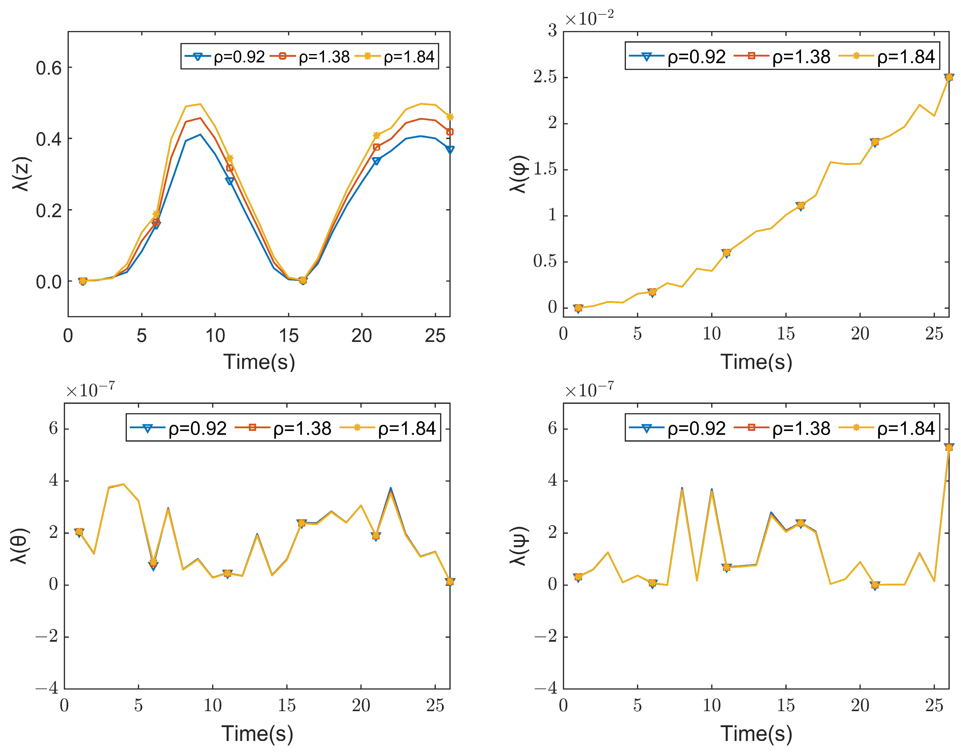
Figure 9.
Lyapunov exponential spectra for different cable densities during the hovering stage.

Figure 10.
Lyapunov exponential spectra for different cable densities during the landing stage.
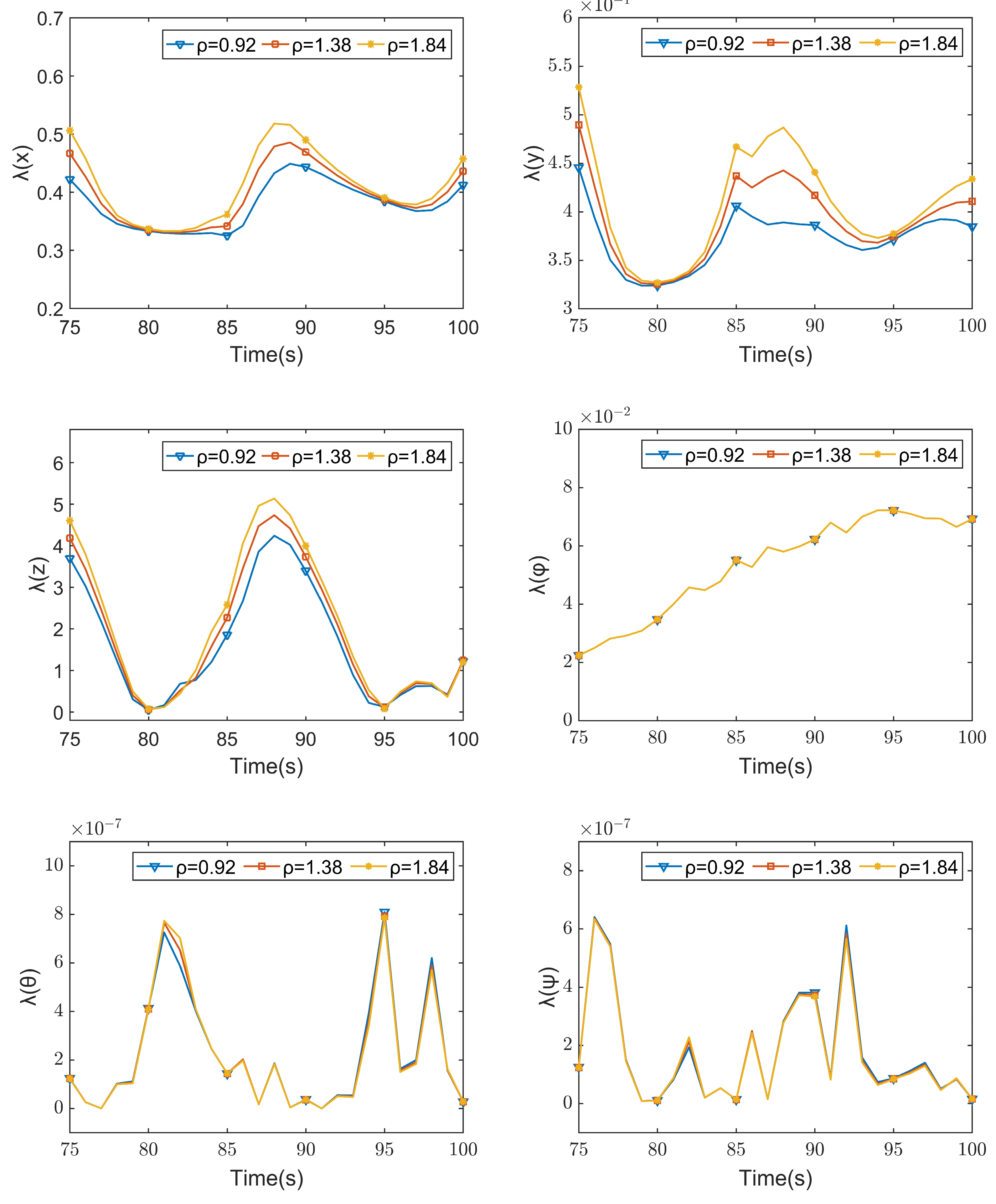
Figure 11.
MissionPlanner ground station interface and flight log interface.

Figure 12.
Real-life flight test of a tethered UAV.
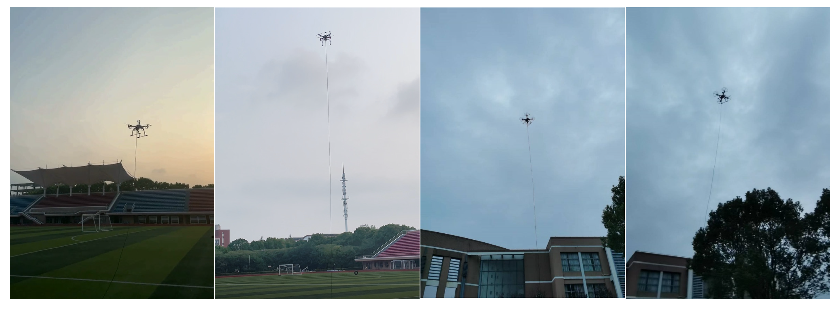
Figure 13.
Displacement in x-direction during flight: (a) ρ = 0.92, (b) ρ = 1.38.
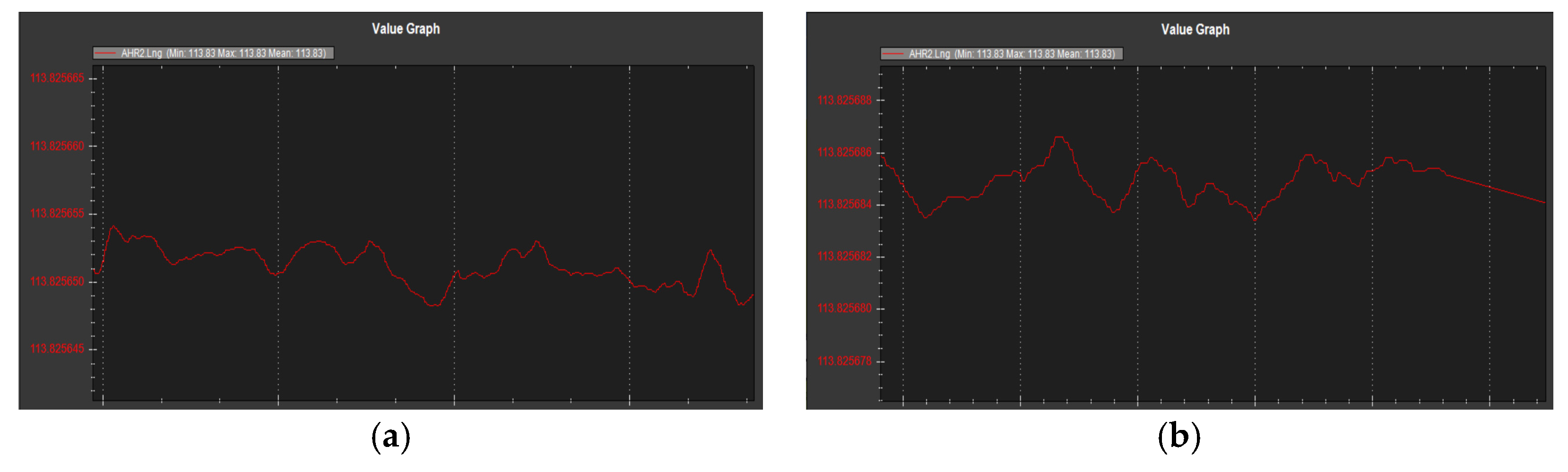
Figure 14.
Displacement in y-direction during flight: (a) ρ = 0.92, (b) ρ = 1.38.
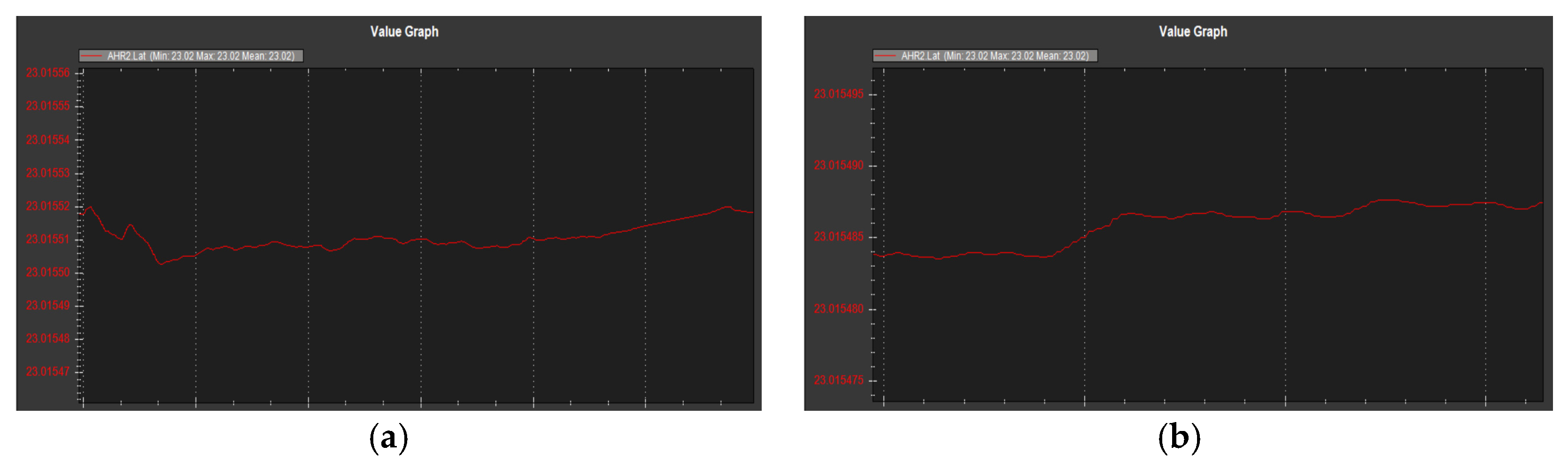
Figure 15.
Displacement in x- and y-directions during takeoff.


Table 1.
Physical parameters of tethered UAVs.
| Parameter | Meaning | Parameter Value |
|---|---|---|
| m | UAV platform weight | 1.365 kg |
| g | Gravity acceleration | 9.8 m/s2 |
| L | Boom length | 0.225 m |
| CT | Lift coefficient | 1.0792 × 10⁻⁵ |
| CQ | Reverse moment coefficient | 1.8992 × 10⁻⁵ |
| R | Blade radius | 0.127 m |
| Ix | Moment of inertia around the x-axis | 0.2868 kg/m2 |
| Iy | Moment of inertia around the y-axis | 0.3141 kg/m2 |
| Iz | Moment of inertia around the z-axis | 0.147 kg/m2 |
| ρa | Air density | 1.293 kg/m3 |
| ρ | Density of tethered cable | 1.29 kg/m3 |
| s | Cross-sectional area of a tethered cable | 0.002 m2 |
Table 2.
Final values of Lyapunov exponent at different cable densities during the takeoff stage.
| Parameter | ρ = 0.92 | ρ = 1.38 | ρ = 1.84 |
|---|---|---|---|
| λ(x) | 0.42195 | 0.46652 (↑ 10.56%) | 0.50592 (↑ 19.9%) |
| λ(y) | 0.44627 | 0.49017 (↑ 9.84%) | 0.52917 (↑ 18.58%) |
| λ(z) | 0.36989 | 0.41851 (↑ 13.14%) | 0.46032 (↑ 24.45%) |
| λ(φ) | 0.02505 | 0.02505 (─) | 0.02505 (─) |
| λ(θ) | 1.39 × 10⁻⁸ | 1.38 × 10⁻⁸ (↑ 0.53%) | 1.38 × 10⁻⁸ (↓ 0.92%) |
| λ(ψ) | 5.33 × 10⁻⁷ | 5.30 × 10⁻⁷ (↑ 0.54%) | 5.28 × 10⁻⁷ (↓ 0.93%) |
Table 3.
Final values of Lyapunov exponent for different cable densities during the hovering stage.
| Parameter | ρ = 0.92 | ρ = 1.38 | ρ = 1.84 |
|---|---|---|---|
| λ(x) | 0.42187 | 0.46646 (↑ 10.57%) | 0.50588 (↑ 19.91%) |
| λ(y) | 0.44572 | 0.48955 (↑ 9.83%) | 0.52851 (↑ 18.58%) |
| λ(z) | 0.36967 | 0.41835 (↑ 13.17%) | 0.46020 (↑ 24.49%) |
| λ(φ) | 0.02244 | 0.02244 (─) | 0.02244 (─) |
| λ(θ) | 1.24 × 10⁻⁷ | 1.24 × 10⁻⁷ (↑ 0.54%) | 1.23 × 10⁻⁷ (↓ 0.92%) |
| λ(ψ) | 1.25 × 10⁻⁷ | 1.25 × 10⁻⁷ (↑ 0.54%) | 1.24 × 10⁻⁷ (↓ 0.94%) |
Table 4.
Final values of Lyapunov exponent for different cable densities during the landing stage.
| Parameter | ρ = 0.92 | ρ = 1.38 | ρ = 1.84 |
|---|---|---|---|
| λ(x) | 0.41221 | 0.43593 (↑ 5.75%) | 0.45740 (↑ 10.96%) |
| λ(y) | 0.38481 | 0.41085 (↑ 6.77%) | 0.43391 (↑ 12.76%) |
| λ(z) | 1.22517 | 1.24377 (↑ 1.52%) | 1.20319 (↓ 1.79%) |
| λ(φ) | 0.06928 | 0.06928 (─) | 0.06928 (─) |
| λ(θ) | 2.78 × 10⁻⁸ | 2.79 × 10⁻⁸ (↑ 0.28%) | 2.82 × 10⁻⁸ (↑ 1.37%) |
| λ(ψ) | 1.59 × 10⁻⁸ | 1.60 × 10⁻⁸ (↑ 0.31%) | 1.61 × 10⁻⁸ (↑ 1.45%) |
Disclaimer/Publisher’s Note: The statements, opinions and data contained in all publications are solely those of the individual author(s) and contributor(s) and not of MDPI and/or the editor(s). MDPI and/or the editor(s) disclaim responsibility for any injury to people or property resulting from any ideas, methods, instructions or products referred to in the content. |
© 2024 by the authors. Licensee MDPI, Basel, Switzerland. This article is an open access article distributed under the terms and conditions of the Creative Commons Attribution (CC BY) license (https://creativecommons.org/licenses/by/4.0/).
Share and Cite
MDPI and ACS Style
Tang, Z.; Liu, C.; Jiang, H.; Hou, F.; Wang, S. Analyzing the Effect of Tethered Cable on the Stability of Tethered UAVs Based on Lyapunov Exponents. Appl. Sci. 2024, 14, 4253. https://doi.org/10.3390/app14104253
AMA Style
Tang Z, Liu C, Jiang H, Hou F, Wang S. Analyzing the Effect of Tethered Cable on the Stability of Tethered UAVs Based on Lyapunov Exponents. Applied Sciences. 2024; 14(10):4253. https://doi.org/10.3390/app14104253
Chicago/Turabian StyleTang, Zhiren, Chaofeng Liu, Hongbo Jiang, Feiyu Hou, and Shenglan Wang. 2024. "Analyzing the Effect of Tethered Cable on the Stability of Tethered UAVs Based on Lyapunov Exponents" Applied Sciences 14, no. 10: 4253. https://doi.org/10.3390/app14104253
Note that from the first issue of 2016, this journal uses article numbers instead of page numbers. See further details here.