
Mathematical Analysis of the Wind Field Characteristics at a Towering Peak Protruding out of a Steep Mountainside

School of Civil Engineering, Central South University, Changsha 410075, China
*
Author to whom correspondence should be addressed.
Mathematics 2024, 12(10), 1535; https://doi.org/10.3390/math12101535
Submission received: 10 March 2024
/
Revised: 21 April 2024
/
Accepted: 12 May 2024
/
Published: 15 May 2024
(This article belongs to the Special Issue Mathematical Modeling and Numerical Simulation in Engineering, 2nd Edition)
Abstract
:Wind field characteristics in a complex topography are significantly influenced by the nature of the surrounding terrains. This study employs onsite measurements to investigate the wind field characteristics at a towering peak protruding out of a steep mountainside, where butterfly−lookalike landscape platform will be constructed; the impact of the surrounding topography on the wind flow is highlighted. The results showed that the blocking effect of the mountains in the mountainous side of the valley caused a significant drop in the mean wind speed from that direction. The stationary test (reverse arrangement test) indicated that the wind speed had a strong nonstationary characteristic, necessitating the employment of a steady and nonstationary wind speed model to assess the wind turbulence characteristics. The three directions’ wind turbulence integral scales were critically influenced by the occurrence of the wind speedup effect, unexpectedly resulting in the vertical turbulence integral scale being the greatest of the three. Furthermore, the measured wind turbulence properties under both wind speed models showed certain variations from the recommended specifications. Consequently, the impact of the local terrain and the speedup effect on the wind characteristics must be thoroughly evaluated to ensure the structural stability of structures installed at a similar topography.
Keywords:
statistical analysis; time−varying mean (TVM); multimodal lognormal distribution; nonstationary wind speed modelMSC:
62M10; 62E99; 28-111. Introduction
Coupled with a persistent desire for clean energy and the urgent need to examine the stability of the nonstop-emerging infrastructures (bridges and transmission towers), the characteristics and behavior of the wind over complex terrains have been thoroughly investigated by researchers. Whether for selecting the ideal location for a wind turbine to extract the maximum wind energy or for identifying the aerodynamic response of structures exposed to diverse wind loads, the investigation of wind properties in these regions is of significant interest.
Over the past few decades, researchers have applied one or more of the following three approaches to investigate wind features in mountainous regions: field measurements [1,2], numerical simulations [3,4], and wind tunnel tests [5,6]. Although every approach has certain advantages, field measurements offer the highest level of reliability and directness. Consequently, wind field measurement studies have dominated the investigations of wind behavior in flat terrains and mountainous valleys. Given the limited literature on the influence of the measurement location on the wind field characteristics, Jing et al. [7] compared the wind behavior at two distinct locations within a mountainous valley, highlighting the effect of the measurements of mast height and location on the wind properties. Huang et al. [8] and Jiang et al. [9] investigated the wind field characteristics of a mountainous valley in southwest China via anemometers installed on a 50 m high mast. Both thunderstorm and sudden intense wind classification schemes were proposed. Bastos et al. [10] carried out a 2-year wind field measurement to study the wind characteristics at the Grande Ravine viaduct. Liao et al. [11] studied the turbulence flow in a mountain valley through field measurements using a wind tower and a Windcube Lidar. Zhang et al. [12] observed the spatial and temporal distribution characteristics of the wind field at a typical canyon using three sets of field measurement stations. Zhou et al. [13] conducted a long-term wind field measurement in the Tibetan Plateau, and the local distinctive plateau wind field was studied. Song et al. [14] utilized wind field measurements and tunnel tests to study the wind field characteristics at a bridge site in a Y-shaped valley. Zhang et al. [15] studied the effect of the incoming flow direction on wind characteristic parameters in deep−cut gorges. Yang et al. [16] employed field observation and large eddy simulation to explore the properties of the wind field at a tunnel–bridge location in a steep canyon. Lystad et al. [17] combined a large-scale wind field measurement and wind tunnel test to examine the terrain−induced effect on wind properties in complex terrains. Yan et al. [18] and Abedi et al. [19] utilized high-quality CFD numerical simulations and wind field investigations to study the wind field characteristics over large-scale complex terrains.
Wind field characteristics are generally extracted based on the traditional wind speed model, which suggests that fluctuating components of the wind speeds over a period of time T can be obtained by subtracting the constant mean wind speed. However, investigations of the wind field characteristics in mountainous regions showed that fluctuating wind speeds exerted strong nonstationary behavior, and continuing to utilize the stationary wind speed model may result in overestimating wind turbulence characteristics [20,21,22]. This study applied the reverse arrangement test to evaluate the ratio of the nonstationary wind speed samples at the measurement site; both wind speed models, traditional and nonstationary wind speed models, were utilized to calculate wind field characteristics.
With the economic growth of China and the increase in individuals’ incomes, the local tourism industry has experienced rapid development over the past decade. Many local administrations and enterprises have strategically employed the region’s natural features, including mountainous forests and lakes, to capitalize on this trend and attract an expanded volume of tourists. This study presents an on-site observation of the wind field at a towering peak extending out of a steep mountainside within the natural reserve of Dajue Mountain, as shown in Figure 1. This peak is intended to serve as the foundation for a front butterfly-lookalike landscape platform, which will be connected via a glass bridge over a narrow col to a second platform on the mountainside. Furthermore, as installing wind turbines and power transmission towers within intricate terrains has skyrocketed over the last decade, structures in similar locations are expected to emerge more frequently. In light of the limited research available on wind field characteristics within this particular locale, there exists a pronounced necessity for a thorough inquiry into the properties and behaviors of the wind at this site.
This study aims to understand and examine the mean and turbulent wind characteristics at the side peak, providing crucial data for the wind resistance design of the platforms and presenting a valuable reference for possible engineering applications at a similar topography, including the installation of wind turbines and power transmission towers. Therefore, this research holds practical significance and provides a deeper understanding of the wind field characteristics at such a peculiar location: a side peak protruding out of a steep mountainside. The remainder of this work is organized as follows: the observation site, utilized equipment, and measuring system are outlined in Section 2; Section 3 evaluates the mean and turbulent wind characteristics along with the wind nonstationary behavior; and the primary outcomes of this research are summarized in Section 4.
2. Wind Field Measurement
2.1. Measurement Site
The targeted site for the observation was within the Dajue Mountain Zixi Countryside, Fuzhou City, Jiangxi Province, China. Dajue Mountain has an average altitude of approximately 900 m and is considered a local tourist attraction with its beautiful natural scenery, as shown in Figure 1. The peak where the measurement took place was around 90 m high from the steep side of the mountain. The towering peak was separated from the main body of the mountain by a narrow col of 10 m in width. The topographic change in the surrounding terrains of the measurement site (MS) is illustrated in Figure 2. As can be seen, the altitudes gradually increase, moving from the west to the east, rising from 227 m at the plain region to 957 m at the MS. The steep mountainside resulting from this change facilitates a clear path for high−speed wind flow. Meanwhile, the high−elevation mountains—about 1262 m—in the north and east regions extended to the mountain ranges, challenging the development of higher−speed winds, as discussed in the following sections.
2.2. Measurement System
As the primary purpose of this research was to identify wind characteristics at the rocky peak and provide data to predict the possible wind−induced effect on the platform, a 3D ultrasonic anemometer, the WindMaster pro, was positioned at a 10 m height from the ground. Due to the accessibility challenges and the difficulties of installing a high-wind mast at such a location, the ultrasonic anemometer was installed on a 5 m high mast placed on a rock of the same height, as illustrated in Figure 3. The anemometer was connected to a data acquisition unit via a cable, and the continuously gathered data, at a rate of 10 Hz, were remotely transmitted to the laboratory via GPRS with a 4G internet signal provided by a nearby cell tower, ensuring a stable internet connection and preventing data losses. A solar system provided the power for the wind data collection process, which extended over two months from 10 January to 15 March 2023.
3. Analysis of Wind Characteristics
3.1. Mean Wind Characteristics
3.1.1. Mean Wind Speed and Direction
In this study, the mean wind speed and direction Φ were determined based on a 10-min data segment in accordance with the guidelines outlined in the Chinese code [23]. The calculation procedure is as follows:
where , , and denote the longitudinal, lateral, and vertical wind speed gathered using the anemometer, accordingly.
The mean wind speed and direction throughout the monitoring phase are plotted in Figure 4A. The figure illustrates that the airflow of the wind observed at the measurement location mainly blows from two directions, the west (NWW) and south (SSW) directions. As can be seen, the higher wind speeds—demonstrated by red lines in Figure 4B—came from the relatively open regions in the north and southwest as a result of the local topography altering the wind flow direction. In contrast, due to the complex terrains in the east, the mean wind speed fell to around 3 m/s. Additionally, the wind rose figure also illustrates that due to the blocking effect of the mountain situated on the northern side, the mean wind speed diminished to below 2 m/s in that particular direction. Furthermore, the maximum mean wind speed registered during the measurement period reached approximately 10 m/s, and the mean wind speed was around 1.687 m/s.
Additionally, the 10 min mean wind speed probability distribution function (PDF) agreed greatly with the multimodal lognormal distribution, achieving an excellent coefficient of determination of R2 = 0.985, as shown in Figure 5. The figure shows that two wind speed ranges (0–2 and 2–7 m/s) were recorded more frequently, corresponding to the nature of the local topography. Since the measurement site was surrounded by complex terrains from the NNW to S direction, the low wind speed samples accounted for around 50% of the data, while the second range represented 45.53% of the wind samples. This peculiarity required a multimodal function to produce a fitting curve representing the actual wind data with a reasonable R2 value.
3.1.2. Wind Angle of Attack
The stability of lightweight steel structures is highly influenced by the wind angle of attack, which is expressed as follows:
where is the fluctuating wind in each direction.
The frequency distribution of the angle of attack is depicted in Figure 6, with a mean value of 20.22 degrees. This distribution was influenced by the speeding-up effect, induced by the surrounding topography, on the wind flow, as demonstrated in Figure 4C,D. Consequently, the vertical wind speed at the measurement site experienced a certain increase, leading to a notable rise in the mean angle of attack. Additionally, negative angles of attack constituted 42.6% of the analyzed data, demonstrating strong coherence with the second−order normal distribution.
3.2. Wind Speed Models
3.2.1. Stationary Test
Due to local topography, winds in mountainous terrains tend to express stronger nonstationary characteristics [9,22]. Many methods have been used to evaluate the nonstationary behavior of the wind, including the run test [2,24], reverse arrangement test [25,26], and modified reverse arrangement test [27]. This study employed the reverse arrangement approach on 10 min wind speed data under the stationary and nonstationary wind speed models.
The results suggested that nonstationary wind samples in the stationary wind speed model (SWSM) accounted for 77.5%, while they accounted for 57.5% in the nonstationary wind speed model (NWSM), as shown in Figure 7. Consequently, the wind speed’s nonstationary nature should be taken into consideration, and the NWSM should be utilized to obtain a more accurate depiction of the wind field features at the targeted location.
3.2.2. Time−Varying Mean Wind Speed (TVM)
The extraction of the time−varying mean wind speed (TVM) is essential for analyzing the wind nonstationary characteristics. Presently, the Empirical Mode Decomposition (EMD) and the Discrete Wavelet Transform (DWT) are mainly utilized to acquire the TVM [24,28]. According to many other scholars, the DWT with “db10” provides decent results in obtaining the TVM [29,30]. In this study, the DWT method with “db10” and eight decomposition levels was adopted.
The time-varying and constant mean wind speeds of the three directions are demonstrated in Figure 8. The greatest variation between the two mean wind speeds appeared in the longitudinal direction with a value of 3.39 m/s. Meanwhile, the difference was relatively smaller for the lateral and vertical ones.
3.2.3. Stationary and Nonstationary Wind Speed Models
Scholars usually use two wind speed models to study wind speed: the conventional SWSM and the relatively modern NWSM. The stationary model suggests that wind speed combines the fluctuating wind speed and constant mean wind speed as follows:
where , , and denote the mean wind speed in the longitudinal, lateral, and vertical directions, respectively, and , , and are the fluctuating wind speed associated with each direction. Additionally, lateral and vertical mean wind speeds are generally assumed to be zeros.
In the NWSM, the wind speed of each direction can be broken down into the TVM and fluctuating wind speed as follows.
where , , and are the TVM in each direction, and , , and are the corresponding fluctuating wind components.
3.3. Wind Turbulence Characteristics
3.3.1. Turbulence Intensity
Turbulence intensity plays an essential role in representing wind fluctuation and turbulence properties. Turbulence intensity can be derived from the division of the standard deviation of the pulsating wind by the mean wind speed. According to the stationary wind speed model, the turbulence intensity I can be determined as follows:
where represents the standard deviation of the fluctuating wind in the relevant direction, and is the constant mean wind speed. For the nonstationary wind speed model, the turbulence intensity is calculated based on the corresponding fluctuating wind speed and the time−varying mean wind speed.
According to the Chinese wind-resistant design specifications for a highway bridge [19], turbulence intensity can be calculated as follows:
where , , and are the longitudinal, lateral, and vertical turbulence intensity, respectively, is the measurement height, and is the surface roughness for the B exposure category.
The turbulence intensity of each direction under the steady and nonstationary wind speed models is plotted with respect to time in Figure 9. Moreover, the mean values of the computed turbulence intensity for both models are listed in Table 1. The figure demonstrates that the stationary wind velocity model overestimates the turbulence intensities at the observation site. Additionally, the turbulence intensity ratio was 1:0.85:0.60, which varied from the proposed specifications in the Chinese code, 1:0.88:0.5. The turbulence ratio derived from the nonsteady wind speed model was 1:0.96:0.66, surpassing the suggested value.
The calculated probability distribution density of turbulence intensities and corresponding fitted PDFs are shown in Figure 10. The measured PDFs followed the multimodal lognormal distribution very well with a satisfactory R2 value. This implied that the surrounding topography influenced the turbulence intensities, resulting in a higher frequency occurring for multiple ranges, as highlighted previously.
3.3.2. Gust Factor
The gust factor is an essential variable that represents the wind’s fluctuating properties and the structure’s dynamic response. The gust factor is described as the division of the maximum gust wind speed of time interval τ by the mean wind speed of a time interval . It can be expressed as follows:
where , and are the maximum gust wind speeds during a time interval of τ = 3 s in the corresponding directions. is the mean wind speed for the time interval min. For the gust factor of the NWSM, the constant mean wind speed is replaced by the corresponding TVM.
The PDF of the gust factor for the three directions’ fluctuating wind speeds is plotted in Figure 11. As can be seen, the longitudinal (Gu), lateral (Gv), and vertical (Gw) gust factors had mean values of 2.45, 1.228, and 0.764, respectively. Additionally, the calculated gust factors exerted higher magnitudes due to the small mean wind speeds for most of the observation period. Furthermore, the results showed that the gust factors at the measurement location were in good agreement with the multimodal lognormal distribution, and the difference in the fitted parameter, R2 = 0.98, 0.9938, and 0.9969, was relatively small.
- (1)
- Variation with wind speed
The gust factors obtained from the SWSM and NWSM are plotted with respect to wind speed in Figure 12. From the figure, the longitudinal gust factor under both speed models had mean values of 2.459 and 1.743, which were greater than the suggested value by the Chinese design code (Gu = 1.7). The stationary model overestimated the gust factor by almost 70%, while the nonsteady wind speed model provided a reasonable prediction for the gust factor at the observation site. Similarly, the gust factors of the lateral and vertical directions based on the SWSM were higher than those of the nonstationary model. The gust factors of all directions exhibited the same trend and coloration with the wind speed as the magnitude decreased and became more stable with the increase in wind speed.
- (2)
- Variation with turbulence intensity
The variation in the gust factor depended significantly on the mean wind speed, and an obvious correlation between the gust factor and turbulence intensity was established. The gust factors of the longitudinal, lateral, and vertical fluctuating wind components, based on the two wind speed models, are plotted with respect to the corresponding turbulence intensities in Figure 13. The figure illustrates that the gust factors increased with the increase in turbulence intensities, which is consistent with the plotted linear fits. Additionally, the linear fittings showed that the gust factor of all directions under the two wind speed models followed the same positive association with the turbulence intensity.
3.3.3. Turbulence Integral Scale
Many scholars have extensively studied the turbulence integral scale as it plays a critical role in presenting the properties of the turbulence wind field. The turbulence integral scale signifies the estimated average size of the turbulence’s eddies. Each of the fluctuating components of the wind speed has a corresponding turbulence integral scale (). The turbulence integral scale plays a critical role in defining the influence of the fluctuating wind on the structure. If the turbulent integral scale is of a greater dimension than the corresponding structure, the gust will engulf the structure, which will lead to the superimposition of the dynamic loads caused by the fluctuating wind. However, if the turbulent length scale is smaller than the corresponding structure dimension, the dynamic loads may cancel each other out [31]. The turbulence integral scale’s spatial−related expression can be described as follows:
where and are the cross−covariance and variance of the fluctuating wind speed, respectively. However, it is challenging to measure multiple data points simultaneously and accurately in practical conditions. Therefore, the Taylor hypothesis and Von Karman spectrum are widely adopted to evaluate the turbulence spatial scale. This research used the Taylor hypothesis as follows:
where is turbulence integral scales for the SWSM, is the auto−covariance of the fluctuating components, and is the lag duration. As for the turbulence length scale under the NWSM, is calculated for the corresponding fluctuating wind speed.
Turbulence integral scales for fluctuating wind speeds within both wind speed models are plotted in Figure 14. The results showed that the turbulence length scales in the vertical and lateral directions were greater than those in the longitudinal direction. This resulted from the blocking effect of the north-side mountain, which caused the longitudinal turbulence spatial scales to be smaller than those of the lateral and vertical directions. Furthermore, as the wind flow was subjected to the speeding−up effect, as shown in Figure 2, Figure 3 and Figure 4C,D the vertical turbulence length scale at the measurement site was higher than the other two.
Furthermore, the mean turbulence integral scales derived from the SWSM were much more significant, by more than two-fold, than those derived from the NWSM, as shown in Table 2. This indicates that the SWSM overestimates the turbulence integral scale of fluctuating wind speeds at such a location.
Due to the peculiarity of the measurement site and the complex nature of the surrounding topography, the calculated longitudinal, lateral, and vertical turbulence integral scale demonstrated a remarkable agreement with the multimodal lognormal distribution, achieving high fitting coefficients of R2 = 0.9978, 0.9947, and 0.994, respectively, as shown in Figure 15.
3.3.4. Turbulence PSD
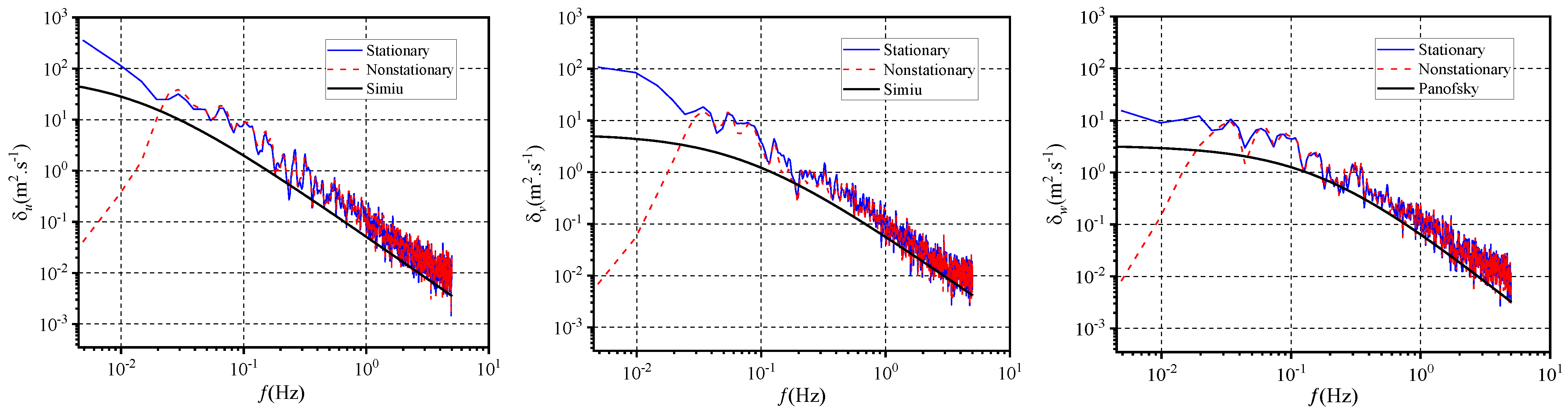
The wind power spectrum assumes an essential function in characterizing the turbulence energy distribution and defining the structure’s dynamic response. Previous scholars have suggested many power spectrums, including the Kamail, Davenport, and Panofsky spectrums, which are suitable for different wind fields. The Chinese wind−resistant design specification recommends using Kamail and Panofsky to estimate the power spectra of the longitudinal and vertical wind speeds, respectively. In this study, the Kamail spectrum, which Simiu modified, is applied to the longitudinal power spectrum. The Kamail power spectrum for longitudinal wind speed under the SWSM is defined as follows:
where is the auto spectrum at height z, is the sampling frequency ), is the friction speed, is the Monin similarity coordinate, and is the constant mean wind speed.
The Simiu-Scanlan power spectrum is utilized for estimating the lateral wind power spectrum as follows:
For evaluating the vertical wind speed, the Panofsky power spectrum is applied, which is calculated as follows:
The power spectrum under the NWSM was evaluated by replacing the mean constant wind speed with the corresponding TVM wind speed.
In this study, the Welch method was applied to estimate the power spectral density of the wind at the corresponding position under both wind speed models. The results were then compared to the Kamail and Panofsky power spectrums, as shown in Figure 16. The figure illustrates that the recommended power spectrums (Kamail and Panofsky) became more consistent with the measured wind power spectrums under medium and high-frequency sections. Furthermore, the measured wind power spectrums in the stationary model were higher than the corresponding power spectrums under the nonstationary model at the low-frequency section, which would affect the prediction of the structure’s dynamic response. While the suggested power spectrums were lower than the power spectrums of fluctuating wind in the stationary model at a low-wind frequency, they were higher than those of the fluctuating wind in the nonstationary model for the same frequency section. These findings agreed with the results reached by other wind observations at complex terrains [21].
4. Conclusions
This study presents a comprehensive analysis of the wind field characteristics at a rocky peak extending from a steep mountainside in complex terrains. A comprehensive examination of the wind properties under the steady and nonstationary wind speed models was conducted. The findings from the field measurements highlighted the significant influence the geographical features of the region have on the wind characteristics at such a location, which resulted in some unexpected outcomes. The conclusions derived from this research were drawn as follows:
- The complexity of the mountainous valley and the peculiarity of the measurement site profoundly influenced the mean wind characteristics; the blocking effect of the local topography resulted in a higher wind angle of attack and lower mean wind speed from the same direction. Furthermore, the probability distribution of the wind field characteristics agreed with the multimodal lognormal distribution;
- The implementation of the reverse arrangement test revealed that the wind speed at the measurement site exhibited strong nonstationary behavior. Additionally, the traditional SWSM overestimated the wind turbulence characteristics. Therefore, the NWSM should be employed to evaluate the wind properties at such topography;
- Due to the speed-up effect imposed on the vertical wind speed, the vertical turbulence integral scale demonstrated a higher value in comparison to the longitudinal and lateral ones. Furthermore, the longitudinal turbulence integral scale was the lowest as a result of the blocking effect that the mountain placed on the upcoming wind flow;
- The power spectrum of the wind fluctuating components complied with the recommended Kamail and Panofsky spectrums at high-frequency stages. Moreover, the wind power spectrums computed via the stationary model were greater than those based on the nonstationary model at lower frequencies.
Author Contributions
Conceptualization, M.N. and F.G.; methodology, M.N.; software, M.N.; validation, F.G. and Q.L.; formal analysis, M.N.; resources, F.G.; writing—original draft preparation, M.N.; writing—review and editing, M.N., F.G. and H.L.; visualization, M.N. and Q.L.; supervision, F.G.; project administration, Q.L. and H.L.; funding acquisition, F.G. All authors have read and agreed to the published version of the manuscript.
Funding
This research was funded by the construction monitoring and technological support unit of the Malukou Zishui Bridge (No: H738012038).
Data Availability Statement
Data will be made available on request.
Conflicts of Interest
The authors affirm that they do not possess any known conflicting financial interests or personal relationships that could potentially influence the findings presented in this study.
References
- Cai, K.; ASCE, S.M.; Huang, M.; ASCE, A.M.; Xu, H.; Kareem, A.; ASCE, A.M. Analysis of nonstationary typhoon winds based on optimal time−varying mean wind speed. J. Struct. Eng. 2022, 148, 12. [Google Scholar] [CrossRef]
- Wang, H.; Wu, T.; Tao, T.; Li, A.; Kareem, A. Measurements and analysis of non−stationary wind characteristics at Sutong Bridge in Typhoon Damrey. J. Wind Eng. Ind. Aerodyn. 2016, 151, 166–182. [Google Scholar] [CrossRef]
- Ren, H.; Laima, S.; Chen, W.L.; Zhang, B.; Guo, A.; Li, H. Numerical simulation and prediction of spatial wind field under complex terrain. J. Wind Eng. Ind. Aerodyn. 2018, 180, 49–65. [Google Scholar] [CrossRef]
- Hu, P.; Han, Y.; Xu, G.; ASCE, A.M.; Li, Y.; Xue, F. Numerical Simulation of Wind Fields at the Bridge Site in Mountain−Gorge Terrain Considering an Updated Curved Boundary Transition Section. J. Aerosp. Eng. 2018, 31, 04018008. [Google Scholar] [CrossRef]
- Li, Y.; Hu, P.; Xu, X.; Qiu, J. Wind characteristics at bridge site in a deep−cutting gorge by wind tunnel test. J. Wind Eng. Ind. Aerodyn. 2017, 160, 30–46. [Google Scholar] [CrossRef]
- Song, J.L.; Li, J.W.; Flay, R.G.J.; Pirooz, A.A.S.; Fu, J.Y. Validation and application of pressure–driven RANS approach for wind parameter predictions in mountainous terrain. J. Wind Eng. Ind. Aerodyn. 2023, 240, 105483. [Google Scholar] [CrossRef]
- Jing, H.; Liao, H.; Ma, C.; Tao, Q.; Jiang, J. Field measurement study of wind characteristics at different measuring positions in a mountainous valley. Exp. Therm. Fluid Sci. 2020, 112, 109991. [Google Scholar] [CrossRef]
- Huang, G.; Jiang, Y.; Peng, L.; Solari, G.; Liao, H.; Li, M. Characteristics of intense winds in mountain area based on field measurement: Focusing on thunderstorm winds. J. Wind Eng. Ind. Aerodyn. 2019, 190, 166–182. [Google Scholar] [CrossRef]
- Jiang, F.; Zhang, M.; Li, Y.; Zhang, J.; Qin, J.; Wu, L. Field measurement study of wind characteristics in mountain terrain: Focusing on sudden intense winds. J. Wind Eng. Ind. Aerodyn. 2021, 218, 104781. [Google Scholar] [CrossRef]
- Bastos, F.; Caetano, E.; Cunha, A.; Cespedes, X.; Flamand, O. Characterisation of the wind properties in the Grande Ravine viaduct. J. Wind Eng. Ind. Aerodyn. 2018, 173, 112–131. [Google Scholar] [CrossRef]
- Liao, H.; Jing, H.; Ma, C.; Tao, Q.; Li, Z. Field measurement study on turbulence field by wind tower and Windcube Lidar in mountain valley. J. Wind Eng. Ind. Aerodyn. 2020, 197, 104090. [Google Scholar] [CrossRef]
- Zhang, J.; Zhang, M.; Li, Y.; Qin, J.; Wei, K.; Song, L. Analysis of wind charactenstics and wind energy potential in complex mountainous region in southwest China. J. Clean. Prod. 2020, 274, 123036. [Google Scholar] [CrossRef]
- Zhou, W.; Lou, W.; Huang, M.; Liu, J.; Liang, M. Two−year wind field measurements near the ground at a site of the Tibetan Plateau. J. Wind Eng. Ind. Aerodyn. 2024, 245, 105636. [Google Scholar] [CrossRef]
- Song, J.L.; Li, J.W.; Flay, R.G.J. Field measurements and wind tunnel investigation of wind characteristics at a bridge site in a Y−shaped valley. J. Wind Eng. Ind. Aerodyn. 2020, 202, 104199. [Google Scholar] [CrossRef]
- Zhang, J.; Zhang, M.; Li, Y.; Jiang, F.; Wu, L.; Guo, D. Comparison of wind characteristics in different directions of deep−cut gorges based on field measurements. J. Wind Eng. Ind. Aerodyn. 2021, 212, 104595. [Google Scholar] [CrossRef]
- Yang, W.; Liu, Y.; Deng, E.; Wang, Y.; He, X.; Lei, M. Characteristics of wind field at tunnel−bridge area in steep valley: Field measurement and LES study. Measurement 2022, 202, 111806. [Google Scholar] [CrossRef]
- Lystad, T.M.; Fenerci, A.; Øiseth, O. Evaluation of mast measurements and wind tunnel terrain models to describe spatially variable wind field characteristics for long−span bridge design. J. Wind Eng. Ind. Aerodyn. 2018, 179, 558–573. [Google Scholar] [CrossRef]
- Yan, B.W.; Li, Q.S.; He, Y.C.; Chan, P.W. RANS simulation of neutral atmospheric boundary layer flows over complex terrain by proper imposition of boundary conditions and modification on the k−ε model. Environ. Fluid Mech. 2016, 16, 1–23. [Google Scholar] [CrossRef]
- Abedi, H. Assessment of flow characteristics over complex terrain covered by the heterogeneous forest at slightly varying mean flow directions: (A case study of a Swedish wind farm). Renew. Energy. 2023, 202, 537–553. [Google Scholar] [CrossRef]
- Li, Y.; Jiang, F.; Zhang, M.; Dai, Y.; Qin, J.; Zhang, J. Observations of periodic thermally−developed winds beside a bridge region in mountain terrain based on field measurement. J. Wind Eng. Ind. Aerodyn. 2022, 225, 104996. [Google Scholar] [CrossRef]
- Huang, P.; Xie, W.; Gu, M. A comparative study of the wind characteristics of three typhoons based on stationary and nonstationary models. Nat. Hazards. 2020, 101, 785–815. [Google Scholar] [CrossRef]
- Yu, C.; Li, Y.; Zhang, M.; Zhang, Y.; Zhai, G. Wind characteristics along a bridge catwalk in (99) a deep−cutting gorge from field measurements. J. Wind Eng. Ind. Aerodyn. 2019, 186, 94–104. [Google Scholar] [CrossRef]
- Ministry of Communications of PRC. Wind−Resistant Design Specification for Highway Bridges, 4th ed.; Tongji University: Shanghai, China, 2018. [Google Scholar]
- Tao, T.; ASCE, S.M.; Wang, H.; ASCE, M.; Wu, T.; ASCE, A.M. Comparative study of the wind characteristics of a strong wind event based on stationary and nonstationary models. J. Struct. Eng. 2022, 143, 5. [Google Scholar] [CrossRef]
- Yan, B.; Chan, P.W.; Li, Q.S.; He, Y.C.; Shu, Z.R. Characterising the fractal dimension of wind speed time series under different terrain conditions. J. Wind Eng. Ind. Aerodyn. 2020, 201, 104165. [Google Scholar] [CrossRef]
- Cheynet, E.; Jakobsen, J.B.; Snæbjörnsson, J.; Mikkelsen, T.; Sjöholm, M.; Mann, J.; Hansen, P.; Angelou, N.; Svardal, B. Application of short−range dual−Doppler lidars to evaluate the coherence of turbulence. Exp. Fluids. 2016, 57, 184. [Google Scholar] [CrossRef]
- Beck, T.W.; Housh, T.J.; Weir, J.P.; Cramer, J.T.; Vardaxis, V.; Johnson, G.O.; Coburn, J.W.; Malek, M.H.; Mielke, M. An examination of the Runs Test, Reverse Arrangements Test, and modified Reverse Arrangements Test for assessing surface EMG signal stationarity. J. Neurosci. Methods. 2006, 156, 242–248. [Google Scholar] [CrossRef]
- Xu, Y.L.; ASCE, M.; Chen, J. Characterizing Nonstationary Wind Speed Using Empirical Mode Decomposition. J. Struct. Eng. 2004, 130, 912–920. [Google Scholar] [CrossRef]
- Yang, H. Experimental Study on Nonstationary Characteristics of Urban Boundary Layer Wind Field. Master’s Thesis, Hefei University of Technology, Hefei, China, 2021. [Google Scholar]
- Jun, F. Non−Stationarity Research on the Measured Signal of Wind−Rain Vibration of Stay Cables Based on Wavelet Analysis. Master’s Thesis, Central South University, Changsha, China, 2010. [Google Scholar]
- Simiu, E.; Yeo, D. Wind Effects on Structures: Modern Structural Design for Wind, 4th ed.; Wiley, National Institute of Standards and Technology: Gaithersburg, MD, USA, 2019. [Google Scholar]
Figure 1.
Real topography at the measurement site.

Figure 2.
Topographical profiles of the terrains at the measurement site.

Figure 3.
Measurement system: (A) 3D ultrasonic anemometer; (B) data collecting and transmitting system.
Figure 3.
Measurement system: (A) 3D ultrasonic anemometer; (B) data collecting and transmitting system.

Figure 4.
Mean wind characteristics: (A) wind rose; (B) local topography; (C) western view; (D) eastern view.
Figure 4.
Mean wind characteristics: (A) wind rose; (B) local topography; (C) western view; (D) eastern view.

Figure 5.
PDF of mean wind speed.

Figure 6.
PDF of wind angle of attack speed.

Figure 7.
Ratios of nonstationary wind speed samples.

Figure 8.
Time−varying and constant mean wind speeds.

Figure 9.
Turbulence intensities based on the SWSM and NWSM.

Figure 10.
PDF of turbulence intensities.

Figure 11.
PDF of the wind gust factor.

Figure 12.
The variation in gust factor with mean wind speed.

Figure 13.
The variation in gust factor with turbulence intensity.

Figure 14.
Turbulence integral scale based on the SWSM and NWSM.

Figure 15.
PDF of the turbulence integral scale.

Figure 16.
Wind power spectral density under the SWSM and NWSM.

Table 1.
Mean turbulence intensity.
| Turbulence Intensity | Stationary | Nonstationary |
|---|---|---|
| Iu | 0.562 | 0.455 |
| Iv | 0.479 | 0.438 |
| Iw | 0.337 | 0.302 |
Table 2.
Mean turbulence intensity based on the steady and nonstationary wind speed models.
| Turbulence Intensity | Stationary | Nonstationary |
|---|---|---|
| Lu | 94.940 | 42.723 |
| Lv | 105.296 | 45.215 |
| Lw | 122.742 | 57.109 |
Disclaimer/Publisher’s Note: The statements, opinions and data contained in all publications are solely those of the individual author(s) and contributor(s) and not of MDPI and/or the editor(s). MDPI and/or the editor(s) disclaim responsibility for any injury to people or property resulting from any ideas, methods, instructions or products referred to in the content. |
© 2024 by the authors. Licensee MDPI, Basel, Switzerland. This article is an open access article distributed under the terms and conditions of the Creative Commons Attribution (CC BY) license (https://creativecommons.org/licenses/by/4.0/).
Share and Cite
MDPI and ACS Style
Nabil, M.; Guo, F.; Li, H.; Long, Q. Mathematical Analysis of the Wind Field Characteristics at a Towering Peak Protruding out of a Steep Mountainside. Mathematics 2024, 12, 1535. https://doi.org/10.3390/math12101535
AMA Style
Nabil M, Guo F, Li H, Long Q. Mathematical Analysis of the Wind Field Characteristics at a Towering Peak Protruding out of a Steep Mountainside. Mathematics. 2024; 12(10):1535. https://doi.org/10.3390/math12101535
Chicago/Turabian StyleNabil, Mohammed, Fengqi Guo, Huan Li, and Qiuliang Long. 2024. "Mathematical Analysis of the Wind Field Characteristics at a Towering Peak Protruding out of a Steep Mountainside" Mathematics 12, no. 10: 1535. https://doi.org/10.3390/math12101535
Note that from the first issue of 2016, this journal uses article numbers instead of page numbers. See further details here.