
Reliability and Residual Life of Cold Standby Systems

1
Department of Basic Courses, Naval University of Engineering, Wuhan 430033, China
2
School of Electronic Engineering, Naval University of Engineering, Wuhan 430033, China
*
Author to whom correspondence should be addressed.
Mathematics 2024, 12(10), 1540; https://doi.org/10.3390/math12101540
Submission received: 18 April 2024
/
Revised: 14 May 2024
/
Accepted: 14 May 2024
/
Published: 15 May 2024
(This article belongs to the Special Issue Mathematical Modelling and Computational Methods in Reliability Engineering)
Abstract
:In this study, we conduct a reliability characterisation study of cold standby systems. Utilising synthetic rectangular formulas and cold preparedness equivalent models for cold standby systems, we analyse the lifetimes of several typical configurations, including series, parallel, and k/n:m voting systems. This study proposes system equivalent models for various types of cold standby systems, all composed of components that follow the same exponential distribution. We use the equivalent model to determine the optimal timing for the use of cold spares and derive the reliability function and residual lifetime function for each type of system. To demonstrate the validity of our model, the Monte Carlo simulation is strategically designed based on the system failure rate function. The experimental results are then compared with those obtained from the numerical model, highlighting that the numerical method incurs a lower time cost.
1. Introduction
A cold standby system is a type of storage system where one or more primary components operate online while additional components remain in standby mode. These systems are characterised by high reliability and low operational costs, making them integral to critical sectors such as aerospace, nuclear power, and high-performance computing systems [1,2]. Thus, analysing the reliability of cold standby systems efficiently is crucial to ensure that their reliability aligns with the design specifications.
Cold standby systems can be categorised into series systems, parallel systems, and voting systems (k/n:m(G) systems). A cold standby series system comprises several functionally identical components arranged in series, supported by multiple cold standby units. When the active components fail, the standby units are activated to replace them, ensuring the system continues to function normally. Yaghoubi and Moradi [3] developed a closed-form equation for the reliability of a system consisting of the main component and (n − 1) cold standby components, utilising the Maclaurin series and polynomial expansion to describe the system’s reliability. Amari and Dill [4] introduced a novel counting process-based method to analyse the reliability of series systems with standby components both efficiently and accurately. In contrast, a cold standby parallel system includes several functionally identical components in parallel, accompanied by numerous cold standby units. These units can replace any failing components flexibly based on the timing of the damage, thereby extending the mean time to failure (MTTF) of the system. Yaghoubi et al. [5] applied Markov’s method to derive the reliability of an (n − k) series standby system, using an exponential distribution to model faults and failures. This approach also led to a closed-form expression for the steady-state reliability of a system with (n − k) cold spares and k parts operating in parallel. Kholief et al. [6] developed steady-state availability equations for three typical cold standby parallel systems using a Markov model. However, these equations were not generalised but tailored specifically to certain systems. Lin et al. [7] formulated a limit state equation for series–parallel cold standby systems by employing an adaptive Markov chain Monte Carlo technique and optimal scaling methods, thereby establishing a comprehensive framework for assessing the reliability of these systems. Zhang et al. [8] examined the reliability model of a parallel system with a single cold standby component, showing that the system’s reliability can be represented as a linear combination of multiple exponential distribution functions, which simplifies the calculations. Wang et al. [9] proposed an approximate model for estimating the reliability of a binary cold backup parallel system based on the central limit theorem. This model was compared with results from the convolution method, demonstrating favourable outcomes. The cold standby voting system (k/n:m(G) system; k-out-of-n) comprises n operating units and m cold standby units, operating normally when at least k units are active. As operational units sustain damage, shifting from n to k, the system will fail upon further damage to the working units. Cold standby units can then be flexibly activated to replace the damaged working units. Wang [10] explored the survival function and the average remaining survival time function of a k-out-of-n system with a cold standby component, using order statistics, the independence of random variables, and the Markov property. Roy and Gupta [11] derived expressions for various reliability functions of the system based on the distribution of component useful life and sequential statistical distributions. Li and Li [12] provided expressions for the survival function and residual life function of a k-out-of-n system with homogeneous components and an independent cold backup component using Archimedean copula theory. Nezakati and Razmkhah [13] applied the maximum likelihood estimation method to estimate the reliability function of a k-out-of-n:F system equipped with a single standby component and obtained asymptotic confidence intervals for this function. The k-out-of-n cold standby system mentioned earlier is essentially a parallel cold standby system with k active components and n-k cold standby components, rather than a dedicated design for k-out-of-n systems with a minimum of k operational components for voting. While references [10,11,12,13] have analysed the reliability of k-out-of-n cold standby systems with one or two spares, practical applications may involve a greater number of cold spares. Therefore, assuming an exponential distribution for each system component, this paper conducts a reliability analysis for k-out-of-n cold standby systems with m cold spares. To facilitate comparison, all methods are categorised in Table 1.
Accurately predicting the remaining life of complex equipment systems holds substantial economic and strategic value, significantly influencing the operation, maintenance, and component replacement of industrial systems. Despite its importance, research on estimating the residual life of cold standby systems, which are typical complex equipment systems, remains insufficient due to their structural complexities. Tuncel [14] introduced the mean inactivity time (MIT) order and the mean residual life (MRL) order to study the residual lifetime of a unitary system equipped with a cold standby unit. Asadi and Bayramoglu [15] explored the average residual lifetime function of a k-out-of-n system at the system level by associating it with the regression relation of the order statistics. Mirjalili et al. [16] utilised the system signature as a basis to study a k-out-of-n system, comparing the stochastic order relationship between the average residual lifetime function of a system and one with a standby component under various conditions, using the system signature method and stochastic ordering theory. Eryilmaz [17] employed the order statistical distribution to present the expression and calculation of the average residual lifetime function of a k-out-of-n:G system with a single cold standby component. Li et al. [18] examined the characteristics of intermittent failures of electrical connectors, establishing a predictive model and method for the remaining life based on the hidden semi-Markov model. Liu et al. [19] determined the number of cold standby units required for a k/n(G)’s system life under different demands using the target operating hours of the system. While these methods can predict the remaining life of the system to a certain extent, most models are not well suited for complex systems due to their computational complexity. To simplify models and calculations, numerical methods are often employed in the prediction of remaining life. Song et al. [20] proposed a numerical method based on Simpson’s formula for predicting the remaining useful life of a system. Zhao et al. [21] approximated the remaining life of a cold standby system using the composite Simpson’s rule (CSR). Karpinski [22] introduced the concept of a residual life set and proposed a general method to determine the distribution of residual life (RSL) of a system following the failure of some components. Chi et al. [23] constructed a confidence interval for the point estimate of the median residual life using a numerical method for left-truncated and right-truncated data. Numerical methods offer an efficient means to compute approximate solutions to complex problems; the results are simple in form, making them easier to implement and interpret compared to analytical solutions. In the realm of electronic system reliability engineering, the acquisition of electronic component failure rates is commonplace. However, in the literature [20,21], the direct application of component reliability functions to calculate the remaining life of complex large systems is inherently limited. Consequently, the broader applicability lies in the direct utilisation of individual component failure rates for such calculations. Furthermore, leveraging the concept of order statistics, this paper establishes the equivalent model of the voting system (parallel system) and presents the system failure rate function graph. Meanwhile, we provide approximate formulas for the reliability function and residual lifetime function of three typical cold standby systems using the composite rectangle method combined with the equivalent model of the voting system (parallel system), offering a reference for their reliability assessments.
In the cold standby parallel system and cold standby voting system discussed earlier, cold standby units can be flexibly activated to replace the operational units of the system upon their failure. Consequently, varying activation times of cold spare parts can influence the reliability and residual life of the system. Zhang et al. [24] explored the optimal allocation strategy of cold spare parts in series and parallel systems. This paper considers a wider range of distribution types, but only compares the system lifespan under two strategies, neglecting intermediate strategies. Li and Li [12] examined the impact of different activation times of a single cold standby part in a k-out-of-n system: activation at the time of a system failure results in the longest system life, whereas activation at the time of the first component’s failure leads to the shortest system life. The study, however, does not provide theoretical proof and focuses solely on scenarios involving a single spare for a given system. Assuming components in the cold standby system follow the same exponential distribution and there is no limit on the number of cold standby components, this study aims to substantiate the theory that the longest system life is attained when the cold standby component is activated at the time of system failure.
The remainder of this paper is organised as follows: Section 2 outlines the basic assumptions and their limitations, the methodology underpinning this research, and the significant distribution models employed in subsequent sections. Section 3 introduces the cold standby equivalent model and supports the conclusion that the longest system life is realised when the system is replaced with spares at the point of failure, alongside an approximation of the reliability function of the cold standby system using a numerical model. Section 4 details the derivation of the system reliability function and residual lifetime function for three types of cold standby systems. Section 5 confirms the accuracy of the numerical model through Monte Carlo simulation. Finally, Section 6 summarises the findings of this study.
2. Assumptions and Theory
2.1. Basic Assumptions
To investigate the reliability and residual life of the cold standby system, this study establishes the following assumptions:
- The system and its components can only exist in two states: a working state or a failure state. There are no intermediate states.
- The focus is solely on the reliability of the working units within the system. The switching time between components is considered negligible, switches are assumed to be completely reliable, and the replacement time of spares is sufficiently brief to be disregarded; thus, normal operations are restored immediately after replacement.
- For any given cold standby system, the life distribution of the system components and cold spare parts follows an exponential distribution. The components operate independently and do not influence each other.
- At any given time during operation, a maximum of one component of the system may fail.
Based on the aforementioned assumption, the scope of systems applicable to this paper is limited to internal components that are mutually independent and follow an exponential distribution, typically electronic components and simple mechanical parts.
2.2. Composite Rectangle Method
The composite rectangle method is utilised in integral calculations. This method involves dividing the domain into multiple subintervals, calculating the rectangular area for each interval, and summing these areas to estimate the integral. This can be expressed by the following equation:
where the integration interval is , the step size is , and are the sub-intervals. As N increases, the number of sub-intervals increases, enhancing the accuracy of the solution. When the sub-intervals are equally spaced (as shown in Figure 1), i.e., , , and , Equation (1) simplifies to the synthesised rectangular formula:
The composite rectangle method has been widely adopted due to its effectiveness. Applying the principles of numerical integration to the analytical expressions of reliability and remaining life significantly reduces computational requirements and enhances the efficiency of predictions.
2.3. Exponential Distribution vs. Gamma Distribution
2.3.1. Exponential Distribution
The exponential distribution is a fundamental life distribution extensively utilised in reliability theory, particularly in the study of electronic products.
Consider an item with a lifetime distribution function:
Here, T is said to follow an exponential distribution with parameter , denoted as . The failure probability density of T is as follows:
For an item whose life follows an exponential distribution with parameter , the MTTF is calculated as follows:
Property 1.
Memorylessness of exponential distribution.
A random variable that follows an exponential distribution exhibits memorylessness, implying that its future behaviour is independent of its past behaviour. Past occurrences do not influence the probability of future occurrences.
2.3.2. Gamma Distribution
A nonnegative random variable follows a gamma distribution, with the following failure probability density function:
This is denoted as , where α and λ are parameters; ; represent Gamma functions; the following gamma functions are involved:
Theorem 1.
(which can be obtained by partial integration) has when is a natural number.
3. Cold Preparedness Equivalent Model and Numerical Estimation Models
3.1. Cold Preparedness Equivalent Models
This section discusses the three types of cold standby systems: the cold standby series system, the cold standby parallel system, and the cold standby voting system. Each system comprises a main system and cold spare parts. The unit lifetimes in these systems are assumed to follow the same exponential distribution with a unit failure rate of . The main system configurations are defined as a k-part series system, an n-part parallel system, and a k/n(G) voting system, complemented by m cold spare parts.
The operation of the parallel system and k/n(G) voting system suggests that the system lifetime is equivalent to the sum of the lifetimes of the following configurations:
(1) Lifetime of an n-unit series system .
(2) Lifetime of an n − 1 unit series system .
(3) Lifetime of an n − 2 unit series system .
……
(n − k + 1) Lifetime of an k unit series system .
Hence, the system lifetime can be described by . This formulation holds for a parallel system of n components when k = 1 ; when , the system behaves as a parallel system.
Owing to the memoryless property of the exponential distribution, the lifetimes are independent. The Laplace transform of the lifetime distribution function of the system can be expressed as follows:
where represents the lifetime distribution function for the lifetime of the i-unit series system. Given that all components in the system adhere to an exponential distribution, the following can be derived from the description in Section 2.3.1:
The system reliability is given by the following equation:
The MTTF of the system, derived from the system life decomposition:
These results are consistent with those found in the literature [25]. Therefore, it is plausible to equate the state changes of the parallel system and the voting system to multiple series systems operating successively.
Next, we introduce cold spare parts, and based on the timing of their activation and the equivalent method previously discussed, the state transfer diagram for the cold standby voting system (parallel system) can be represented as shown in Figure 2.
indicates a state equivalent to units in series; indicates that spares have been used in this state. ; . signifies that the cold spare parts are enabled, and the system returns to the original state immediately after activation. For instance, if a component fails in state and requires transitioning, activating the cold spare results in a transition from to , and after the transfer, the state immediately transitions to , but ; if the cold spare is not activated, then transitions to , and .
Depending on the activation timing of the cold spare parts and the state of the system, the system life can be expressed as follows:
where indicates the time when the first cold spare parts were activated and .
Because are independent, the Laplace transform of the lifetime distribution function of the system can be expressed as follows:
where and . is the lifetime distribution function of the voting (parallel) system and is the lifetime distribution function of the cold spare parts. Furthermore, the failure probability density function of the system can be obtained:
Here, represents the failure probability density function for the system without cold spares activated and is the failure probability density function for the sum of the equivalent series system lifetimes when all cold spares are activated.
In , is constant for parallel and voting systems, but the lifetime distribution function of cold spare parts varies significantly depending on the timing of their replacement, necessitating further investigation of .
Theorem 2.
Given , , and and holds for all x, then > .
Proof.
By comparing the convolution results of the functions and , and given the definition of convolution, we express the following:
(math.) genus .
As , we can denote and as and , respectively, where holds for all .
Then, for and , we have , and . Because , the value of is greater than at each integration point. Therefore, the value of will be greater than . □
Consequently, it becomes apparent that remains constant, while the system’s life in the states following the activation of each cold standby unit can be initiated at any point during the system’s failure process. Therefore, it is only necessary to consider maximizing . Leveraging the properties of convolution, the distribution function of can be expressed as . According to the characteristics of the lifetime distribution function and Theorem 2, the smaller the value of ), the better the reliability of the system’s lifetime. Therefore, the corresponding state of should be , when the value of is considered, and the system life is the longest. It can be further expressed as .
Conclusion 1: In cold standby systems, activating cold spare parts later extends the system life. The shortest system life occurs when system components are replaced immediately upon failure, and the longest when cold spare parts are activated only after the system fails due to component damage.
3.2. Numerical Estimation Model
In this section, using the equivalent model as a basis, the relationship between the remaining life and the failure probability density function is derived. To simplify the integral calculation, the remaining life of the system is numerically predicted using the composite rectangle method.
According to the previous section, the failure probability density function of the system can be expressed:
From this, we can derive the lifetime distribution function and the system reliability function:
As noted in the literature [26], the remaining life expectancy of the system at time is as follows:
Given that the integral exists at , a number close to can be utilised instead. This value () can be assumed based on the number of components and their failure rates. In addressing the issues of step size and accuracy concerning the composite rectangle method, it is essential to consider the specific research subject. In this paper, the primary focus is on electronic components, which are characterised by long lifespans and high reliability. Based on the individual component’s failure rate, we assume the total step size to be , with a single step size of , where N is the sum of the number of all components to facilitate our later calculations.
The time difference between time 0 and t is t; this is divided into intervals; .
Failure probability density function:
Lifetime distribution function:
Reliability function:
The time difference between time t and (∞) is (M − t), which is divided into n2 intervals; .
The approximate solution of the residual lifetime function can be expressed as follows:
When , and can be represented as follows:
Through the above derivation, the integral calculation in the reliability function can be transformed into the product of the summation calculation of the failure probability density function for prediction, which avoids the need to solve the complex reliability formula directly. In this study, the composite rectangle method is applied to simplify the calculation and address the complex integral problems associated with remaining life prediction.
4. Reliability Function and Residual Lifetime Function for Cold Standby Systems
4.1. Cold Standby Series System
In a cold standby series system, if any of the operational units that constitute the system fails, the system itself fails. However, cold spare parts are immediately activated to replace the failed unit, thus restoring the system to normal operation. The components of the system are identical, and their reliability follows an exponential distribution with the parameter . The system comprises components as the main unit, with cold spare parts, and . The reliability block diagram is shown in Figure 3.
In the cold standby series system, the immediate replacement and updating of any damaged part of the main series system ensure the continued normal operation of the system. The state transfer diagram of the cold standby series system is presented in Figure 4.
indicates that the system status is in a state where the -component series system is operating normally and has used cold spare parts. indicates that the system is in a state where cold spare parts are activated to replace failed parts.
The initial state is a -component series system with a lifetime distribution function represented by the following:
Failure probability density function:
Laplace transform of :
In a cold standby series system, there is only one method for replacing cold spares. Based on the system’s operational mechanism, it is understood that the system resumes the state of parts in series after each state. Thus, the lifetime of the system can be described in the following form:
The Laplace transform of the failure probability density function of the system, according to the equivalent model presented in Section 3.1, is as below:
Failure probability density function :
Lifetime distribution function:
Reliability function:
MTTF:
Residual lifetime function:
Due to the complex integral operations required to determine the remaining life, the calculation is more intricate. Therefore, through the numerical model, using a number (M) close to instead of , the time difference between and , , is divided into intervals; .
The residual lifetime function can then be transformed:
In calculating the reliability index of the cold standby series system, complex integrals primarily appear in the derivation of the residual lifetime function. Therefore, only the approximate function of the residual lifetime function is derived.
4.2. Cold Standby Parallel System
In a cold standby parallel system, the system operates normally as long as at least one of the operating units remains functional. Cold spare parts can be activated and replaced at any time, both during and prior to system failure. All components are identical, and their reliability follows an exponential distribution with the parameter . The system comprises n components, forming the main system, supplemented by m cold spare parts.
The reliability block diagram is shown in Figure 5.
According to the cold standby system equivalent model, the system life can be expressed as follows:
Based on Conclusion 1, at the maximum system lifetime can be expressed as the following:
The failure probability density function of the system can be expressed as . Here,
Further computation of , , could not yield an integral-free solution.
Therefore, numerical methods are employed to approximate the solution. The time difference from time 0 to is divided into intervals; . The time difference between time and is , which is divided into intervals; .
Failure probability density function:
Lifetime distribution function:
Reliability function:
Residual lifetime function:
Typically, the step sizes and are set to be the same, i.e., .
Further, the following can be obtained:
In the solution process for the cold standby parallel system, the use of the Gamma function in the derivation of integral calculations introduces complexity. Employing numerical models to approximate the reliability function and residual lifetime function effectively reduces this complexity, thereby facilitating the study of the system’s reliability index.
4.3. Cold Standby Voting System
In a k/n:m(G) cold standby voting system, the system functions correctly if at least of the operating units are working properly. Cold spare parts can be activated and replaced both during and prior to system failure. The components are identical, and their reliability adheres to an exponential distribution with the parameter . The system comprises main components and is supported by cold spare parts. The reliability block diagram is shown in Figure 6.
According to the equivalent model for cold standby systems, the system life can be expressed as follows:
Following Conclusion 1, at the maximum system lifetime can be expressed as below:
The failure probability density function of the system can be expressed as , where
Further computation of reveals that no integral-free solution can be obtained:
Therefore, numerical methods are employed to approximate the solution. The time difference between time 0 and is , which is divided into intervals; . The time difference between time and is , which is divided into intervals; .
Failure probability density function:
Lifetime distribution function:
Reliability function:
Residual lifetime function:
Generally, the step sizes and are set to be the same, i.e., .
Further, we obtain the following:
In this section, the relationship between system reliability and component reliability is calculated for three typical systems, and an approximate function for the system residual lifetime function is obtained. To demonstrate the superiority of the numerical model, we will verify this illustration using three sets of control experiments in the next section to validate this statement.
5. Monte Carlo Simulation
Monte Carlo simulation is an effective method for assessing system reliability [7], and the relevant literature [27,28] has provided specific procedures and pseudocode for system reliability simulation. However, the use of simulation methods to predict the remaining life of a system has only been suggested as a potential application [20,29], without providing specific simulation procedures for other readers to reference. To demonstrate the validity of the numerical estimation model, Monte Carlo simulation experiments are designed in this section to compare and analyse the remaining useful life prediction results.
5.1. Failure Rate Analysis of the System
To conduct a Monte Carlo test rationally and efficiently, the failure rate of each system should be analysed. As mentioned in the previous section, the lifespan of each component within the system follows an exponential distribution. Therefore, according to the characteristic of memorylessness of the exponential distribution, we can determine the failure rate of the component series system.
Based on the state transfer diagram presented in Section 4.1, we can obtain a plot of the failure rate function of the cold standby series system (Figure 7).
Following the method proposed for the equivalent model in Section 3.1, depending on the operating state of the system, we can easily obtain the efficiency function graphs for the cold standby parallel system and the cold standby voting system.
The graph of the failure rate function for the cold standby parallel system is presented in Figure 8; (i = 1, 2 …, n), where m is the number of spares.
The graph of the failure rate function for the k/n:m(G) cold standby voting system is shown in Figure 9; (i = 1, 2 …, k), where m is the number of spares.
The graph of the failure rate function can effectively help us analyse the working state of the system at each time point. In the upcoming step of setting the failure strategy in the Monte Carlo simulation process, it is necessary to effectively integrate the graph of the failure rate function to assess the current failure rate of the system.
5.2. Monte Carlo Simulation Flow Design
In this section, a residual life prediction model based on Monte Carlo simulation is developed. This model takes the failure rates of each component in the system (λ1, λ2 … λn) as inputs and, based on the system model such as series, parallel system, and voting, designs the failure strategy. The specific implementation of the proposed method is shown in Figure 10.
5.3. Comparison of Results
For each system, 100,000 samples are generated, with system internals adhering to an exponential distribution with a failure rate of . Each sample’s internal parts are checked by random sampling. If the system samples fail, then the sample checking stops and the number of checks at failure is recorded. When all samples have failed or T is greater than M , the mean value of T is taken as the residual life prediction of the system. Given the sufficiently large number of samples, the simulation results can be considered approximately accurate.
To ensure comparability, the parameters of both methods are set identically, allowing for both to predict the remaining life of the same system and thus verifying the effectiveness of the proposed method. The configurations for the simulations are as follows: the cold standby series system comprises a three-part series with three cold spares; the cold standby parallel system includes a three-part parallel configuration with three cold spares; and the cold standby voting system is modelled as a 3/5:3(G) system. Figure 11, Figure 12 and Figure 13 show the simulation results for the cold standby tandem system, the cold standby parallel system, and the cold standby voting system, respectively.
Assuming that the cold standby series system consists of a three-part series main system following the exponential distribution with and three cold spare parts, the remaining life of the system after 50 h of operation is predicted. At the end of the model run, the residual life of the cold standby series system was determined to be 89.7713 h.
Assuming that the cold standby parallel system consists of a three-part parallel main system following the exponential distribution with and three cold spares, the remaining life of the system after 100 h of operation is predicted. The residual life of the cold standby parallel system obtained, determined at the end of the model run, is 383.0149 h.
Assuming that the cold standby voting system is a 3/5:3(G) system consisting of a 3/5(G) voting main system following the exponential distribution with and three cold spare parts, the remaining life of the system after 100 h of operation is predicted. The residual life of the cold standby voting system, determined at the end of the model run, was 92.4891 h.
In summary, the remaining life predictions for the three systems using the Monte Carlo simulation method are 89.7713 h, 383.0149 h, and 92.4891 h, respectively. Under the numerical method, the remaining life for these systems is calculated using Equations (39), (46), and (56) as 90.0498 h, 384.30059 h, and 93.0447 h, respectively. The comparative results of the remaining life predictions obtained by both methods are summarised in Table 2.
The comparisons in Table 2 show that the estimated deviations for the cold standby series system, cold standby parallel system, and cold standby voting system are 0.3102%, 0.3357%, and 0.5981%, respectively, all of which are less than 1%. This highlights the sufficient accuracy of the proposed methods. Moreover, the application of the synthetic rectangular formulation in remaining life prediction demonstrates adequate performance, particularly in terms of time efficiency, despite the approximations in the calculations. The operating times for the numerical and simulation methods are detailed in Table 3.
According to the data in Table 3, the numerical method reduces the time cost by more than 60% and up to 99% compared to the simulation method. This is of considerable engineering significance, particularly for the significant reduction in computational costs for highly integrated and complex systems. When dealing with more complex systems such as cold standby parallel systems and cold standby voting systems, it is evident that the performance of numerical models far exceeds that of simulation models. Furthermore, in the case of relatively simple system structures, the efficiency of numerical methods significantly surpasses that of simulation methods.
To further demonstrate the superiority of numerical models, I conducted comparative experiments on similar systems to observe the efficiency improvement brought by numerical methods. The assumed cold standby voting systems for comparison are the 3/5:3(G) system, the 5/7:3(G) system, and the 3/7:5(G) system. The components within the systems follow an exponential distribution with λ = 0.01, and the remaining lifespan of each system after 100 h of operation was predicted. Figure 14 and Figure 15 show the simulation results for the 5/7:3(G) system and the 3/7:5(G) system, respectively.
In summary, the remaining life predictions for the three systems using the Monte Carlo simulation method are 89.7713 h, 43.0623 h, and 175.9736 h, and the time costs are 8.158404 s, 3.827812 s, and 15.933225 s, respectively. Under the numerical method, the remaining life for these systems is calculated using Equation (56) as 90.0498 h, 42.9651 h, and 176.9133 h, and the time cost is 2.459336 s, 0.562434 s, and 3.109148 s, respectively. The comparative results of the remaining life predictions obtained by both methods are summarised in Table 4.
According to the data in Table 3, the numerical model continues to demonstrate superiority over the simulation model in predicting the remaining lifespan of similar cold standby systems, achieving comparable results in a shorter amount of time. Therefore, the numerical model proves to be a very effective solution for predicting the remaining lifespan of cold standby systems.
6. Conclusions
In summary, this study establishes an equivalent model of the cold standby system and substantiates the conclusion that activating cold spare parts at the time of system failure maximises the replacement system’s life. Subsequently, using the synthetic rectangular formula, approximate formulas for the system reliability function and residual lifetime function are derived. Towards the conclusion of this study, a Monte Carlo simulation model for predicting the remaining life of a cold standby system is designed. Through illustrative examples, the results of the numerical method are compared with those of the simulation, highlighting that the numerical method incurs a lower time cost.
The methodology proposed in this study offers a practical solution for predicting the residual lifetime of complex cold standby systems. It allows for the estimation of residual life through the lifetime distribution function or the reliability function of the system’s internal components, thereby simplifying the analytical calculation process and reducing the time cost. The approach is primarily applied to systems where internal components adhere to the exponential distribution, typically electronic components and simple mechanical parts, which tend to have constant failure rates. However, the conclusions and methods obtained still have great limitations. Further investigation is warranted for cold standby systems comprising more intricate components. Therefore, in a forthcoming paper, the intention is to examine various distributions, including the Weibull distribution. Additionally, investigation will be made into scenarios where the components of the primary system follow an exponential distribution, while the cold standby units follow a Weibull distribution. Under these complex conditions, the resulting conclusions may possess a wider range of applicability.
Author Contributions
Conceptualisation, L.L. and X.A.; methodology, X.A.; software, L.L.; validation, L.L., X.A. and J.W.; formal analysis, L.L.; investigation, X.A.; resources, L.L.; data curation, X.A.; writing—original draft preparation, L.L.; writing—review and editing, X.A.; visualisation, X.A.; supervision, X.A.; project administration, J.W.; funding acquisition, J.W. All authors have read and agreed to the published version of the manuscript.
Funding
This research received no external funding.
Data Availability Statement
No new data were created or analysed in this study. Data sharing is not applicable to this article.
Conflicts of Interest
The authors declare no conflicts of interest.
References
- Zhao, Q.; Jia, X.; Cheng, Z.; Guo, B. Bayesian estimation of residual life for Weibull-distributed components of on-orbit satellites based on multi-source information fusion. Appl. Sci. 2019, 9, 3017. [Google Scholar] [CrossRef]
- Cai, X.; Yan, L.; Li, Y.; Wu, Y. Fiducial lower confidence limit of reliability for a power distribution system. Appl. Sci. 2021, 11, 11317. [Google Scholar] [CrossRef]
- Yaghoubi, A.; Moradi, N. An explicit formula for reliability of 1-out-of-n cold standby spare systems with Weibull distribution. Int. J. Reliab. Qual. Saf. Eng. 2023, 30, 2250029. [Google Scholar] [CrossRef]
- Amari, S.V.; Dill, G. A new method for reliability analysis of standby systems. In Proceedings of the 2009 Annual Reliability and Maintainability Symposium, Fort Worth, TX, USA, 26–29 January 2009. [Google Scholar]
- Yaghoubi, A.; Niaki, S.T.A.; Rostamzadeh, H. A closed-form equation for steady-state availability of cold standby repairable k-out-of-n: G systems. Int. J. Qual. Reliab. Manag. 2020, 37, 145–155. [Google Scholar] [CrossRef]
- Kholief, G.; Kholief, E.; Grida, M.; Zaied, A.N. Cold standby system availability. In Proceedings of the 2023 International Telecommunications Conference (ITC-Egypt), Alexandria, Egypt, 18–20 July 2023. [Google Scholar]
- Lin, Z.; Tao, L.; Wang, S.; Yong, N.; Xia, D.; Wang, J.; Ge, D. A subset simulation analysis framework for rapid reliability evaluation of series-parallel cold standby systems. Reliab. Eng. Syst. Saf. 2024, 241, 109706. [Google Scholar] [CrossRef]
- Zhang, Y.; Sun, Y.; Li, L.; Zhao, M. Copula-based reliability analysis for a parallel system with a cold standby. Commun. Stat.-Theor. Methods 2018, 47, 562–582. [Google Scholar] [CrossRef]
- Wang, C.; Xing, L.; Amari, S.V. A fast approximation method for reliability analysis of cold-standby systems. Reliab. Eng. Syst. Saf. 2012, 106, 119–126. [Google Scholar] [CrossRef]
- Wang, Y. Conditional k-out-of-n systems with a cold standby component. Commun. Stat.-Theor. Methods 2016, 45, 6253–6262. [Google Scholar] [CrossRef]
- Roy, A.; Gupta, N. Reliability function of k-out-of-n system equipped with two cold standby components. Commun. Stat.-Theor. Methods 2021, 50, 5759–5778. [Google Scholar] [CrossRef]
- Li, C.; Li, X. On k-out-of-n systems with homogeneous components and one independent cold standby redundancy. Stat. Probabil. Lett. 2023, 203, 109918. [Google Scholar] [CrossRef]
- Nezakati, E.; Razmkhah, M. On reliability analysis of k-Out-of-n: F systems equipped with a single cold standby component under degradation performance. IEEE Trans. Reliab. 2018, 67, 678–687. [Google Scholar] [CrossRef]
- Tuncel, A. Residual lifetime of a system with a cold standby unit. Istat. J. Turk. Stat. Assoc. 2017, 10, 24–32. [Google Scholar]
- Asadi, M.; Bayramoglu, I. The mean residual life function of a k-out-of-n structure at the system level. IEEE Trans. Reliab. 2006, 55, 314–318. [Google Scholar] [CrossRef]
- Mirjalili, A.; Sadegh, M.K.; Rezaei, M. A note on the mean residual life of a coherent system with a cold standby component. Commun. Stat.-Theor. Methods 2017, 46, 10348–10358. [Google Scholar] [CrossRef]
- Eryilmaz, S. On the mean residual life of a k-out-of-n: G system with a single cold standby component. Eur. J. Oper. Res. 2012, 222, 273–277. [Google Scholar] [CrossRef]
- Li, Q.; Lv, K.; Qiu, J.; Liu, G. Research on residual life prediction for electrical connectors based on intermittent failure and hidden semi-Markov model. Appl. Sci. 2018, 8, 1373. [Google Scholar] [CrossRef]
- Liu, H.; Shao, S.; Zhang, Z. Task-based prediction of ship spare parts demand in k/n(G) system. Syst. Eng. Electron. 2021, 43, 2189–2196. [Google Scholar] [CrossRef]
- Song, Z.L.; Zhao, Q.; Jiang, P.; Guo, B. A numerical method for system residual life prediction based on Simpson formula. Commun. Stat.-Simul. Comput. 2021, 50, 4171–4186. [Google Scholar] [CrossRef]
- Zhao, Q.; Tan, Y.; Wu, B.; Jiang, P.; Guo, B. Approximate calculation method for the remaining life of cold standby systems. Syst. Eng. Electron. Technol. 2023, 45, 913–920. [Google Scholar] [CrossRef]
- Karpinski, J. Distribution of residual system-life after partial failures. IEEE Trans. Reliab. 1988, 37, 539–544. [Google Scholar] [CrossRef]
- Chi, Y.; Tsai, T.H.; Tu, Y.H.; Tsai, W.Y. Comparison of several confidence intervals for median residual lifetime with left-truncated and right-censored data. Commun. Stat.-Simul. Comput. 2016, 45, 701–716. [Google Scholar] [CrossRef]
- Zhang, X.; Zhang, Y.; Fang, R. Allocations of cold standbys to series and parallel systems with dependent components. Appl. Stochast. Mod. Bus. Ind. 2020, 36, 432–451. [Google Scholar] [CrossRef]
- Zhang, Z. Reliability Theory and Engineering Applications; Science Press: Beijing, China, 2012. [Google Scholar]
- Asadi, M.; Bayramoglu, I. A note on the mean residual life function of a parallel system. Commun. Stat.-Theor. Methods 2005, 34, 475–484. [Google Scholar] [CrossRef]
- Oszczypała, M.; Konwerski, J.; Ziółkowski, J.; Małachowski, J. Reliability analysis and redundancy optimization of k-out-of-n systems with random variable k using continuous time Markov chain and Monte Carlo simulation. Reliab. Eng. Syst. Saf. 2024, 242, 109780. [Google Scholar] [CrossRef]
- Weng, Z.; Zhou, J.; Zhan, Z. Reliability evaluation of standalone microgrid based on sequential Monte Carlo simulation method. Energies 2022, 15, 6706. [Google Scholar] [CrossRef]
- Liu, J.; Zio, E. System dynamic reliability assessment and failure prognostics. Reliab. Eng. Syst. Saf. 2017, 160, 21–36. [Google Scholar] [CrossRef]
Figure 1.
Isometric composite rectangle method.

Figure 2.
State transfer diagram for cold standby voting system (parallel system).

Figure 3.
Reliability block diagram of cold standby series system.
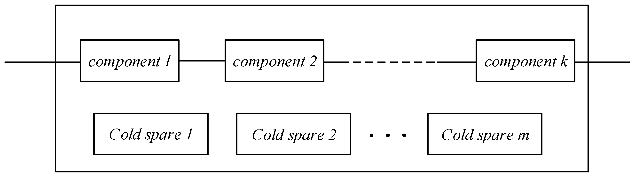
Figure 4.
State transfer diagram for cold standby series system.

Figure 5.
Reliability block diagram of parallel system.
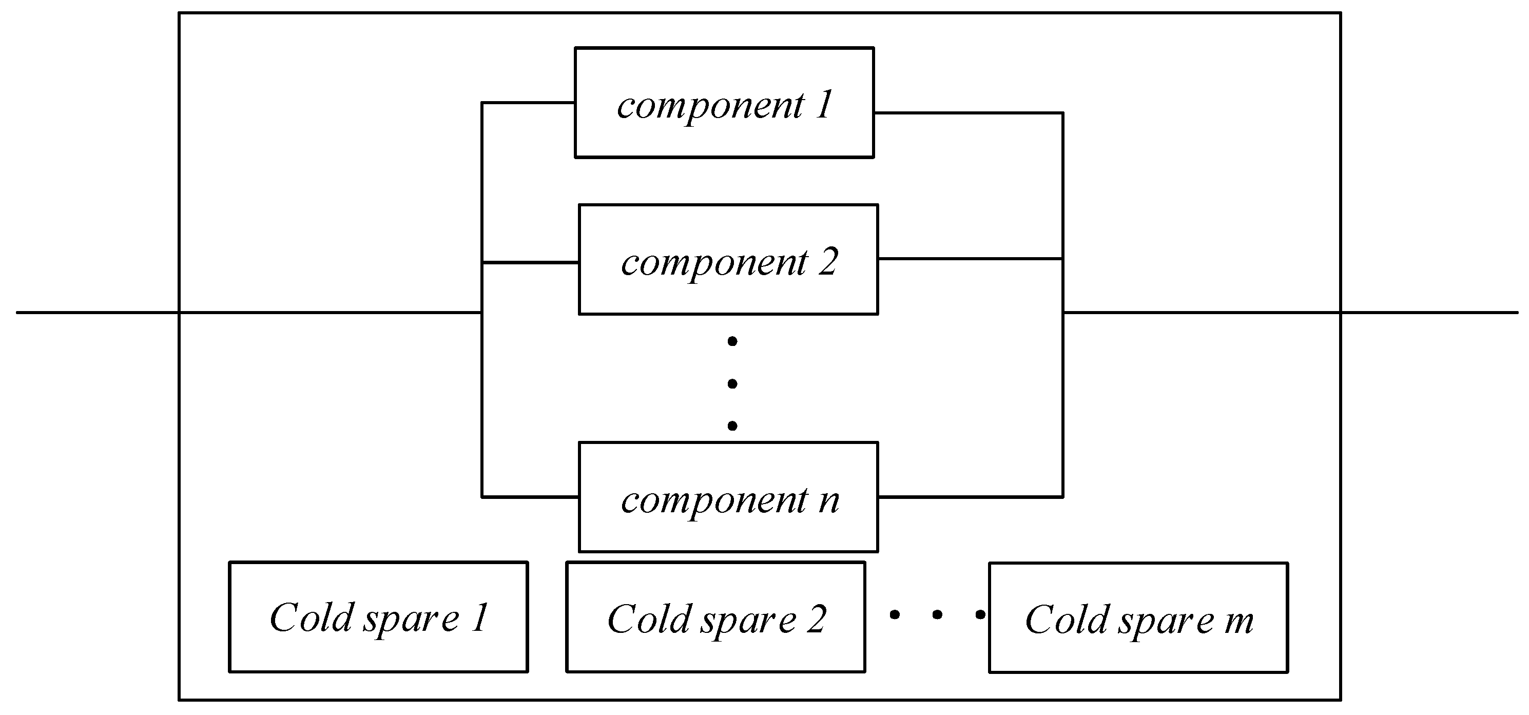
Figure 6.
Reliability block diagram of k/n:m(G) cold standby voting system.

Figure 7.
Failure rate function plot for cold standby series system.

Figure 8.
Failure rate function plot for cold standby parallel system.

Figure 9.
Failure rate function plot for k/n:m(G) cold standby voting system.

Figure 10.
Residual life prediction model based on Monte Carlo simulation.

Figure 11.
Residual life distribution of the cold standby series system based on Monte Carlo simulation.
Figure 11.
Residual life distribution of the cold standby series system based on Monte Carlo simulation.

Figure 12.
Residual life distribution of the cold standby parallel system based on Monte Carlo simulation.
Figure 12.
Residual life distribution of the cold standby parallel system based on Monte Carlo simulation.
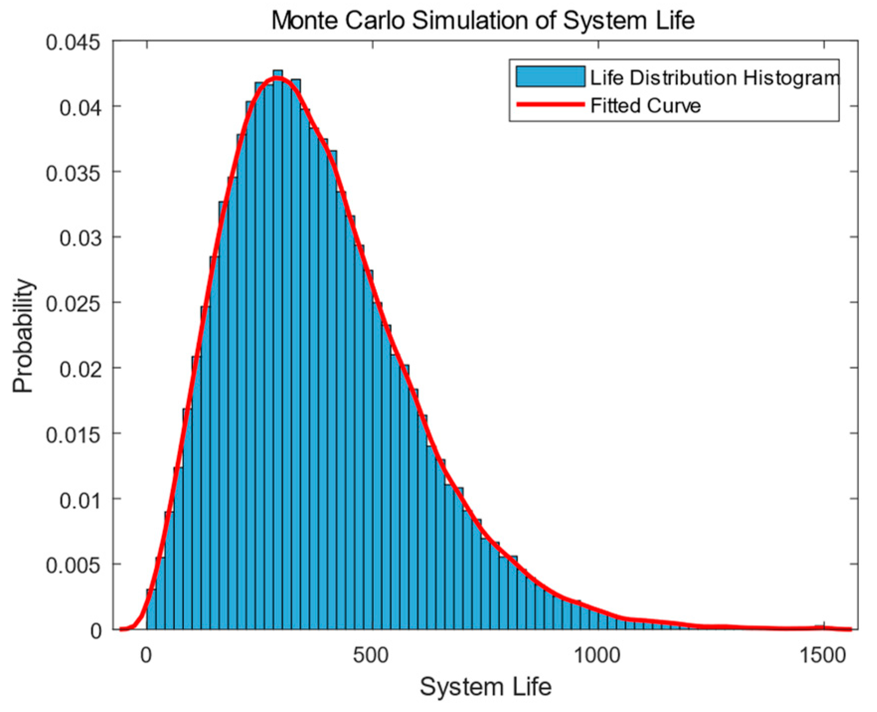
Figure 13.
Residual life distribution of cold standby voting system based on Monte Carlo simulation.
Figure 13.
Residual life distribution of cold standby voting system based on Monte Carlo simulation.

Figure 14.
Residual life distribution of the 5/7:3(G) cold standby parallel system based on Monte Carlo simulation.
Figure 14.
Residual life distribution of the 5/7:3(G) cold standby parallel system based on Monte Carlo simulation.

Figure 15.
Residual life distribution of the 3/7:5(G) cold standby parallel system based on Monte Carlo simulation.
Figure 15.
Residual life distribution of the 3/7:5(G) cold standby parallel system based on Monte Carlo simulation.


Table 1.
Classification of cold storage system calculation methods.
| System Type | Methods | Literature |
|---|---|---|
| Cold Standby Series System | Maclaurin series Counting process | Yaghoubi and Moradi [3] Amari and Dill [4] |
| Cold Standby Parallel System | Markov method Adaptive Markov chain Monte Carlo technique Copula function Central limit theorem | Yaghoubi et al. [5] Kholief et al. [6] Lin et al. [7] Zhang et al. [8] Wang et al. [9] |
| Cold Standby Voting System | Order statistics theory Archimedean copula theory Maximum likelihood estimation (MLE) | Wang [10]; Roy and Gupta [11] Li and Li [12] Nezakati and Razmkhah [13] |
Table 2.
Results of residual life prediction.
| Structure Type | Cold Standby Series System | Cold Standby Parallel System | Cold Standby Voting System |
|---|---|---|---|
| System composition | 3 parts series, 3 cold spare parts system | 3 parts parallel, 3 cold spare parts system | 3/5:3(G) cold standby voting system |
| Time of prediction /t | 50 h | 100 h | 100 h |
| Mean remaining life of the numerical method (h) | 90.0498 | 384.3006 | 93.0447 |
| Mean remaining life of the Monte Carlo simulation (h) | 89.7713 | 383.0149 | 92.4891 |
| Deviation | 0.3102% | 0.3357% | 0.5981% |
Table 3.
Comparison of running time between the two methods.
| Structure Type | Cold Standby Series System | Cold Standby Parallel System | Cold Standby Voting System |
|---|---|---|---|
| The time to run the numerical method (s) | 0.0001116 | 3.508261 | 2.459336 |
| Time to run the Monte Carlo simulation (s) | 7.358136 | 33.430618 | 8.158404 |
| Time cost reduction ratio | 99.9984% | 89.5058% | 69.8552% |
Table 4.
Results of residual life prediction for different cold standby voting systems.
| Structure Type | 3/5:3(G) Cold Standby Voting System | 5/7:3(G) Cold Standby Voting System | 3/7:5(G) Cold Standby Voting System |
|---|---|---|---|
| Time of prediction /t | 100 h | 100 h | 100 h |
| Mean remaining life of the numerical method (h) | 90.0498 | 42.9651 | 176.9133 |
| Mean remaining life of the Monte Carlo simulation (h) | 89.7713 | 43.0623 | 175.9736 |
| Deviation | 0.3102% | 0.2257% | 0.5340% |
| The time to run the numerical method (s) | 2.459336 | 0.562434 | 3.109148 |
| Time to run the Monte Carlo simulation (s) | 8.158404 | 3.827812 | 15.933225 |
| Time cost reduction ratio | 69.8552% | 85.3066% | 80.4864% |
Disclaimer/Publisher’s Note: The statements, opinions and data contained in all publications are solely those of the individual author(s) and contributor(s) and not of MDPI and/or the editor(s). MDPI and/or the editor(s) disclaim responsibility for any injury to people or property resulting from any ideas, methods, instructions or products referred to in the content. |
© 2024 by the authors. Licensee MDPI, Basel, Switzerland. This article is an open access article distributed under the terms and conditions of the Creative Commons Attribution (CC BY) license (https://creativecommons.org/licenses/by/4.0/).
Share and Cite
MDPI and ACS Style
Liu, L.; Ai, X.; Wu, J. Reliability and Residual Life of Cold Standby Systems. Mathematics 2024, 12, 1540. https://doi.org/10.3390/math12101540
AMA Style
Liu L, Ai X, Wu J. Reliability and Residual Life of Cold Standby Systems. Mathematics. 2024; 12(10):1540. https://doi.org/10.3390/math12101540
Chicago/Turabian StyleLiu, Longlong, Xiaochuan Ai, and Jun Wu. 2024. "Reliability and Residual Life of Cold Standby Systems" Mathematics 12, no. 10: 1540. https://doi.org/10.3390/math12101540
Note that from the first issue of 2016, this journal uses article numbers instead of page numbers. See further details here.