Article

Pore Pressure Prediction for High-Pressure Tight Sandstone in the Huizhou Sag, Pearl River Mouth Basin, China: A Machine Learning-Based Approach

by
Jin Feng
1,
Qinghui Wang
1,
Min Li
1,
Xiaoyan Li
1,
Kaijin Zhou
1,
Xin Tian
2,*,
Jiancheng Niu
2,
Zhiling Yang
2,
Qingyu Zhang
2 and
Mengdi Sun
2,*
1
China National Offshore Oil Corporation Limited-Shenzhen, Shenzhen 518067, China
2
National Key Laboratory of Continental Shale Oil, Northeast Petroleum University, Daqing 163318, China
*
Authors to whom correspondence should be addressed.
J. Mar. Sci. Eng. 2024, 12(5), 703; https://doi.org/10.3390/jmse12050703
Submission received: 18 March 2024 / Revised: 21 April 2024 / Accepted: 22 April 2024 / Published: 24 April 2024
(This article belongs to the Special Issue Production Prediction in Onshore and Offshore Tight Reservoirs)

Abstract

:
A growing number of large data sets have created challenges for the oil and gas industry in predicting reservoir parameters and assessing well productivity through efficient and cost-effective techniques. The design of drilling plans for a high-pressure tight-sand reservoir requires accurate estimations of pore pressure (Pp) and reservoir parameters. The objective of this study is to predict and compare the Pp of Huizhou Sag, Pearl River Mouth Basin, China, using conventional techniques and machine learning (ML) algorithms. We investigated the characteristics of low-permeability reservoirs by observing well-logging data sets and cores and examining thin sections under a microscope. In the reservoir zone, the average hydrocarbon saturation is 55%, and the average effective porosity is 11%. The tight sandstone reservoirs consist of fine- to extremely fine-grained argillaceous feldspathic sandstone. The mean absolute error for reservoir property prediction is 1.3%, 2.2%, and 4.8%, respectively, for effective porosity, shale volume, and water saturation. Moreover, the ML algorithm was employed to cross-check the validity of the prediction of Pp. Combining conventional and ML techniques with the core data demonstrates a correlation coefficient (R2) of 0.9587, indicating that ML techniques are the most effective in testing well data. This study shows that ML can effectively predict Pp at subsequent depths in adjacent geologically similar locations. Compared to conventional methods, a substantial data set and ML algorithms improve the precision of Pp predictions.

1. Introduction

The challenges encountered during drilling under uncontrolled pressured conditions can result in well abandonment, incurring substantial costs for hydrocarbon production [1,2]. Companies have made significant efforts to improve pore pressure (Pp) prediction in drill planning to mitigate these risks [3]. The accurate prediction of Pp and assessment of fluid flow play a crucial role in developing hydrocarbon areas, particularly in the well-planning phase [4]. According to a survey conducted on 2520 wells completed in the Gulf of Mexico, problems with gas flow, shallow water flow, kicks, and lost circulation accounted for more than 24% of the entire drilling duration. These problems were primarily related to the fracture inclination and imprecise pore pressure estimation [5]. A robust modeling approach is required to precisely predict shear stress for the thixotropic fluids because these fluids have widespread use in the petroleum industry due to their prevalence in porous media and pipelines, and their complex rheological behavior [3]. It is crucial to accurately determine the minimum miscibility pressure of the reservoir fluid, rock, and thermal conditions to assess the gas injection process [6,7].
Well-logging data can offer an effective tool to obtain extensive details on subsurface formation and rock properties. Well logs provide such information as lithology information, formation resistivity, clay content, porosity, rock density, water saturation, rock physics, and flow capacity, which are very important for reservoir characterization [8,9,10,11]. Estimating Pp from borehole data has been accomplished through established theoretic techniques, which originated from the Terzaghi and Biot effective stress law [12,13,14,15], to accurately estimate Pp in formations, ensuring safe drilling operations and reducing the environmental effect. Drilling plans are guided by Pp, defined as the fluid pressures within pore spaces of permeable geological formations [4]. Substantial engineering catastrophes, such as seabed instability, formation destruction, well blowouts, etc., typically arise from errors in predicting Pp [16].
Hottmann and Johnson [17] introduced a typical theoretical approach for predicting Pp with shale character derived from sonic (DT) and gamma-ray (GR) logs. This method detected abnormal Pp by identifying deviations from the standard porosity style in the calculated results. Incorporating the average overburden stress gradient, normal fluid pressure gradient, depth, and two empirical constants, this model facilitated rapid Pp prediction. Eaton [15] proposed a renowned classical theoretical equation using Rt data and, later, in 1975, introduced a new empirical equation for Pp prediction utilizing DT data. In this new empirical Eaton model, the DT in the normal trend became a crucial parameter for calculating Pp [16]. Luo et al., 2021, presented a novel Pp model based on GR and resistivity logs’ data set, effective in formations with diverse lithologies and different tectonic compressions [18]. Like the DT-related equation, their empirical equation derived porosity from empirical expressions.
The prediction of Pp is a crucial factor in determining the effectiveness and cost-effectiveness of drilling operations and effectively managing the well. It is considered primary data for petroleum exploration and development strategies. This will aid in mitigating issues related to drilling operations and reducing the associated costs and risks [19,20]. The prediction of Pp has been performed through several traditional methods, which include analytical and numerical approaches. The empirical methods seldom consider the relationships between Pp and other well-log data, including sonic velocity, porosity, and resistivity logs, and the use of these methods makes them frequently utilized in the industry. The empirical methods are subject to some limitations, especially when the correlation is derived from a restricted data set as well as the geological context [20,21,22]. ML algorithms were employed to predict Pp and used risk identification for complex conditions. Nowadays, machines and deep learning-based methods have been developed to precisely predict Pp in cost-effective ways and reduce processing time [13,20].
As a critical region for petroleum production, the Huizhou Sag contains multiple significant hydrocarbon accumulations, especially natural gas reserves like HZ25-7, HZ21-1, LH11-1, and LF13-2. In this basin, grabens and half-grabens created by the Cenozoic extensional fault networks are typically filled with the source rocks [23]. This Cenozoic extension significantly impacts the integrity of fault seals and the preservation of traps [24]. Thus far, exploration efforts have largely penetrated the petroleum targets in the shallower sediments. It has been concluded from a literature review that minimal work was performed on Pp prediction. This study aims to fill this gap by determining the Pp of the basin so that drilling operations can be facilitated.
This research primarily focuses on the tight sandstone reservoirs of the formations in the Huizhou Sag, Pearl River Mouth Basin (PRMB), China. It aims to investigate the reservoir properties and Pp to understand its potential for further exploration and production (E&P) activities. This study addresses the gap in estimating Pp and reservoir properties through conventional and ML approaches with core data calibration. The supervised ML approach offers an innovative alternative for precisely and effectively predicting Pp and characterizing reservoir properties. The random forest (RF) algorithm was employed for a petrophysical analysis, while gradient boost and ADA boost algorithms were utilized for Pp prediction. To facilitate and calibrate ML model results in core data, analyses such as thin-section observation, mineral identification, and porosity and pressure data analyses were performed to investigate the petroleum characteristics of the Wenchang Formation (WC 421).
This study provides valuable insights into predicting Pp through theoretical and ML models and reservoir characterization in the Huizhou Sag Field, utilizing lab-measured formation Pp and readily available conventional well-logging data from the Wenchang Formation. Current research outcomes contribute to a reliable and better understanding of tight reservoirs and enhance our knowledge about Pp prediction from the well log data set. Additionally, these insights provide crucial guidance for oil and gas E&P activities for safe drilling operations in the PRMB, China.

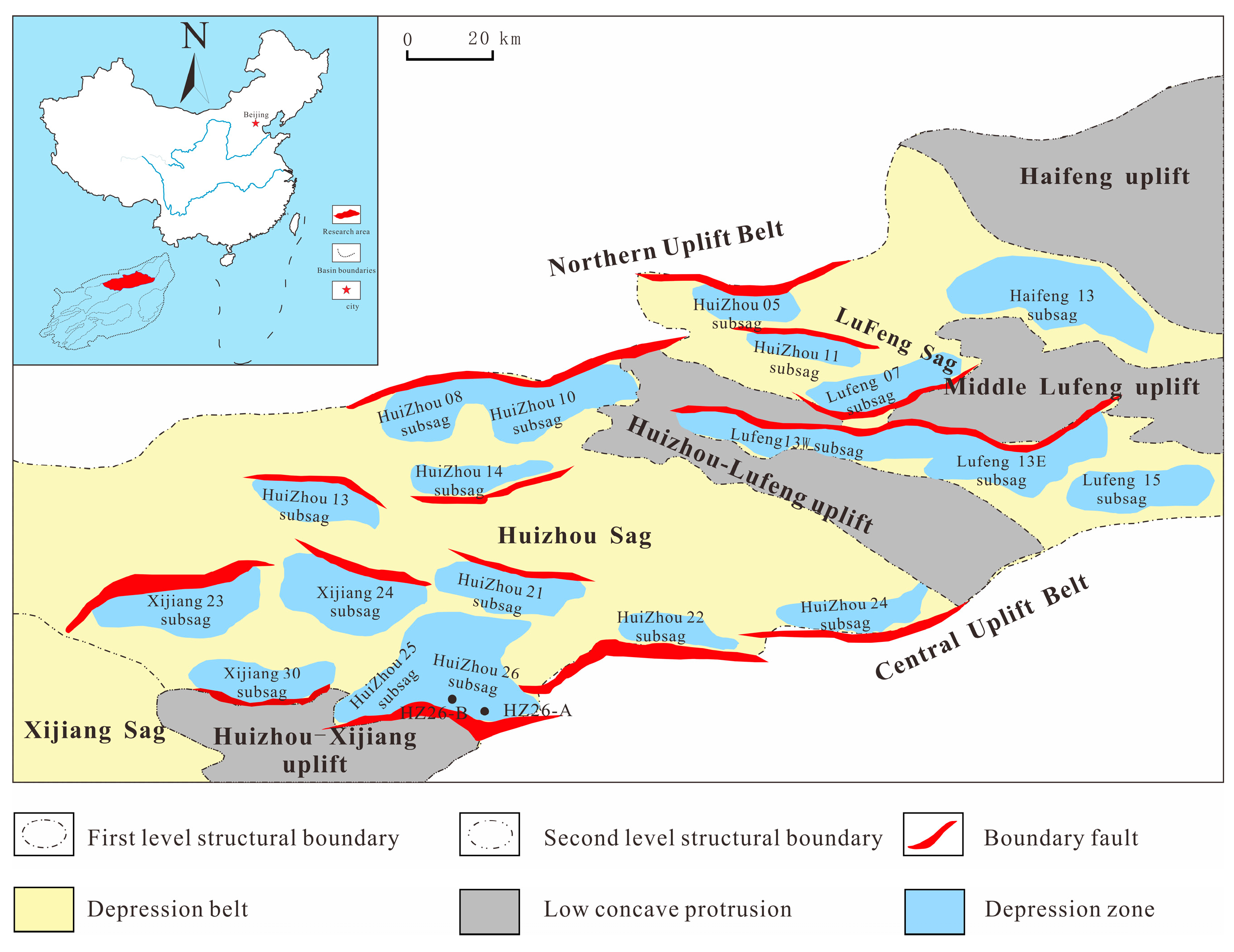
2. Geological Setting

Rift basins are prevalent geological features, among many of which have suffered multiple phases of tectonic activity, incorporating extension, strike-slip, or inversion deformation in various orientations [23,25]. Underneath conditions of extension, newly formed fault systems verge toward being oriented practically vertically to the orientation of the extension fault [18]. However, the resulting fault network becomes more intricate when two extension stages occur in separate directions. This can include curved, various sets of a strike, and intersecting faults, as demonstrated in sandbox analog models [26].
Normal faults are typically generated in large numbers in rift basins during the syn-rift phase. However, their movement is periodic and relatively too constant. These faults may originate in the initial stages of rifting, become inactive during certain sedimentary phases, and then become reactivated and increase due to extensional stresses during later sedimentary periods. Newly formed faults that initiate during the late deposition phase may generate downward, vertically linking with other initial-manufacture faults or developing separately [18,27].
As a result, newly generated faults connected to reactivated faults are less affected by older faults and may display variations in their direction and propagation. The PRMB is a vast offshore sedimentary basin that spans around 175,000 square kilometers along the South China Continental border. That includes a sedimentary sequence of up to 17 km in depth, composed of Cenozoic and Mesozoic fluvial to marine deposits, including carbonate and clastic strata. The basin exhibits a complicated structural configuration, with different uplifted regions split by dual bowl shape geometry running in a NEE-SWW orientation (as shown in Figure 1). The northern depression zone comprises the Zhu 1 and Zhu 3 depressions. Comparatively, the southern depression was formed by the Zhu 2 and Chaoshan depressions. The Zhu 1 depression, located at the heart of the Huizhou Sag, extends over 11,719 sq. kilometers with a depth of around 10,000 m. Given the significance of this region, it is crucial to identify additional petroleum geometry within the basin, reduce exploration uncertainties, and establish dependable geological models for the fault systems in the area.
The literature survey of the study area suggested that the limited exploration data set of the Wenchang Formation is available to establish relationships between sedimentary facies and key formation evaluation parameters for reservoir characterization and enhance drilling operations. The significant post-depositional erosional events, including tectonic inversion and shifts in tectonic patterns, have impacted the Wenchang Formation (Target Formation) composition, and made it heterogeneous, while it was initially deposited in a deeper lake environment [26,28,29,30]. The reservoir formation presented in the study area exhibits distinct facies-controlled characteristics that make the assessment and prediction of reservoir quality viable [31,32]. It has been witnessed that previous studies performed on the Wenchang Formation have primarily focused on examining the structure, resource potential assessment, and source rock evaluation through seismic, well logs, and core data sets, and no study has been reported to predict pore pressure (Pp) of this formation [26,28]. Core measurement is the most reliable method to access reservoir properties and Pp. Still, it is expensive, and limited interval availability makes it challenging to assess the whole reservoir unit potential. To overcome this, the prediction of reservoir quality, Pp, and the potential presence of hydrocarbon in wells can be achieved by well-logging data without core data. Nevertheless, little work has been reported in the study area regarding the comprehension of Pp and a petrophysical analysis through machine learning (ML) methods.
PRMB in the South China Sea, with its two-kilometer-thick layer of Eocene sediments, has emerged as a hotspot for oil exploration. Recent discoveries, like the HZ25-7 field in the Wenchang Formation, have fueled this interest [28]. PRMB, a Cenozoic rift basin stretching northeastward along the continental margin, is crisscrossed by three fault systems: NE-EW normal faults, NW shear faults, and WNW oblique-slip faults [33]. The Huizhou Sag, a shallow area on the continental shelf, has been studied previously. These studies classified the Cenozoic sediments in the Huizhou Sag into syn-rift and post-rift mega-sequences. The syn-rift sequence comprises the Wenchang and Enping formations, divided by the T70 breakup unconformity. The post-rift sequence includes the Zhuhai, Zhujiang, Hanjiang, Yuehai, and Wanshan formations. Figure 2 illustrates Huizhou Sag’s stratigraphy with details on petroleum potential, lithology, and sedimentary facies.

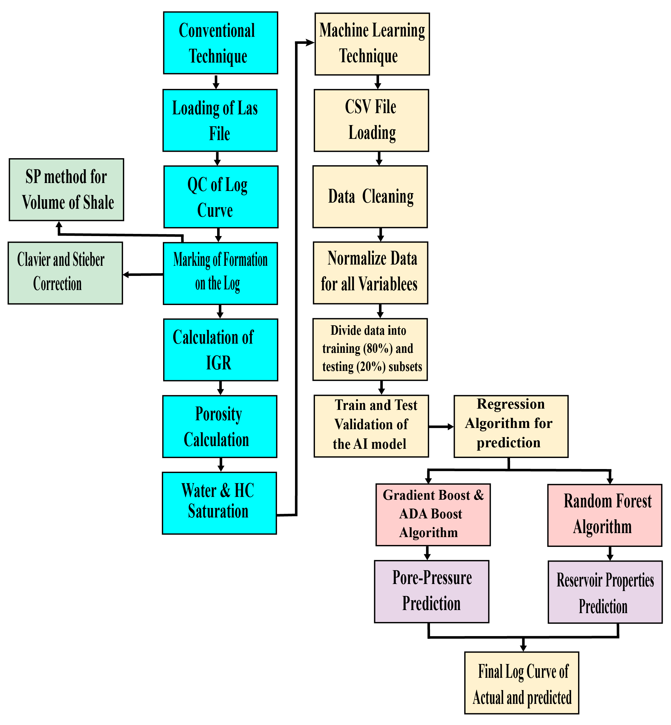
3. Material and Methodology

The present research used data from HZ-26-A in China for reservoir characterization and pore pressure prediction. The log is used for the calculation of parameters. The target zone for the reservoir and pore pressure prediction for HZ-26-A is 3820.15 m to 3837.98 m, and the overall thickness of the zone is 17.83 m. The lithological identification was performed through thin sections (using a German Leica polarizing microscope), and logging equipment was widely used in the geoscience of well HZ-26-A. The sampling and analysis were carried out in strict accordance with the requirements of geological design and on-site geological supervision to identify thin lithology sections in this well, as demonstrated in Figure 3. Present studies employed different types of techniques involving conventional and machine learning approaches.

3.1. Conventional Method

With the help of a traditional linear technique, the volume of shale is estimated, as shown in Equation (1) [35].
I G R = G R log G R cln G R s h l G R cln
V S H C l a v i e r = 1.7 3.38 ( I G R + 0.7 ) 2
V S H S t i e b e r = I G R 3 2 I G R
where I G R is an Index Gamma Ray, GRlog is a log curve value obtained from the gamma-ray log, GRcln is the average minimum value of GR, and GRshl is the maximum value of GRlog. After the calculation of the I G R , the Clavier and Steiber correction was estimated with the help of Equations (2) and (3) [36,37]. The estimation of shale volume through the linear approach, which is not based on geographical features (gamma-ray index), leads to the over-estimation of shale volume values. To reduce this, non-linear approaches have been developed that are more optimistic and reliable [33]. Clevier’s and Steiber’s non-linear approaches rely on geographical features or formation age to improve the accuracy and reliability of shale volume estimation in shaly sand reservoirs [38]. A literature survey revealed that the best estimation of shale volume is obtained using a gamma-ray log with the Stieber non-linear approach, which is calibrated with XRD in the tight reservoir [8]. Therefore, in the current study, we use Steiber’s approach to compute shale volume.
The next step was the calculation of the effective porosity. Effective porosity is the sum of all interconnected pores within the reservoir. The formula for the calculation of effective porosity is shown in Equation (4) [39].
P H I E = P H I A × ( 1 V S H )
In the above equation, PHIE represents the effective porosity, PHIA represents the average porosity, and VSH shows the volume of shale. The last step of petrophysics is the calculation of water saturation; for that, Archie’s equation was used, as shown in Equation (5) [40].
S W A r c h i e = a R w P H I E m R t 1 n
In S W A r c h i e , the saturation of water is calculated using Archie’s equation. Rw is the resistivity of the water, and Rt is the deep resistivity.
Vertical stress (σv) or overburden is the quantitative weight of the sedimentary column that creates the overburden [4,41,42]. Based on the information that is accessible, bulk density and depth data, the overburden can be computed [43]. Equation (6) [44], which shows how to apply the Amoco method to calculate the vertical stress gradient (OBG), uses Z as the depth, RHOB as the bulk density log value, and g as the gravitational acceleration.
O B G = 0 z R H O B ( Z ) g d Z
The effective stress rule of Terzaghi and Biot [45] serves as the foundation for predicting pore pressure. The framework of this theory states that total and vertical effective stress are functions of fluid pore pressure. Equations (7)–(12) were adopted from [15,46] and express the connection between these terms:
Approximation of the normal compaction trend line (NCT).
P p g = σ υ g ( σ υ g P h g ) Δ t n Δ t m
Δ t n = Δ t m ( Δ t m l Δ t m ) e c z
(1)
Calculation of lithostatic pressure.
σ υ g = P s e a + 0 Z ρ b ( Z ) g d Z P s e a Z = 0 Z ρ b ( Z ) g d Z Z g
(2)
Calculation of hydrostatic pressure.
P h g = P s e a + ρ w g Z P s e a Z = ρ w g
(3)
Estimation of pore pressure using Eaton’s equation.
P p g = σ ν g ( σ ν g P h g ) Δ t n Δ t m
P f = P s e a + P p g Z
Δtm is the transit time in the shale matrix, Δtml is the transit time at the mudline (Z = 0), (Z is the true vertical depth below the mudline, (c is the compaction parameter, σe is the effective stress [46], pf is the pore pressure, ppg is the pore pressure gradient, σvgσ is the overburden pressure, phg is the hydrostatic pressure gradient, and Ppg is the formation pore pressure gradient [16,47].

3.2. ML Method

In conventional techniques, different log curves are predicted with the help of a regression analysis. The random forest ML technique was used for the prediction of petrophysical calculation. The detailed methodology of the ML techniques is shown in the flow chart in Figure 4.
In ML techniques, the first step is frequency distribution, which assists in a better understanding of the parameters present in our selected reservoir formation. The frequency distribution chart was developed for petrophysics’ input and output parameters. The plot’s x-axis represents the original scale, and the y-axis represents the frequency distribution, illustrating the frequency range in which different data sets are present, as shown in Figure 5. A pair plot is shown in Figure 6 before the outlier is removed. Note that the outliers were removed by applying the absolute square method. The standard equation available literature was used to calculate the error parameters. The error was calculated by using Equations (13)–(15). A command was given to the code to generate the error parameters.
R M S E = 1 n s a m p l e s i = 0 n s a m p l e s 1 ( y m e a s u r e d , i y p r e d i c t e d , i ) 2
M S E = 1 n s a m p l e s i = 0 n s a m p l e s 1 ( y m e a s u r e d , i y p r e d i c t e d , i ) 2

3.3. Pore Pressure Prediction Using Sonic Log

Pore pressure prediction using a sonic log was performed on the ML algorithm using a sonic log. The input log is shown in Figure 7, along with their calculated parameters like porosity. The blue line shows the sonic log, and the black line represents the GR log. The two shades are marked on the GR log, which shows the shale and sand. Yellow represents the sand facies, and grey demonstrates the shale facies. Figure 8 illustrates the normal compensation line drawn on the sonic log and shown in red. The black scatter plot shows the travel time.
Pp was predicted with the help of gradient boost and ADA boost algorithms. Gradient boosting, being a mean algorithm, might promptly overfit a training data set. Regularization methods, penalizing various algorithm aspects, can enhance performance by controlling overfitting. AdaBoost, also called Adaptive Boosting, is a group ML method that may be used for multiple regression and classification tasks. A supervised learning technique classifies data by combining many weak or base learners (like decision trees) into a robust learner. ADA boosting gives training data set instances weights determined by how well previous classifications performed.

4. Results and Discussions

In recent decades, ML models have been used to predict petrophysical properties more precisely and efficiently because petrophysical properties are industry practice to evaluate the reservoir formation hydrocarbon potential and are further utilized to predict rock physics attributes [47]. The primary reservoir parameters porosity and permeability prediction have been achieved using ML and statistical regression tools in recent years. The use of conventional well-log data with the calibration of core measurements has become particularly effective. ML tools are widely used to accurately estimate reservoir properties, particularly permeability and porosity [48]. To create sophisticated predictive ML models for Pp prediction using petrophysical data [49]. The primary focus of the current study is on the best way to design and use ML models for petrophysical parameter estimation because they are further used to predict Pp.

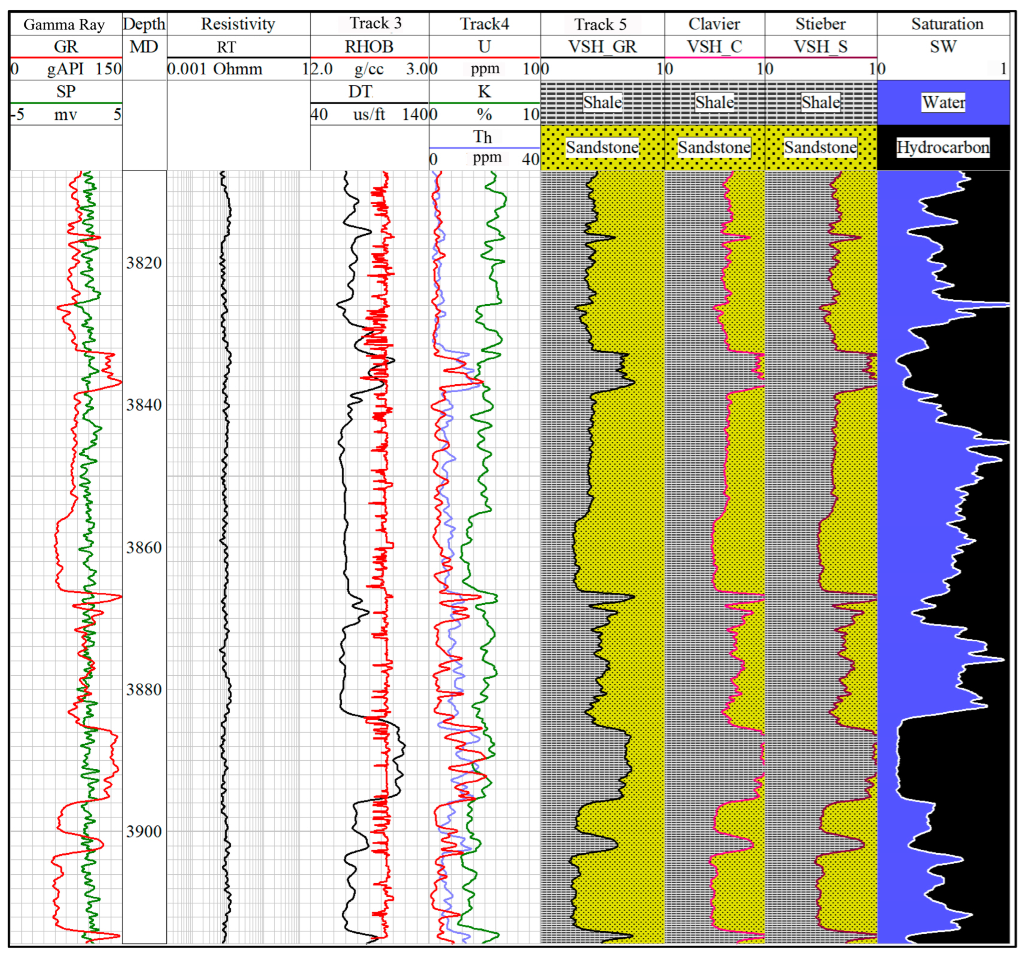
4.1. Conventional Technique
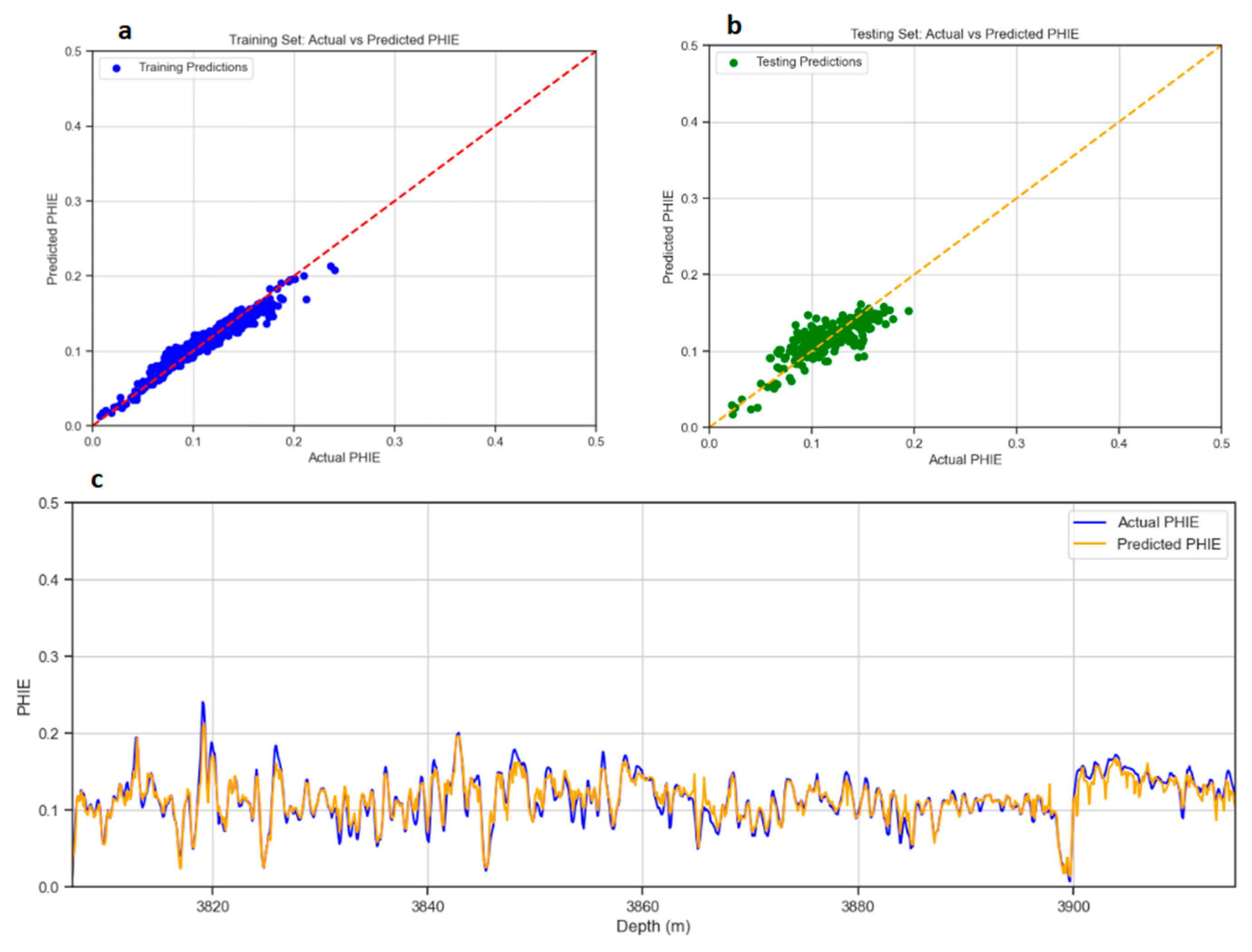
Tight sandstone reservoir assessment is challenging due to their complex diagenesis and considerable heterogeneity in accessing porosity and permeability values. It is a crucial factor that serves as the foundation for creating geological models for the precise estimation of oil and gas reserves and the formulation of sensible development strategies. These days, several mathematical regression and ML techniques on petrophysical data are the primary methodologies for high-precision porosity and permeability prediction. Thin-section petrography and geometric analyses are very helpful in examining the pore structure properties of tight sandstone reservoirs [31,50]. The details of the lithological thin-section identification results of well HZ26-A (drilling coring) are shown in Table 1 to access the tight sandstone reservoirs. The detailed petrophysical analysis result is shown in Figure 9. The correlation track represents the gamma ray with red and SP log with green, and the resistivity track shows the resistivity log, a deep resistivity log curve in a cyan color. The porosity track shows the sonic log curve, and DTR stands for delay time from the receiver. Tracks 5 to 10 show the calculated results. The detailed result of the reservoir formation is shown in Figure 9 and Table 2.
Many clay minerals, including kaolinite, illite, and chlorite, were found in tight sandstone reservoirs, and their presence significantly impacts the quality of the reservoir. The type of clay minerals was determined using a spectral gamma-ray (SGR) log [51,52]. The precise assessment of mineral composition is crucial for enhanced reservoir characterization. However, it presents significant difficulties in shale and tight units because of the intricate mineralogical structure, minimal porosity, and extremely low permeability. Lab measurements can be accessed more precisely [53]. The conventional practice used for the assessment of porosity is lab-based measurement of rock samples as well as traditional logging methods, which encounter constraints related to cost, and time. To address this limitation, a machine learning-based method has been employed for estimating porosity based on drilling data [47,54]. Figure 10 shows the cross plot between the potassium and thorium, representing the amount of minerals present in the reservoir formation.

4.2. ML Techniques

The detailed result of the ML technique is shown in Figure 11, Figure 12 and Figure 13, while Table 3 demonstrates the detailed statistics of the log curve. Figure 11, Figure 12 and Figure 13 represent the correlation between the input parameters of shale volume, PHIE, and saturation and the calculated parameter. Table 4 describes the error result of the calculated parameter. Figure 11, Figure 12 and Figure 13 show the prediction result based on random forest algorithms. The testing and training results vary from the estimated curve data. Figure 11, Figure 12 and Figure 13 show the results of PHIE, SW, and VSH_S, respectively; the testing and training results are green and blue in color, respectively, and the regression line is orange. Most data points lie near the regression line, representing a good testing and training result. The x-axis shows the actual parameters, and the y-axis represents the predicted parameters. The curve is made by each parameter, which represents the actual and predicted parameters corresponding to their depth.

4.3. Pore Pressure Prediction Result

Figure 14 shows the prediction of the Pp by using the conventional method. Five different tracks are present, which represent the different log curves. The Pp is shown in green in the last column, and overburden pressure is shown in red while hydrostatic pressure (HP) is blue. If the HP is greater than the Pp, it is overpressure. Figure 15 shows Pp prediction using ML by the sonic log. The first two tracks represent the input parameters for predicting Pp and the last two tracks represent the Pp prediction result. Different curves are plotted on these tracks; the red in the last track represents the Pp, the blue color demonstrates the lithostatic pressure, and the green color shows the HP. Generally, if the lithostatic pressure is less than the Pp, it is considered an overpressure zone. In contrast, it is regarded as an under-pressure zone if it exceeds the Pp.
Figure 14 and Figure 15 show the Pp prediction of the interested formation in HZ-26-A. The output of Figure 14 is generated with the help of conventional software, while Python algorithms calculate the output of Figure 15. The initial track shows the input parameter for the pressure prediction, and the last two tracks represent the Pp result. The grey color in track 4 shows the sonic log, and the red represents the normal compensate trend line. Track 5 shows the pore pressure prediction in which the blue line represents the hydrostatic pressure, and the green color shows the Pp. If the Pp is greater than the hydrostatic pressure, it represents the overpressure. If hydrostatic pressure is greater than the pore pressure, it shows under-pressure. The machine learning results are better than those of conventional techniques. Figure 16 demonstrates the heat map in which the correlation between different parameters and Pp is defined, showing a correlation of 84% between the sonic log and Pp.
Figure 17 and Figure 18 represent the Pp prediction using gradient boost and ADA boost regression algorithms. Both algorithms give the best prediction of Pp and the best match of correlation between the training and testing data. The green color shows the predicted pressure, while the red color shows the actual pressure. Figure 19 shows the core and predicted pressure using ML and conventional techniques. The R2 calculated by the traditional method is 0.85, while the R2 from the ML method is 0.95 in the testing well. The result of R2 shows that the Pp prediction of machine learning is excellent as compared to a conventional technique. Figure 20 shows the testing of the Pp in blind well HZ-26-B. The first three tracks show the training well parameter and tracks 4 to 6 show the testing well parameter. The prediction is made on the blind well with the R2 of 0.98. Track 7 shows the result of both the training and the blind well. The grey color represents the prediction made on the blind well, and the red color represents the actual training curve. Figure 21 demonstrates the cross plot of predicted versus actual pore pressure with the square regression of 0.98 on the blind well.
It has been inferred based on the literature survey that studies on the prediction of Pp taking into account various ML models are minimal and obtain popularity due to better performance than conventional theoretical models (e.g., Eaton’s method) in geosciences to enhance drilling operations to overcome well failure [22,55]. A heterogeneous lithology presented ML models for Pp prediction that take advantage of well-log curve inputs (sonic velocity, porosity, and shale volume) and depend on geological formation composition [56,57,58]. The following ML techniques were assessed: a support vector machine (SVM), gradient boosting, MLP neural network, and RF were employed to predict Pp as input of petrophysical logs computed from well-log data sets. To precisely estimate Pp, a set of petrophysical data sets is required through a multivariate prediction model. However, in heterogeneous lithologies, the parametric multivariate models with assumptions on lithology require a calibration procedure [59]. Yu et al.’s [57] findings suggested that Pp measurements and predictions obtain better results with the RF method surpassing other ML techniques. Zhao et al. [60] applied different ML models. They concluded that ML models perform better than theoretical models in predicting pore pressure and obtained much better results through decision trees in high-temperature and high-pressure geological formations.
To predict Pp hybrid ML approaches, improve estimation accuracy by designating the optimal specific parameters of procedures. Moreover, Pp prediction by a combination approach is more efficient and offers a limited measured direct Pp data set availability [57,61]. Das and Maiti [62] performed a study to predict Pp through ML models in New Zealand. It is inferred that predicting the Pp trend in complicated geological provinces can be difficult because various intricate geo-processes can influence Pp. In complex geological provinces, conventional classical empirical techniques combined with advanced ML models can tackle these challenges. The stages of model establishment and data pre-processing make up the empirical method for PP prediction. The theoretical framework was developed from well-log data. The decision tree regression (DTR) algorithm provided the best results in the limited data set. Its performance is evaluated with the model to estimate the Pp and locate the overpressure zone.
By employing deep learning, Wei et al. [56] estimated pore water pressure and suggested that recurrent neural network results are much better than traditional methods. Precise pore pressure prediction was achieved by combining a mix of a random forest and least-square support vector machines with an optimization technique. Drilling data are less valuable than conventional well logs for machine learning-based formation pressure estimation. In our study, we employed different ML algorithms and performed validation with core measure Pp and found the best results to match predicted vs. actual Pp with the help of the ADA boost algorithm on the blind well with a correlation of 0.98.

5. Conclusions

This study investigates the efficacy of machine learning tools in predicting subsurface pore pressure, particularly when pore pressure data from core samples and well-log variables are limited. The capability of these ML models to accurately predict Pp was evaluated by comparing their performance with that of traditional theoretical methods.
(1)
The current study aimed to assess whether machine learning tools could mitigate uncertainty in pore pressure prediction compared to conventional theoretical methods and identify the most effective predictive models by comparing the predictions made by machine learning and those made by traditional methods. The results were validated by comparing the predicted pore pressure values derived from conventional and ML techniques with the actual values derived from core sample measurement.
(2)
It has been inferred that the Stieber correction provided the best results for the shale volume based on the analysis results with a correction efficiency of approximately 20%. Therefore, this technique can significantly enhance the accuracy and reliability of our predictions of pore pressure.
(3)
In a nutshell, it has been concluded that machine learning techniques provide superior prediction accuracy by comparing machine learning methods with conventional theoretical approaches. The ADA boost algorithm produces the best results on the blind well to predict pore pressure with correlation values of 0.98. It is evident from this study’s outcomes that ML models have the potential to improve the accuracy of subsurface Pp predictions with good performance.

6. Future Studies and Implications

It is suggested that to improve the predictive capabilities of machine learning models for estimating pore pressure, additional geophysical and geological data parameters should be incorporated. This is because the theoretical models used for pore pressure estimation depend on the geological features of the formation. Factors such as lithology, rock properties, and other geological features could potentially increase the accuracy and robustness of the predictive models. Furthermore, combining multiple ML models to make predictions could also prove to be beneficial. This method can be applied globally in areas with similar geological settings.

Author Contributions

Conceptualization and methodology, M.S. and X.T.; writing—original draft preparation, J.F.; writing—review and editing, Q.W. and M.L.; resources, X.L.; data curation, K.Z.; visualization, J.N.; formal analysis, Z.Y.; investigation, Q.Z. All authors have read and agreed to the published version of the manuscript.

Funding

The research work is funded by the Superior Youth Foundation of Heilongjiang Province (No. YQ2023D002) and supported by the National Natural Science Foundation (Grant No. 42272159) of China.

Institutional Review Board Statement

Not applicable.

Informed Consent Statement

Not applicable.

Data Availability Statement

Data are unavailable due to privacy restrictions.

Conflicts of Interest

Authors Jin Feng, Qinghui Wang, Min Li, Xiaoyan Li, and Kaijin Zhou were employed by the company (China National Offshore Oil Corporation Limited-Shenzhen). The remaining authors declare that the research was conducted in the absence of any commercial or financial relationships that could be construed as a potential conflict of interest.

References

  1. Baouche, R.; Sen, S.; Sadaoui, M.; Boutaleb, K.; Ganguli, S.S. Characterization of pore pressure, fracture pressure, shear failure and its implications for drilling, wellbore stability and completion design—A case study from the Takouazet field, Illizi Basin, Algeria. Mar. Pet. Geol. 2020, 120, 104510. [Google Scholar] [CrossRef]
  2. Agbasi, O.E.; Sen, S.; Inyang, N.J.; Etuk, S.E. Assessment of pore pressure, wellbore failure and reservoir stability in the Gabo field, Niger Delta, Nigeria-Implications for drilling and reservoir management. J. Afr. Earth Sci. 2021, 173, 104038. [Google Scholar] [CrossRef]
  3. Villacastin, P.F. Using Qualitative Techniques to Constrain Normal Compaction Trendlines: A Methodology for Real-time Pore Pressure Prediction in Exploration Wells. In Proceedings of the IADC/SPE Asia Pacific Drilling Technology Conference and Exhibition, Tianjin, China, 9–11 July 2012; p. SPE–156510-MS. [Google Scholar]
  4. Radwan, A.E.; Sen, S. Characterization of in-situ stresses and its implications for production and reservoir stability in the depleted El Morgan hydrocarbon field, Gulf of Suez Rift Basin, Egypt. J. Struct. Geol. 2021, 148, 104355. [Google Scholar] [CrossRef]
  5. Ding, Y.; Cui, M.; Zhao, F.; Shi, X.; Huang, K.; Yasin, Q. A novel neural network for seismic anisotropy and fracture porosity measurements in carbonate reservoirs. Arab. J. Sci. Eng. 2021, 47, 7219–7241. [Google Scholar] [CrossRef]
  6. Norouzi, S.; Nazari, M.; VasheghaniFarahani, M. A novel hybrid particle swarm optimization-simulated annealing approach for CO2-oil minimum miscibility pressure (MMP) prediction. 81st EAGE Conference and Exhibition 2019. Eur. Assoc. Geosci. Eng. 2019, 2019, 1–5. [Google Scholar]
  7. Sinha, U.; Dindoruk, B.; Soliman, M. Physics guided data-driven model to estimate minimum miscibility pressure (MMP) for hydrocarbon gases. Geoenergy Sci. Eng. 2023, 224, 211389. [Google Scholar] [CrossRef]
  8. Ehsan, M.; Gu, H.; Ahmad, Z.; Akhtar, M.M.; Abbasi, S.S. A modified approach for volumetric evaluation of shaly sand formations from conventional well logs: A case study from the talhar shale, Pakistan. Arab. J. Sci. Eng. 2019, 44, 417–428. [Google Scholar] [CrossRef]
  9. Khan, H.K.; Ehsan, M.; Ali, A.; Amer, M.A.; Aziz, H.; Khan, A.; Bashir, Y.; Abu-Alam, T.; Abioui, M. Source rock geochemical assessment and estimation of TOC using well logs and geochemical data of Talhar Shale, Southern Indus Basin, Pakistan. Front. Earth Sci. 2022, 10, 969936. [Google Scholar] [CrossRef]
  10. Ehsan, M.; Latif, M.A.U.; Ali, A.; Radwan, A.E.; Amer, M.A.; Abdelrahman, K. Geocellular Modeling of the Cambrian to Eocene Multi-Reservoirs, Upper Indus Basin, Pakistan. Nat. Resour. Res. 2023, 32, 2583–2607. [Google Scholar] [CrossRef]
  11. Hussain, W.; Ehsan, M.; Pan, L.; Wang, X.; Ali, M.; Din, S.U.; Hussain, H.; Jawad, A.; Chen, S.; Liang, H.J.E. Prospect evaluation of the cretaceous Yageliemu clastic reservoir based on geophysical log data: A case study from the Yakela gas condensate field, Tarim Basin, China. Energies 2023, 16, 2721. [Google Scholar] [CrossRef]
  12. Amjad, M.R.; Zafar, M.; Ahmad, T.; Hussain, M.; Shakir, U. Overpressures Induced by Compaction Disequilibrium within Structural Compartments of Murree Formation, Eastern Potwar, Pakistan. Front. Earth Sci. 2022, 10, 903405. [Google Scholar] [CrossRef]
  13. Amjad, M.R.; Zafar, M.; Malik, M.B.; Naseer, Z. Precise geopressure predictions in active foreland basins: An application of deep feedforward neural networks. J. Asian Earth Sci. 2023, 245, 105560. [Google Scholar] [CrossRef]
  14. Bowers, G.L. Pore pressure estimation from velocity data: Accounting for overpressure mechanisms besides undercompaction. SPE Drill. Complet. 1995, 10, 89–95. [Google Scholar] [CrossRef]
  15. Eaton, B.A. The equation for geopressure prediction from well logs. In Proceedings of the SPE Annual Technical Conference and Exhibition, SPE, Dallas, TX, USA, 28 September–1 October 1975; p. SPE-5544-MS. [Google Scholar]
  16. Zhang, J. Pore pressure prediction from well logs: Methods, modifications, and new approaches. Earth-Sci. Rev. 2011, 108, 50–63. [Google Scholar] [CrossRef]
  17. Hottmann, C.; Johnson, R. Estimation of formation pressures from log-derived shale properties. J. Pet. Technol. 1965, 17, 717–722. [Google Scholar] [CrossRef]
  18. Luo, J.; Sun, Y.; Wang, Y.; Xie, Z.; Meng, L.J.M.; Geology, P. Cenozoic tectonic evolution of the eastern Liaodong Bay sub-basin, Bohai Bay basin, eastern China—Constraints from seismic data. Mar. Pet. Geol. 2021, 134, 105346. [Google Scholar] [CrossRef]
  19. Ahmed, S.A.; Mahmoud, A.A.; Elkatatny, S.; Mahmoud, M.; Abdulraheem, A. Prediction of pore and fracture pressures using support vector machine. In Proceedings of the International Petroleum Technology Conference, IPTC, Beijing, China, 26–28 March 2019; p. D021S018R002. [Google Scholar]
  20. Pan, H.; Deng, S.; Li, C.; Sun, Y.; Zhao, Y.; Shi, L.; Hu, C. Research progress of machine-learning algorithm for formation pore pressure prediction. Pet. Sci. Technol. 2023, 1–19. [Google Scholar] [CrossRef]
  21. Mahmoud, A.A.; Alzayer, B.M.; Panagopoulos, G.; Kiomourtzi, P.; Kirmizakis, P.; Elkatatny, S.; Soupios, P.J.P. A New Empirical Correlation for Pore Pressure Prediction Based on Artificial Neural Networks Applied to a Real Case Study. Processes 2024, 12, 664. [Google Scholar] [CrossRef]
  22. Radwan, A.E.; Wood, D.A.; Radwan, A.A. Machine learning and data-driven prediction of pore pressure from geophysical logs: A case study for the Mangahewa gas field, New Zealand. J. Rock Mech. Geotech. Eng. 2022, 14, 1799–1809. [Google Scholar] [CrossRef]
  23. Wang, D.; Wu, Z.; Yang, L.; Li, W.; He, C. Influence of two-phase extension on the fault network and its impact on hydrocarbon migration in the Linnan sag, Bohai Bay Basin, East China. J. Struct. Geol. 2021, 145, 104289. [Google Scholar] [CrossRef]
  24. Pang, X.; Chen, C.; Wu, M.; He, M.; Wu, X. The Pearl River Deep-water Fan Systems and Significant Geological Events. Adv. Earth Sci. 2006, 21, 793. [Google Scholar]
  25. Deng, H.; McClay, K.J.B. Three-dimensional geometry and growth of a basement-involved fault network developed during multiphase extension, Enderby Terrace, North West Shelf of Australia. GSA Bull. 2021, 133, 2051–2078. [Google Scholar] [CrossRef]
  26. Zhao, Q.; Zhu, H.; Zhang, X.; Liu, Q.; Qiu, X.; Li, M.J.M.; Geology, P. Geomorphologic reconstruction of an uplift in a continental basin with a source-to-sink balance: An example from the Huizhou-Lufeng uplift, Pearl River Mouth Basin, South China sea. Mar. Pet. Geol. 2021, 128, 104984. [Google Scholar] [CrossRef]
  27. Morley, C.K. The impact of multiple extension events, stress rotation and inherited fabrics on normal fault geometries and evolution in the Cenozoic rift basins of Thailand. Geol. Soc. Lond. Spec. Publ. 2017, 439, 413–445. [Google Scholar] [CrossRef]
  28. Peng, J.; Pang, X.; Peng, H.; Ma, X.; Shi, H.; Zhao, Z.; Xiao, S.; Zhu, J.J.M.; Geology, P. Geochemistry, origin, and accumulation of petroleum in the Eocene Wenchang Formation reservoirs in Pearl River Mouth Basin, South China Sea: A case study of HZ25-7 oil field. Mar. Pet. Geol. 2017, 80, 154–170. [Google Scholar] [CrossRef]
  29. Wang, W.; Zeng, Z.; Yang, X.; Bidgoli, T.J.M.; Geology, P. Exploring the roles of sediment provenance and igneous activity on the development of synrift lacustrine source rocks, Pearl River Mouth Basin, northern South China Sea. Mar. Pet. Geol. 2023, 147, 105990. [Google Scholar] [CrossRef]
  30. Leyla, B.H.; Ren, J.; Zhang, J.; Lei, C. En echelon faults and basin structure in Huizhou Sag, South China Sea: Implications for the tectonics of the SE Asia. J. Earth Sci. 2015, 26, 690–699. [Google Scholar] [CrossRef]
  31. Wang, W.; Wang, R.; Wang, L.; Qu, Z.; Ding, X.; Gao, C.; Meng, W. Pore Structure and Fractal Characteristics of Tight Sandstones Based on Nuclear Magnetic Resonance: A Case Study in the Triassic Yanchang Formation of the Ordos Basin, China. ACS Omega 2023, 8, 16284–16297. [Google Scholar] [CrossRef]
  32. Jin, Z.; Yuan, G.; Zhang, X.; Cao, Y.; Ding, L.; Li, X.; Fu, X. Differences of tuffaceous components dissolution and their impact on physical properties in sandstone reservoirs: A case study on Paleogene Wenchang Formation in Huizhou-Lufeng area, Zhu I Depression, Pearl River Mouth Basin, China. Pet. Explor. Dev. 2023, 50, 111–124. [Google Scholar] [CrossRef]
  33. David, S.O.; Rodolfo, S.B.; Jonathan, S.O.; Pasquel, O.; Arteaga, D. A universal equation to calculate shale volume for shaly-sands and carbonate reservoirs. In Proceedings of the SPE Latin America and Caribbean Petroleum Engineering Conference, SPE, Quito, Ecuador, 18–20 November 2015; p. D031S027R004. [Google Scholar]
  34. Shi, H.S.; He, M.; Zhang, L.; Yu, Q.; Pang, X.; Zhong, Z.; Liu, L. Hydrocarbon geology, accumulation pattern and the next exploration strategy in the eastern Pearl River Mouth Basin. China Offshore Oil Gas 2014, 26, 11–22. [Google Scholar]
  35. Poupon, A.; Gaymard, R. The evaluation of clay content from logs. In Proceedings of the SPWLA Annual Logging Symposium, SPWLA, Los Angeles, CA, USA, 3–6 May 1970. SPWLA-1970-G. [Google Scholar]
  36. Clavier, C.; Hoyle, W.; Meunier, D. Quantitative interpretation of thermal neutron decay time logs: Part I. Fundamentals and techniques. J. Pet. Technol. 1971, 23, 743–755. [Google Scholar] [CrossRef]
  37. Steiber, R.G. Optimization of shale volumes in open hole logs. J. Pet. Technol. 1973, 31, 147–162. [Google Scholar]
  38. Adepehin, D.S.; Magi, F.F.; Omokungbe, O.R.; Olajide, T.A.; Olajide, A.O. Assessment of Three Non-Linear Approaches of Estimating the Shale Volume over Yewa Field, Niger Delta, Nigeria. UMYU Sci. 2022, 1, 20–29. [Google Scholar] [CrossRef]
  39. Hill, H.J.; Klein, G.E.; Shirley, O.J.; Thomas, E.C.; Waxman, W.H. Bound water in shaly sands-its relation to Q and other formation properties. Log Anal. 1979, 20, 3–19. [Google Scholar]
  40. Archie, G. Electrical Resistivity Log as an Aid in Determining Some Reservoir. Trans. AIME 1942, 146, 54–62. [Google Scholar] [CrossRef]
  41. Kassem, A.A.; Sen, S.; Radwan, A.E.; Abdelghany, W.K.; Abioui, M. Effect of depletion and fluid injection in the Mesozoic and Paleozoic sandstone reservoirs of the October Oil Field, Central Gulf of Suez Basin: Implications on drilling, production and reservoir stability. Nat. Resour. Res. 2021, 30, 2587–2606. [Google Scholar] [CrossRef]
  42. Radwan, A.E. Modeling pore pressure and fracture pressure using integrated well logging, drilling based interpretations and reservoir data in the Giant El Morgan oil Field, Gulf of Suez, Egypt. J. Afr. Earth Sci. 2021, 178, 104165. [Google Scholar] [CrossRef]
  43. Radwan, A.E.; Kassem, A.A.; Kassem, A.J.M.; Geology, P. Radwany Formation: A new formation name for the Early-Middle Eocene carbonate sediments of the offshore October oil field, Gulf of Suez: Contribution to the Eocene sediments in Egypt. Mar. Pet. Geol. 2020, 116, 104304. [Google Scholar] [CrossRef]
  44. Plumb, R.A.; Evans, K.F.; Engelder, T. Geophysical log responses and their correlation with bed-to-bed stress contrasts in Paleozoic rocks, Appalachian Plateau, New York. J. Geophys. Res. Solid Earth 1991, 96, 14509–14528. [Google Scholar] [CrossRef]
  45. Terzaghi, K.; Peck, R.B.; Mesri, G. Soil Mechanics in Engineering Practice; John Wiley & Sons: Hoboken, NJ, USA, 1996. [Google Scholar]
  46. Pwavodi, J.; Kelechi, I.N.; Angalabiri, P.; Emeremgini, S.C.; Oguadinma, V.O. Pore pressure prediction in offshore Niger delta using data-driven approach: Implications on drilling and reservoir quality. Energy Geosci. 2023, 4, 100194. [Google Scholar] [CrossRef]
  47. Manzoor, U.; Ehsan, M.; Hussain, M.; Iftikhar, M.K.; Abdelrahman, K.; Qadri, S.T.; Fnais, M.S. Harnessing Advanced Machine-Learning Algorithms for Optimized Data Conditioning and Petrophysical Analysis of Heterogeneous, Thin Reservoirs. Energy Fuels 2023, 37, 10218–10234. [Google Scholar] [CrossRef]
  48. Farouk, S.; Sen, S.; Ganguli, S.S.; Abuseda, H.; Debnath, A.J.M.; Geology, P. Petrophysical assessment and permeability modeling utilizing core data and machine learning approaches—A study from the Badr El Din-1 field, Egypt. Mar. Pet. Geol. 2021, 133, 105265. [Google Scholar] [CrossRef]
  49. Zhang, G.; Davoodi, S.; Band, S.S.; Ghorbani, H.; Mosavi, A.; Moslehpour, M. A robust approach to pore pressure prediction applying petrophysical log data aided by machine learning techniques. Energy Rep. 2022, 8, 2233–2247. [Google Scholar] [CrossRef]
  50. Liu, J.-J.; Liu, J.-C. Permeability predictions for tight sandstone reservoir using explainable machine learning and particle swarm optimization. Geofluids 2022, 2022, 2263329. [Google Scholar] [CrossRef]
  51. Al-Jafar, M.K.; Al-Jaberi, M.H. Determination of clay minerals using gamma ray spectroscopy for the Zubair Formation in Southern Iraq. J. Pet. Explor. Prod. Technol. 2022, 12, 299–306. [Google Scholar] [CrossRef]
  52. Ehsan, M.; Gu, H. An integrated approach for the identification of lithofacies and clay mineralogy through Neuro-Fuzzy, cross plot, and statistical analyses, from well log data. J. Earth Syst. Sci. 2020, 129, 101. [Google Scholar] [CrossRef]
  53. Hu, K.; Liu, X.; Chen, Z.; Grasby, S.E. Mineralogical characterization from geophysical well logs using a machine learning approach: Case study for the Horn River Basin, Canada. Earth Space Sci. 2023, 10, e2023EA003084. [Google Scholar] [CrossRef]
  54. Gamal, H.; Elkatatny, S.; Mahmoud, A.A. Machine learning models for generating the drilled porosity log for composite formations. Arab. J. Geosci. 2021, 14, 2700. [Google Scholar] [CrossRef]
  55. Yasin, Q.; Du, Q.; Sohail, G.M.; Ismail, A. Impact of organic contents and brittleness indices to differentiate the brittle-ductile transitional zone in shale gas reservoir. Geosci. J. 2017, 21, 779–789. [Google Scholar] [CrossRef]
  56. Wei, X.; Zhang, L.; Yang, H.-Q.; Zhang, L.; Yao, Y.-P. Machine learning for pore-water pressure time-series prediction: Application of recurrent neural networks. Geosci. Front. 2021, 12, 453–467. [Google Scholar] [CrossRef]
  57. Yu, H.; Chen, G.; Gu, H. A machine learning methodology for multivariate pore-pressure prediction. Comput. Geosci. 2020, 143, 104548. [Google Scholar] [CrossRef]
  58. Yasin, Q.; Majdański, M.; Sohail, G.M.; Vo Thanh, H. Fault and fracture network characterization using seismic data: A study based on neural network models assessment. Geomech. Geophys. Geo-Energy Geo-Resour. 2022, 8, 41. [Google Scholar] [CrossRef]
  59. Yasin, Q.; Sohail, G.M.; Khalid, P.; Baklouti, S.; Du, Q. Application of machine learning tool to predict the porosity of clastic depositional system, Indus Basin, Pakistan. J. Pet. Sci. Eng. 2021, 197, 107975. [Google Scholar] [CrossRef]
  60. Zhao, X.; Chen, X.; Lan, Z.; Wang, X.; Yao, G. Pore pressure prediction assisted by machine learning models combined with interpretations: A case study of an HTHP gas field, Yinggehai Basin. Geoenergy Sci. Eng. 2023, 229, 212114. [Google Scholar] [CrossRef]
  61. Delavar, M.R.; Ramezanzadeh, A. Pore pressure prediction by empirical and machine learning methods using conventional and drilling logs in carbonate rocks. Rock Mech. Rock Eng. 2023, 56, 535–564. [Google Scholar] [CrossRef]
  62. Das, G.; Maiti, S. A machine learning approach for the prediction of pore pressure using well log data of Hikurangi Tuaheni Zone of IODP Expedition 372, New Zealand. Energy Geosci. 2023, 5, 100227. [Google Scholar] [CrossRef]
Figure 1. A geological map illustrating the spatial arrangement of tectonic units, the structural features along a profile within the Huizhou depression in the PRMB, and the precise geographic location of the Huizhou depression within the PRMB [26].
Jmse 12 00703 g001
Figure 2. Stratigraphy of the Huizhou Sag [34].
Jmse 12 00703 g002
Figure 3. Wellbore core diagram depth range: 3820–3837 m.
Jmse 12 00703 g003
Figure 4. Workflow that is adopted for conventional and ML techniques.
Jmse 12 00703 g004
Figure 5. The frequency distribution of the selected well-log curve at well HZ-26-A. The x-axis plot selected well log cure and computed values on the y-axis plot frequency distribution, where the Spontaneous Potential (SP), Saturation of Water (SW), Effective Porosity (PHIE), Volume of Shale (VSH), and VSH_S, VSH_SP, VSH_GR, and VSH_C are the volume of shale computed through Steiber, SP, GR, and Clavier methods, respectively.
Jmse 12 00703 g005
Figure 6. The box plot represents the outlier removal, before and after, from the data.
Jmse 12 00703 g006
Figure 7. Input log curves for the pore pressure prediction on the well HZ-26-A. The two-input log Sonic and GR log are shown in blue and red colors. The output log effective porosity is shown in green.
Jmse 12 00703 g007
Figure 8. The normal compaction trend developed on the sonic log, representing the original DT with a black color, and compensates the sonic log (DTC) in a yellow color, and the red line shows the NCT line.
Jmse 12 00703 g008
Figure 9. Detailed petrophysical analysis result of selected well curves of WC 421 formation.
Jmse 12 00703 g009
Figure 10. The cross plot between potassium (K) and thorium (Th) shows that the major minerals in the WC 421 formation are glauconite mica and illite.
Jmse 12 00703 g010
Figure 11. (a) The scatter plot of actual vs. predicted training data set points is shown in the blue color of effective porosity. (b) The scatter plot of testing data set points of effective porosity. (c) represents the actual vs. predicted PHIE, the x-axis represents the depth in meters, and the y-axis shows the PHIE result in percentages. The blue color indicates the actual curve that is calculated by the conventional method, and the orange curve is the predicted curve with the help of random forest techniques.
Jmse 12 00703 g011
Figure 12. (a) The scatter plot of actual vs. predicted training data set points is shown in a blue color of the saturation of water. (b) The scatter plot of testing data set points of water saturation. (c) represents the actual vs. predicted SW, the x-axis represents the depth in meters, and the y-axis shows the SW result in percentages. The blue color indicates the actual curve that is calculated by the conventional method, and the orange curve is a predicted curve with the help of random forest techniques.
Jmse 12 00703 g012
Figure 13. The figure represents the actual vs. predicted VSH, the x-axis represents the depth in meters, and the y-axis shows the result of VSH in percentages. The blue color indicates the actual curve that is calculated by the conventional method and the orange curve is the predicted curve with the help of random forest techniques.
Jmse 12 00703 g013
Figure 14. Predicted pore pressure and porosity results of formation of interest in HZ-26-A well. Plotted data include the GR curve in the correlation track; GRT as the gamma-ray trend line; the sonic log (DT) curve; the normal compaction trend (NCT) line; DPHI and SPHI as density- and sonic-derived porosities; hydrostatic pressure (HP) in a blue color; overburden pressure (OB) in a red color; and PP_DT as predicted pore pressure in a green color.
Jmse 12 00703 g014
Figure 15. Pore pressure prediction through machine learning method by using sonic log.
Jmse 12 00703 g015
Figure 16. A heat map of the log curve, which shows a correlation between log curves in HZ-26-A.
Jmse 12 00703 g016
Figure 17. Predicted vs. actual pore pressure with the help of the gradient boost algorithm. The actual Pp is in red, while green shows the predicted pore pressure.
Jmse 12 00703 g017
Figure 18. Predicted vs. actual pore pressure with the help of the ADA boost algorithm. The actual Pp is shown in red, while the green indicates the predicted pore pressure.
Jmse 12 00703 g018
Figure 19. Core vs. predicted pore pressure with the help of conventional and machine learning techniques. (a) shows the pore pressure estimated by the conventional method in which R2 is 0.85. (b) demonstrates the pore pressure estimated by the ML method in which R2 is 0.95.
Jmse 12 00703 g019
Figure 20. Three types of log curves. The first three tracks are the training well of HZ-26-A, the green color represents the GR log, the yellow shows the density log (RHOB), and the red and grey color represents the Pp. The extra regression algorithm is used to estimate the predicted Pp. The R2 score for the testing result is 0.98, which represents the best regression results. The grey Pp is predicted pore pressure on the well HZ-26-B.
Jmse 12 00703 g020
Figure 21. Predicted vs. actual pore pressure with the help of the ADA boost algorithm.
Jmse 12 00703 g021
Table 1. Lithological thin-section identification results of Well HZ26-6-4Sa (sample-type drilling cores).
Serial NumberDepth
(m)
Rock NamingLithological Description
13820.00Asphaltene very-fine-grained feldspathic quartz sandstoneVery-fine-grained structure; the debris is mainly composed of quartz + feldspar + rock debris. The quartz is well rounded; the surface of the feldspar is dirty, mainly alkaline feldspar, and partially completely clayized; and the rock debris is sandstone debris. The interstitial materials are mainly asphaltene and some mud. The asphaltene contains more feldspar + quartz microchips.
23821.00Argillaceous fine-grained feldspathic quartz sandstoneFine-grained structure: The rock fell off during grinding. The debris is mainly composed of quartz + feldspar + rock debris. The quartz is well rounded. The feldspar is mainly alkaline feldspar and plagioclase. It is heavily clayed with a small amount of carbonation. The rock debris is siltstone + a small amount of mudstone crumbs. The gap filler is mainly mud.
33822.00Asphaltene very-fine-grained feldspathic quartz sandstoneVery-fine-grained structure. The debris is mainly composed of quartz + feldspar + rock debris. The quartz is well rounded, the feldspar is seriously clayed, and a small amount of mica is also found. The rock debris is siltstone + mudstone debris. The gap filler is mainly asphaltene + some mud iron.
43823.00Argilly medium sandy fine-grained feldspathic quartz sandstoneThe rock has a medium sandy fine-grained structure, and it has fallen off during grinding. The debris is mainly composed of quartz + feldspar + rock debris. The maximum particle size of quartz is about 0.53 mm. The feldspar is mainly alkaline feldspar and plagioclase. It is partially completely clayized. The rock debris is sandstone + a small amount of acid rock debris. The gap filler is mainly mud, and the mud contains more feldspar + quartz microchips.
53824.00Argillaceous coarse sandy medium-grained feldspathic quartz sandstoneCoarse sandy medium-grained texture, same as above.
63825.00Conglomerate (andesite)The rock is andesite gravel and is heavily muddied. The composition consists of phenocrysts and matrix. The phenocrysts are composed of short columnar neutral plagioclase, a small amount of feldspar, and heavy mudification. The matrix is composed of volcanic glass and cryptocrystalline and fine acicular plagioclase. The acicular plagioclase is distributed in a directional or semi-directional manner. Volcanic glass is distributed between the feldspar grains, and chlorite metasomatism is found for plagioclase.
73826.00Argilly medium sandy fine-grained feldspathic quartz sandstoneThe rock has a medium sandy fine-grained structure, and it has fallen off during grinding. The debris is mainly composed of quartz + feldspar + rock debris. The quartz is well rounded; the feldspar is mainly alkaline feldspar and plagioclase, which is completely clayized in parts; and the rock debris is fine sandstone + a small amount of granite debris. The gap filler is mainly mud, and the mud contains more feldspar + quartz microchips.
83827.00Asphalt-containing argillaceous fine-grained feldspathic quartz sandstoneFine-grained structure, same as above.
93828.00Asphaltic coarse sandy medium-grained feldspathic quartz sandstoneCoarse sandy medium-grained structure. The debris is mainly composed of quartz + feldspar + rock debris. The feldspar is mainly alkali feldspar, followed by plagioclase. The surface is dirty and partially zoisitized. The rock debris is sandstone + a small amount of mudstone. The interstitial material is mainly asphaltene and partially contains mud.
103829.00Asphaltene very-fine-grained feldspathic quartz sandstoneVery-fine-grained structure; the debris is mainly composed of quartz + feldspar; the quartz particle size is small and well rounded; the surface of the feldspar is dirty, mainly alkaline feldspar, and partially completely clayized; and the debris is sandstone debris. The gap filler is mainly asphaltene + mud iron, with an asphaltene content of about 40%. The asphaltene contains more feldspar + quartz microchips.
113830.00Asphaltene siltstoneSilty sand structure, the debris is mainly quartz + alkali feldspar, the interstitial material is mainly asphaltene, and the asphaltene content is about 45%.
123831.00Asphaltene very-fine-grained feldspathic quartz sandstoneVery-fine-grained structure, the debris is mainly composed of quartz + feldspar, the quartz particle size is small and well rounded, and the surface of the feldspar is dirty, mainly alkaline feldspar, and partially fully clayized (also see mica); the rock debris is sandstone cuttings. The interstitial materials are mainly asphaltene and some mud. The asphaltene contains more feldspar + quartz microchips.
133832.00Asphalt-containing argillaceous fine-grained feldspathic quartz sandstoneFine-grained structure, the debris is mainly composed of quartz + feldspar + rock debris, the quartz is well rounded, the feldspar is mainly alkaline feldspar and plagioclase, the weathering degree is average, there is a small amount of carbonation, and the rock debris is siltstone + a small amount of mudstone debris. The gap filler is mainly mud + a small amount of asphaltene.
143833.00Argilly medium sandy fine-grained feldspathic quartz sandstoneMedium sandy fine-grained texture, same as above.
153834.00Argillaceous fine-grained feldspathic quartz sandstoneFine-grained structure; the rock has fallen off during grinding. The debris is mainly composed of quartz + feldspar + rock debris. The quartz is well rounded. The feldspar is mainly alkaline feldspar and plagioclase. It is heavily clayed with a small amount of carbonation. The rock debris is siltstone + a small amount of mudstone crumbs. The gap filler is mainly mud.
163835.00Tuffaceous fine-grained feldspathic quartz sandstoneIt has a fine-grained structure. The debris is mainly composed of quartz + feldspar + rock debris. The feldspar is mainly alkaline feldspar and plagioclase. It is locally heavily clayed with a small amount of mica. The debris is sandstone + a small amount of tuff. The interstitial material is mainly tuffaceous, and the tuffaceous material contains more feldspar + quartz microchips.
173836.00Mud-bearing asphaltene fine-grained feldspathic quartz sandstoneFine-grained structure; the debris is mainly composed of quartz + feldspar + rock debris. The feldspar is mainly alkaline feldspar and plagioclase. It has general weathering, heavy clayification locally, and a small amount of mica. The debris is siltstone and fine sandstone. The gap filler is mainly asphaltene + mud.
183837.00Argilly medium sandy fine-grained feldspathic quartz sandstoneMedium sandy fine-grained structure; the rock has fallen off during grinding. The debris is mainly composed of quartz + feldspar + rock debris. The maximum particle size of quartz is about 0.53 mm. The feldspar is mainly alkaline feldspar and plagioclase. It is partially completely clayized. The rock debris is sandstone + a small amount of acid rock debris. The gap filler is mainly mud, and the mud contains more feldspar + quartz microchips.
193838.00Argilly medium sandy fine-grained feldspathic quartz sandstoneSame as above.
Table 2. Petrophysics result of the WC 421 formation, where SH stands for saturation of hydrocarbons.
Depth
(m)
Thickness (m)VSH_GR
(%)
VSH_C (%)VSH_S (%)PHIE
(%)
SW (%)SH
(%)
3820–383717392420114555
Table 3. Detailed statistical analysis of selected well-log curves.
DepthSonicShearGRSPPHIESWPp
count10901090109010901090109010901090
mean3861.449.9772.5392.001.770.0462.006046.28
std31.4816.1328.5623.711.050.0226.3448.23
min3807.033.6047.0455.382.790.000.18−2315.2
0.253834.238.4053.7677.081.670.0245.00567.25
0.503861.443.2060.4887.261.960.0423.002708.00
0.753888.655.7180.36103.142.250.06125.04586.20
max3915.9153.29273.388149.33.200.0930.807126.25
Table 4. Error results of the Random Forest.
ErrorPHIEVSH_SSW
Mean Absolute Error (MAE)0.0130.0220.048
Mean Square Error (MSE)0.0151.130.054
Root Mean Square Error (RMSE)0.0180.0340.065
Disclaimer/Publisher’s Note: The statements, opinions and data contained in all publications are solely those of the individual author(s) and contributor(s) and not of MDPI and/or the editor(s). MDPI and/or the editor(s) disclaim responsibility for any injury to people or property resulting from any ideas, methods, instructions or products referred to in the content.

