Topology Optimization of Compliant Mechanisms Considering Manufacturing Uncertainty, Fatigue, and Static Failure Constraints

Abstract

This study presents a new robust formulation for the topology optimization of compliant mechanisms, addressing the design challenges while considering manufacturability, static strength, and fatigue failure. A three-field density projection is implemented to control the minimum size of both real-phase and null-phase material structures to meet the manufacturing process requirements. The static strength is evaluated via the sum of the amplitude and the mean absolute value of the signed von Mises stress. The fatigue failure is solved via the modified Goodman criterion. The real output displacement is optimized by adding artificial springs to the prescribed value. This approach is implemented based on an improved solid isotropic material with penalization (SIMP) interpolation method to describe and solve the optimization model and derive the shape sensitivity of the optimization problem. Finally, two numerical examples are applied to illustrate the effectiveness of the presented method.

1. Introduction

With the revolutionary changes in many fields, such as manufacturing, materials, information, biology, medicine, and national defense, caused by the wave of micro/nanotechnologies, compliant mechanisms have been widely used in the fields of micro/nano operations [1,2], nano-positioning stages [3,4], fast tool servos (FTSs) [5,6,7], and micro-electro-mechanical systems (MEMSs) [8,9]. Therefore, it is important to advance the development of the fundamental theory of compliant mechanisms and explore efficient design methods.

It is acknowledged in the literature that several approaches have been developed for designing compliant mechanisms, such as pseudo-rigid replacements [10] and constraint-based designs [5,11,12,13,14,15,16], as shown in Figure 1. However, these approaches have limitations as they do not allow for changes at the topological level, which can restrict performance improvements. To address the limitations of traditional design approaches to compliant mechanisms, a topology optimization approach is introduced to enhance the high-standard performance of compliant mechanisms [17,18,19,20,21]. Unlike other methods, a topology optimization approach is a systematic conceptual design approach that combines topological synthesis and scale synthesis, in which the geometric qualities and topological information of the structure are unknown, and the optimal material layout method is discovered [22,23,24]. Topology optimization can be classified into two types based on the representation of the structural morphology, namely, discrete [25] and continuous [17,26,27,28,29,30,31,32] optimization, as shown in Figure 1. Compared with discrete topology optimization, the advantage of continuous topology optimization lies in its ability to employ continuous mathematical optimization methods, which are typically more efficient and accurate [19]. Moreover, continuous topology optimization can consider more detailed structural features, such as curvature and edges.

As the design theory of the continuous topology optimization of compliant mechanisms continues to improve, it becomes essential to consider the strength and fatigue life of these mechanisms during the design process. However, the current literature surveys reveal that the joint effect of static strength and fatigue failure is seldom taken into account in the design of compliant mechanisms. In the optimization process of compliant mechanisms, neglecting stress and fatigue failure can lead to suboptimal results for the stiffness and other overall responses, such as frequency. Thus, it is imperative to consider both static strength and fatigue failure when designing compliant mechanisms to ensure that their design meets the expected service life and performance requirements.

Since the pioneering work of Duysinx and Bendsøe [33], numerous techniques have been proposed to address static failure problems in continuum topology optimization. (see, e.g., [34,35,36,37,38,39]). Among them, compliant mechanism design problems have received increased attention in recent years [35,36,37] due to their potential for producing innovative solutions to engineering challenges. However, there are still several key challenges related to static strength, such as highly nonlinear behavior [33,40] and a large number of local stress constraints [41], as well as singularity phenomena [40,41]. To overcome these challenges, various techniques have been developed in continuum topology optimization. For example, static strength constraint relaxation techniques can be used to address the singularity phenomena and highly nonlinear behavior [33,40]. Additionally, aggregation approaches can be used to handle a large number of local stress constraints [41]. Zhu et al. [17] developed a multi-degree-of-freedom compliant mechanism that attained fully decoupled motion and exclusively addressed input–output coupling issues, disregarding strength considerations. Nevertheless, strength plays a pivotal role in ensuring the proper functioning of the mechanism. Liu et al. [23] developed new flexure hinges using topology optimization considering the static failure constraint. However, in practical applications, compliant mechanisms are subject to various reciprocating motions, which can induce alternating stresses and lead to fatigue damage and eventual failure of the mechanism [42,43]. However, their usability becomes relatively intricate when confronted with intricate problems encompassing multiple strength constraints. Therefore, it is essential to consider the fatigue performance of compliant mechanisms in the design optimization process so that the compliant mechanism can be satisfied with the required fatigue strength and life, thus ensuring its safe and reliable operation over the whole life cycle.

Addressing fatigue failure constraints is a complex and ongoing research topic and has received significant attention in the literature [43,44,45]. In recent years, several techniques have been proposed to tackle topology optimization problems subject to fatigue failure constraints [42,43,45,46,47]. Oest et al. [46] developed a static analysis method for the optimal design of continuum structures subject to fatigue failure constraints, which are formulated using the Palmgren–Miner’s linear damage hypothesis, S-N curves, and Sines fatigue criterion. Nabaki et al. [43] employed a bi-directional evolutionary structural optimization (BESO) approach, incorporating a modified Goodman fatigue failure criterion into the analysis. However, it should be noted that the design reported in their study did not fully consider all intervals of the Goodman safe region; therefore, the design may not be entirely optimal.

Motivated by the above-mentioned challenges, this study proposes and examines a methodology for analyzing the static strength and fatigue failure constraints. Specifically, the modified Goodman failure criterion is applied directly in the sensitivity analysis to address these constraints. The high-cycle fatigue (HCF) approach is utilized for fatigue analysis under proportional loadings with constant amplitude. The static strength and fatigue failure constraints are converted into different stress constraint methods. The signed von Mises and modified Goodman criteria are then used to solve the problems of static strength and fatigue failure multi-performance constraints, respectively. Next, the study also investigates failure under the safe region condition of the modified Goodman criterion to ensure the reliability of compliant mechanisms. Then, the relaxation techniques for dealing with the singularity phenomenon and highly nonlinear behavior [33,40], and the P-norm approach is applied to different stress constraints for handling a large number of local stress constraints [41]. Additionally, a differentiable approximation formula is introduced as an alternative to the failure formula regarding the non-differentiability of stress components and design variables. This addresses the non-differentiable kinks related to the modified Goodman criteria. Finally, the modified Goodman criterion and signed von Mises stress are utilized to evaluate fatigue and static failure, respectively. Meanwhile, since different pieces of machining equipment have varying levels of accuracy, it is necessary to control the feature size of topology optimization results to avoid unmanufacturable structures such as thin rods and holes. Thus, a three-field density topology optimization formulation with eroded, intermediate, and dilated projections is applied to address manufacturing uncertainty in the layout optimization (see, e.g., [48,49,50,51,52,53,54,55]).

Based on the aforementioned analysis, this approach is implemented by utilizing an enhanced solid isotropic material with a penalization (SIMP) interpolation model, which accurately characterizes the material distribution to avoid numerical non-convergence issues [17,18,19,20,21,22,23,24,25,26,27,28,29,30,31,32,33,34,35,36,37,38,39,40,41,42,43,44,45,46,47,48,49,50,51,52,53,54,55,56]. The design problem is solved via the global convergence moving asymptote method (GCMMA) algorithm, which is based on sensitivity analysis [57]. Two numerical examples are presented to demonstrate the efficacy of the proposed method. Additionally, three distinct combinations of alternating and mean stresses, namely, von Mises, sines theory, and signed von Mises, are evaluated to test layout optimization. Thus, this paper is organized as follows: In Section 2, we present the proposed maximum output displacement, as well as the static strength, fatigue failure, and manufacturability. The optimization problem statement is outlined in Section 3, while the design problem is solved via the GCMMA algorithm based on sensitivity analysis in Section 4. The numerical examples are presented in Section 5 to demonstrate the effectiveness of the proposed method. Finally, the conclusions of this study are provided in Section 6.

2. Problem Formulation

This study presents a novel methodology for the topology optimization of compliant mechanisms, which incorporates multiperformance coupled manufacturability analysis. The optimization objective is reformulated to maximize the output displacement while considering static strength, fatigue failure, and manufacturability. The proposed approach employs a density filter with threshold projection to address manufacturability concerns, which are integrated into both the objective function and constraint function. In this study, the material distribution is described via a modified SIMP interpolation model that establishes a relationship between the artificial material density and Young’s modulus of the element as [7]:

$$E\left({\rho }_i\right)=E_{min}+{{\rho }_i}^p\left(E_0-E_{min}\right),{\rho }_i\in \left[\mathrm{0,1}\right]$$

(1)

where the $i$-th element density, ${\rho }_i\in \left[\mathrm{0,1}\right]$, is the design variable. $E\left({\rho }_i\right)$ represents Young’s modulus of $i$-th element; $E_0$ and $E_{min}>0$ denote elastic modulus of solid and void parts, respectively; and $p>1$ is the penalty to provide a better description of the materials in the void (0) or solid (1) state [17,56].

2.1. Methods of the Manufacturability

In the manufacturability method, a modified robust topology optimization formulation based on three-field density technique will be applied [49,58]; it uses one design variable, ${\rho }_i$; one filtered density, ${\tilde{\rho }}_i$; as well as three relative densities ${\overline{\tilde{\rho }}}_i^{\left(e\right)}$, ${\overline{\tilde{\rho }}}_i^{\left(i\right)}$, and ${\overline{\tilde{\rho }}}_i^{\left(d\right)}$. Among them, the three relative densities approach are real physical densities.

With threshold projection, the relative densities, ${\overline{\tilde{\rho }}}_i^{\left(e\right)}$, ${\overline{\tilde{\rho }}}_i^{\left(i\right)}$, and ${\overline{\tilde{\rho }}}_i^{\left(d\right)}$, are correlated with design variables, ${\rho }_i$, via filtered densities, ${\tilde{\rho }}_i$ [58]. Thus, three relative densities of an element, $i$, can be described as:

$${\overline{\tilde{\rho }}}_i=\frac{\tanh \left(\beta \eta \right)+\tanh \left(\beta ({\tilde{\rho }}_i-\eta \right))}{\tanh \left(\beta \eta \right)+\tanh \left(\beta (1-\eta \right))}$$

(2)

where $\beta$ denotes a projection parameter, which is used to control a steepness of an approximated Heaviside function. $\eta$ and ${\tilde{\rho }}_i$ represent a projection level of a smoothed Heaviside approximation threshold and the filtered relative density of element $i$, respectively.${\tilde{\rho }}_i$ can be obtained via linear projection, which can be written as:

$${\tilde{\rho }}_i=\frac{\sum _{i=N_i}{\omega }_{ij}{v}_j{\rho }_j}{\sum _{j=N_i}{\omega }_{ij}{v}_j}$$

(3)

where $v_j$ denotes volume of element $j$. $N_i=\{j:\mathrm{d}\mathrm{i}\mathrm{s}\mathrm{t}(i,j)\le r_f\}$ denotes the set of neighbours lying within the radius $\mathrm{R}$ of the filter of $i$-th element, where $r_f$ represents the size of the neighbourhood or filter. $\mathrm{d}\mathrm{i}\mathrm{s}\mathrm{t}(i,j)$ and ${\omega }_{ij}$ are the distance and a function of the distance between neighboring elements, respectively. ${\omega }_{ij}$ is described as:

$${\omega }_{ij}=r_f-\mathrm{d}\mathrm{i}\mathrm{s}\mathrm{t}\left(i,j\right),j\in N_i$$

(4)

The relative density, ${\overline{\tilde{\rho }}}_i$, is incorporated into layout optimization, and the regularized SIMP interpolation model can be written as:

$$E\left({\overline{\tilde{\rho }}}_i\right)=E_{min}+{{\overline{\tilde{\rho }}}_i}^p\left(E_0-E_{min}\right),{\overline{\tilde{\rho }}}_i\in \left[\mathrm{0,1}\right]$$

(5)

In addition, the derivative of a filtered density, ${\tilde{\rho }}_i$, with respect to the design variables, ${\rho }_j$, will be determined as:

$$\frac{\partial {\tilde{\rho }}_i}{\partial {\rho }_j}=\frac{{\omega }_{ij}{v}_j}{{\sum }_{j=N_i}{\omega }_{ij}{v}_j}$$

(6)

Since the 0/1 projection, ${\overline{\tilde{\rho }}}_i$, is a function of the filtered density, ${\overline{\tilde{\rho }}}_i\left({\tilde{\rho }}_i\right)$, the sensitivities of the objective and constraint function can be obtained via a chain rule:

$$\frac{\partial \psi }{\partial {\rho }_j}=\sum _{i=N_i}\frac{\partial \psi }{\partial {\overline{\tilde{\rho }}}_i}\frac{\partial {\overline{\tilde{\rho }}}_i}{\partial {\tilde{\rho }}_i}\frac{\partial {\tilde{\rho }}_i}{\partial {\rho }_j}$$

(7)

2.2. Methods of the Objective Function

The optimization problem of maximizing output port displacement is a well-known benchmark in layout optimization, and it represents an extension of the standard min–max method [58]. When utilizing the GCMMA algorithm to solve the min–max problem, it is imperative to ensure that the objective value in the resulting robust topology optimization does not become negative. To address this issue, a constant term of 100 is introduced into the topology optimization formulation. This approach does not alter the optimized design outcomes, failure rates, or corresponding amplification factors. Therefore, the optimization problem for the objective function can be described as follows:

$$\underset{\rho }{\underbrace{min}}:f_{obj}=max\left\{u_{out}^{}={\mathbf{L}}_{out}^T{\mathbf{U}}_{out}+100\right\}$$

(8)

where ${\mathbf{L}}_{out}^T$ represents a unit length vector with zeros at all degrees of freedom except at the output point, where it takes the value of one. The displacement vector is denoted by ${\mathbf{U}}_{out}$. Furthermore, $u_{out}^{}$ corresponds to the three relative densities, ${\overline{\tilde{\rho }}}_i^{\left(e\right)}$, ${\overline{\tilde{\rho }}}_i^{\left(i\right)}$, and ${\overline{\tilde{\rho }}}_i^{\left(d\right)}$, which represent three different designs. Note that ${\mathbf{L}}_{out}^T$ and ${\mathbf{U}}_{out}$ correspond to different densities, and they are represented by different values.

2.3. Methods of the Static Strength and Fatigue Failure

To ensure effective prevention of structural and mechanical failures and to address issues related to strength and reliability, fatigue analysis utilizes the stress–life approach under constant and proportional loading conditions. As shown in Figure 2a, the HCF approach with proportional loadings and constant amplitude is employed to test for fatigue failure within the linear elastic range of the structure. A sinusoidal load can be applied to the structure to generate a stress state history, as depicted in Figure 2b. The vibration amplitude, ${\sigma }_a$, and mean stress, ${\sigma }_m$, can be determined from the maximum stress, ${\sigma }_{max}$, and minimum stress, ${\sigma }_{min}$, which can be calculated as:

$${\sigma }_a=\frac{{\mathsf{\sigma }}_{max}-{\mathsf{\sigma }}_{min}}{2};{\sigma }_m=\frac{{\mathsf{\sigma }}_{max}+{\mathsf{\sigma }}_{min}}{2}$$

(9)

Mean stress values and vibration amplitudes can be determined using equivalent static finite element analysis. To implement equivalent static analysis, the following equation can be used:

$$\mathbf{K}\mathbf{U}={\mathbf{F}}_{max}$$

(10)

where $\mathbf{K}$ and $\mathbf{U}$ denote a global stiffness matrix and displacement vector, respectively. ${\mathbf{F}}_{max}$ represents an array for maximum force, $F_{max}$, which is employed to calculate the amplitude stress scaling factor, $c_a$, and the mean stress scaling factor, $c_m$, respectively:

$$c_a=\frac{1-\left(\frac{F_{min}}{F_{max}}\right)}{2};c_m=\frac{1+\left(\frac{F_{min}}{F_{max}}\right)}{2}$$

(11)

where $F_{min}$ represents the minimum force.

In order to calculate the von Mises stress, the element centroid is selected as the stress evaluation point for each element, and the solid material stress vector at the stress evaluation point $i$ can be expressed in Voigt notation as ${\mathsf{\sigma }}_i={\left[{\sigma }_{i,x},{\sigma }_{i,y}{,\tau }_{i,xy}\right]}^T$. Finally, the element displacement vector is calculated using finite element analysis to obtain the corresponding alternating and mean stresses at the stress evaluation point [41,43].

$$\underset{3\times 1}{\underbrace{{\mathsf{\sigma }}_{a_i}}}=c_a\underset{3\times 1}{\underbrace{{\mathsf{\sigma }}_i}}=\underset{3\times 3}{\underbrace{\mathbf{D}}}\underset{3\times 8}{\underbrace{\mathbf{B}}}\underset{8\times 1}{\underbrace{{\mathbf{u}}_i}};\underset{3\times 1}{\underbrace{{\mathsf{\sigma }}_{m_i}}}=c_m\underset{3\times 1}{\underbrace{{\mathsf{\sigma }}_i}}=c_m\underset{3\times 3}{\underbrace{\mathbf{D}}}\underset{3\times 8}{\underbrace{\mathbf{B}}}\underset{8\times 1}{\underbrace{{\mathbf{u}}_i}}$$

(12)

where $\mathbf{B}$ denotes the strain-displacement matrix of the element centroid.${\mathbf{u}}_i$ represents the nodal displacement vector for the $i$-th element. $\mathbf{D}$ denotes the constitutive matrix of a fully solid material, which can be defined in a plane stress problem as:

$$\mathbf{D}=\frac{E_0}{1-{\nu }^2}\left[\begin{array}{ccc}1& \nu & 0\\ \nu & 1& 0\\ 0& 0& \frac{1-\nu }{2}\end{array}\right]$$

(13)

The von Mises stress evaluation can be employed to calculate an elemental alternating and mean stress [43]:

$$\begin{array}{c}{\mathsf{\sigma }}_{a_i,vm}={({\mathsf{\sigma }}_{a_i}^T·\mathrm{V}·{\mathsf{\sigma }}_{a_i})}^{1/2}=\sqrt{{\mathsf{\sigma }}_{a_{i,x}}^2+{\mathsf{\sigma }}_{a_{i,y}}^2-{\mathsf{\sigma }}_{a_{i,x}}{·\mathsf{\sigma }}_{a_{i,y}}+3·{\mathsf{\tau }}_{a_{i,xy}}^2}\\ {\mathsf{\sigma }}_{m_i,vm}={({\mathsf{\sigma }}_{m_i}^T·\mathrm{V}·{\mathsf{\sigma }}_{m_i})}^{1/2}=\left\{\begin{array}{c}\sqrt{{\mathsf{\sigma }}_{m_{i,x}}^2+{\mathsf{\sigma }}_{m_{i,y}}^2-{\mathsf{\sigma }}_{m_{i,x}}·{\mathsf{\sigma }}_{m_{i,y}}+3·{\mathsf{\tau }}_{m_{i,xy}}^2} ,{\mathsf{\sigma }}_{m_{i,x}}\ge 0\\ -\sqrt{{\mathsf{\sigma }}_{m_{i,x}}^2+{\mathsf{\sigma }}_{m_{i,y}}^2-{\mathsf{\sigma }}_{m_{i,x}}·{\mathsf{\sigma }}_{m_{i,y}}+3·{\mathsf{\tau }}_{m_{i,xy}}^2},{\mathsf{\sigma }}_{m_{i,x}}<0\end{array}\right.\end{array}$$

(14)

To avoid the nonlinear behavior and singularity phenomenon of an optimization problem, the q-p relaxation approach is employed to deal with the element stress [40,41]:

$$\left\{\begin{array}{c}{\widehat{\mathsf{\sigma }}}_{a_i,vm}=\phi \left({\overline{\tilde{\rho }}}_i\right){\mathsf{\sigma }}_{a_i,vm}\\ {\widehat{\mathsf{\sigma }}}_{m_i,vm}=\phi \left({\overline{\tilde{\rho }}}_i\right){\mathsf{\sigma }}_{m_i,vm}\end{array}\right.,\phi \left({\overline{\tilde{\rho }}}_i\right)={\overline{\tilde{\rho }}}_i^{\overline{q}}$$

(15)

where $q$ is the stress relaxation coefficient [41].

The fatigue failure criterion can be evaluated using a modified Goodman diagram, as shown in Figure 3a. The alternating stress, ${\sigma }_a$, is constrained by the fatigue stress, ${\sigma }_{N_f}$, for infinite life cycles. ${\sigma }_m$, ${\sigma }_y$, and ${\sigma }_{ut}$ indicate the mean stress, the yielding stress, and the ultimate stress, respectively.

The fatigue failure constraints of the compliant mechanism are transformed into two stress restrictions for analyzing fatigue failure [42]:

$$f_{i,1}=\frac{{\widehat{\sigma }}_{a_i,vm}}{{\sigma }_{N_f}}+\frac{\max \left[{\widehat{\sigma }}_{m_i,vm},0\right]}{{\sigma }_{ut}}\le 1,{\widehat{\sigma }}_{m_i,vm}\ge 0,\hspace{1em}{f}_{i,2}=\frac{{\widehat{\sigma }}_{a_i,vm}}{{\sigma }_{N_f}}\le 1,{\widehat{\sigma }}_{m_i,vm}<0$$

(16)

where ${\sigma }_{N_f}$ denotes an association with a fatigue limit of the elements for allowable life cycles, which can be defined based on Basquin’s equation as:

$${\sigma }_{N_f}={\sigma }_f^{\prime }{\left(2N_f\right)}^{b_f}$$

(17)

where ${\sigma }_f^{\prime }$ represents the fatigue strength coefficient, $b_f$ represents the fatigue strength exponent (readers can refer to reference [43]).

As shown in Figure 3b,c, to prevent static failure, the maximum absolute value of the sum of the alternating stress and the mean stress should be less than the yield strength at the third constraint, $L_{i,3}$, and fourth constraint, $L_{i,4}$. Thus, $L_{i,3}$ and $L_{i,4}$ can be expressed as:

$$\begin{array}{c}{f}_{i,3}^{}=\frac{{\widehat{\sigma }}_{a_i,vm}-{\widehat{\sigma }}_{m_i,vm}}{{\sigma }_y}\le 1; f_{i,4}^{}=\frac{{\widehat{\sigma }}_{a_i,vm}+{\widehat{\sigma }}_{m_i,vm}}{{\sigma }_y}\le 1\end{array}$$

(18)

Determining whether the stress state is in compression or tension using mean stress measures, like von Mises equivalent stress, is challenging because it requires this measurement to always be positive. However, the static failure criteria of $L_{i,3}$ and $L_{i,4}$ are not always positive. Thus, this study employs a maximum operator with zero value and element-level static failure to address the above issues:

$$f_{i,3}=\max \left[\frac{{\widehat{\sigma }}_{a_i,vm}-{\widehat{\sigma }}_{m_i,vm}}{{\sigma }_y},0\right];f_{i,4}=\max \left[\frac{{\widehat{\sigma }}_{a_i,vm}+{\widehat{\sigma }}_{m_i,vm}}{{\sigma }_y},0\right]$$

(19)

where $L_{i,3}$ and $L_{i,4}$ will be positive and can be employed in a P-norm approach. This research introduces maximum operators [42], which non-differentiable operators approach employ in static failure criteria. Thus, $a$ and $b$ may be expressed as:

$${\mathsf{\Psi }}_{\mathrm{m}\mathrm{a}\mathrm{x}}\left(a,b\right)=\frac{\mathrm{a}+\mathrm{b}}{2}+\frac{\sqrt{{\left(a-b\right)}^2+\epsilon }}{2}\approx \left\{\begin{array}{c}a,a\ge b\\ b,a<b\end{array}\right.$$

(20)

where $\epsilon$ is a small positive value [42].

In order to avoid the massive computation for the stress constraint for each element, we employed the P-norm approach to measure global stress [38,41,42]:

$${\widehat{f}}_{{pn}_{i,j}}={\left({\sum }_{i=1}^N{f}_{i,j}^P\right)}^{1/P};j=\mathrm{1,2},\cdots ,4$$

(21)

where $P$ is the P-norm aggregation parameter.

In order to more closely relate the P-norm stress to the practical stress, this study introduces a normalized adaptive constraint scaling method to modify the p-norm stress:

$$f_{i,j,max}\approx f_{{pn}_{i,j}}=c_k{\widehat{f}}_{{pn}_{i,j}}$$

(22)

where $c_k$ is the standardized adaptive constraint scaling coefficient computed at each optimization iteration, $k\ge 1$. The iteration steps, $k\ge 1$, $c_k$, can be expressed as:

$$c_k={\alpha }_c\frac{f_{i,j,max}^{(k-1)}}{{\widehat{f}}_{{pn}_{i,j}}^{(k-1)}}+\left(1-{\alpha }_c\right)c_{k-1},\kappa \ge 1$$

(23)

where ${\alpha }_k\in \left(\mathrm{0,1}\right]$ is a control parameter [41].

3. The Optimization Problem Statement

This study proposes a novel topology optimization framework utilizing modified Goodman’s fatigue and static failure criteria, along with a three-field density approach to account for manufacturing uncertainty. Consequently, an enhanced and robust topology optimization strategy for compliant mechanism modeling, grounded in both fatigue and static considerations, can be expressed as follows:

$$\begin{array}{c}\underset{\rho }{\underbrace{min}}:f_{obj}\left({\overline{\tilde{\rho }}}_i^{\left(e\right)},{\overline{\tilde{\rho }}}_i^{\left(i\right)},{\overline{\tilde{\rho }}}_i^{\left(d\right)}\right)=max\left\{u_{out}^{\left({\overline{\tilde{\rho }}}_i^{\left(e\right)},{\overline{\tilde{\rho }}}_i^{\left(i\right)},{\overline{\tilde{\rho }}}_i^{\left(d\right)}\right)}={\mathbf{L}}_{out}^T\left({\overline{\tilde{\rho }}}_i^{\left(e\right)},{\overline{\tilde{\rho }}}_i^{\left(i\right)},{\overline{\tilde{\rho }}}_i^{\left(d\right)}\right){\mathbf{U}}_{out}\left({\overline{\tilde{\rho }}}_i^{\left(e\right)},{\overline{\tilde{\rho }}}_i^{\left(i\right)},{\overline{\tilde{\rho }}}_i^{\left(d\right)}\right)+100\right\}\\ s.t.:\frac{V}{V^{*}}=\frac{\sum _{i=N_i}{\overline{\tilde{\rho }}}_i^{\left(e\right)}{\upsilon }_i+\sum _{i=N_i}{\overline{\tilde{\rho }}}_i^{\left(i\right)}{\upsilon }_i+\sum _{i=N_i}{\overline{\tilde{\rho }}}_i^{\left(d\right)}{\upsilon }_i}{3V^{*}}\le \delta \\ f_{i,1}^{\left({\overline{\tilde{\rho }}}_i^{\left(e\right)},{\overline{\tilde{\rho }}}_i^{\left(i\right)},{\overline{\tilde{\rho }}}_i^{\left(d\right)}\right)}=\frac{{\widehat{\sigma }}_{a_{i,vm}}}{{\sigma }_{N_f}}+\frac{\max \left[{\widehat{\sigma }}_{m_{i,vm}},0\right]}{{\sigma }_{ut}}\le 1,{\widehat{\sigma }}_{m_{i,vm}}\ge 0\\ f_{i,2}^{\left({\overline{\tilde{\rho }}}_i^{\left(e\right)},{\overline{\tilde{\rho }}}_i^{\left(i\right)},{\overline{\tilde{\rho }}}_i^{\left(d\right)}\right)}=\frac{{\widehat{\sigma }}_{a_{i,vm}}}{{\sigma }_{N_f}}\le 1,{\widehat{\sigma }}_{m_{i,vm}}<0\\ f_{i,3}^{\left({\overline{\tilde{\rho }}}_i^{\left(e\right)},{\overline{\tilde{\rho }}}_i^{\left(i\right)},{\overline{\tilde{\rho }}}_i^{\left(d\right)}\right)}=\frac{{\widehat{\sigma }}_{a_{i,vm}}-{\widehat{\sigma }}_{m_{i,vm}}}{{\sigma }_y}\le 1\\ f_{i,4}^{\left({\overline{\tilde{\rho }}}_i^{\left(e\right)},{\overline{\tilde{\rho }}}_i^{\left(i\right)},{\overline{\tilde{\rho }}}_i^{\left(d\right)}\right)}=\frac{{\widehat{\sigma }}_{a_{i,vm}}+{\widehat{\sigma }}_{m_{i,vm}}}{{\sigma }_y}\le 1\\ \mathbf{K}\left({\overline{\tilde{\rho }}}_i^{\left(e\right)}\right)\mathbf{U}\left({\overline{\tilde{\rho }}}_i^{\left(e\right)}\right)=\mathbf{F};\mathbf{K}\left({\overline{\tilde{\rho }}}_i^{\left(i\right)}\right)\mathbf{U}\left({\overline{\tilde{\rho }}}_i^{\left(i\right)}\right)=\mathbf{F};\mathbf{K}\left({\overline{\tilde{\rho }}}_i^{\left(d\right)}\right)\mathbf{U}\left({\overline{\tilde{\rho }}}_i^{\left(d\right)}\right)=\mathbf{F}\\ 0\le {\rho }_{min}\le {\rho }_i\le 1;i=\mathrm{1,2},\cdots ,N\end{array}$$

(24)

where the practical and allowable volumes are denoted by $V$ and $V^{*}$, respectively. $N$ represents the total number of elements. The density fields, ${\overline{\tilde{\rho }}}_i^{\left(e\right)}$,${\overline{\tilde{\rho }}}_i^{\left(i\right)}$, and ${\overline{\tilde{\rho }}}_i^{\left(d\right)}$, are obtained using different threshold values, ${\eta }_e$, ${\eta }_i$, and ${\eta }_d$, as prescribed by Equation (2). Specifically, the intermediate density, eroded density, and dilated density fields are denoted by ${\overline{\tilde{\rho }}}_i^{\left(e\right)}$,${\overline{\tilde{\rho }}}_i^{\left(i\right)}$, and ${\overline{\tilde{\rho }}}_i^{\left(d\right)}$, respectively, with threshold values of ${\eta }_e=1-\eta$, ${\eta }_i=0.5$, and ${\eta }_d=\eta$, respectively, where $\eta <0.5<1-\eta$.

With an improved robust topology optimization for compliant mechanism formulation, the relationship between the $a$ manufacturing error $b$ and the threshold parameter ${\eta }_e$ for a given filter radius $R$ can be obtained as [58,59]:

$${\eta }_e=\left\{\begin{array}{c}\frac{1}{4}{\left(\frac{b}{R}\right)}^2+\frac{1}{2}\frac{b}{R},\frac{b}{R}\in \left[\mathrm{0,1}\right]\\ -\frac{1}{4}{\left(\frac{b}{R}\right)}^2+\frac{b}{R},\frac{b}{R}\in \left[\mathrm{1,2}\right]\\ 1,\frac{b}{R}\in [2,\mathrm{\infty })\end{array}\right.$$

(25)

Moreover, the normalized length scale on the intermediate design as $\eta$ function of the threshold a for the robust formulation is shown in Figure 4.

4. Sensitivity Analysis

The optimization problem with multiple constraintsis considered. To efficiently solve the optimization problem using gradient-based topology optimization algorithms, the first-order derivatives of the design objectives and all constraints with respect to the design variables, ${\overline{\tilde{\rho }}}_i^{\left(e\right)}$,${\overline{\tilde{\rho }}}_i^{\left(i\right)}$, and ${\overline{\tilde{\rho }}}_i^{\left(d\right)}$.

4.1. Sensitivity of the Optimization Objective

To obtain the sensitivity of the objective function, we can rewrite the function by adding a zero function based on the adjoint method, which can be expressed as:

$$u_{out}={\mathbf{L}}_{out}^T{\mathbf{U}}_{out}-{\mathit{\lambda }}^T\left(\mathbf{K}{\mathbf{U}}_{out}-{\mathbf{F}}_{in}\right)$$

(26)

Among them, $\mathit{\lambda }$ is the arbitrary adjoint vector; thus, the output displacement, $u_{out}$, may be described using the element variable:

$$\frac{\partial u_{out}}{\partial {\overline{\tilde{\rho }}}_i}={\mathbf{L}}_{out}^T\frac{\partial {\mathbf{U}}_{out}}{\partial {\overline{\tilde{\rho }}}_i}-\frac{\partial {\mathit{\lambda }}^T}{\partial {\overline{\tilde{\rho }}}_i}\mathbf{K}{\mathbf{U}}_{out}+\frac{\partial {\lambda }^T}{\partial {\overline{\tilde{\rho }}}_i}{\mathbf{F}}_{in}-{\mathit{\lambda }}^T\frac{\partial \mathbf{K}}{\partial {\overline{\tilde{\rho }}}_i}{\mathbf{U}}_{out}-{\mathit{\lambda }}^T\mathbf{K}\frac{\partial {\mathbf{U}}_{out}}{\partial {\overline{\tilde{\rho }}}_i}=\left({\mathbf{L}}_{out}^T-{\mathit{\lambda }}^T\mathbf{K}\right)\frac{\partial {\mathbf{U}}_{out}}{\partial {\overline{\tilde{\rho }}}_i}-{\mathit{\lambda }}^T\frac{\partial \mathbf{K}}{\partial {\overline{\tilde{\rho }}}_i}{\mathbf{U}}_{out}-\frac{\partial {\mathit{\lambda }}^T}{\partial {\overline{\tilde{\rho }}}_i}\left(\mathbf{K}{\mathbf{U}}_{out}-{\mathbf{F}}_{in}\right)=\left({\mathbf{L}}_{out}^T-{\mathit{\lambda }}^T\mathbf{K}\right)\frac{\partial {\mathbf{U}}_{out}}{\partial {\overline{\tilde{\rho }}}_i}-{\mathit{\lambda }}^T\frac{\partial \mathbf{K}}{\partial {\overline{\tilde{\rho }}}_i}{\mathbf{U}}_{out}$$

(27)

Since ${\mathbf{L}}_{out}^T$ is an arbitrary vector, we can set ${\mathbf{L}}_{out}^T-{\mathit{\lambda }}^T\mathbf{K}$; thus, we can obtain the sensitivity of the output displacement, $u_{out}$, which can be written as:

$$\frac{\partial u_{out}}{\partial {\overline{\tilde{\rho }}}_i}=-{\mathit{\lambda }}^T\frac{\partial \mathbf{K}}{\partial {\overline{\tilde{\rho }}}_i}{\mathbf{U}}_{out}$$

(28)

4.2. Sensitivity of the Static Strength and Fatigue Failure

According to Equation (7), the sensitivity of the fatigue and static failure with modified P-norm fatigue criteria in Equation (22) can be derived:

$$\frac{\partial f_{pn,i,j}}{\partial {\overline{\tilde{\rho }}}_i}={\sum }_{i=1}^N\frac{\partial f_{pn,i,j}}{\partial f_{i,j}}\frac{\partial f_{i,j}}{\partial {\overline{\tilde{\rho }}}_i},j=\mathrm{1,2}\dots 4$$

(29)

The derivatives of $\frac{\partial f_{pn,i}}{\partial L_{i,j}}$ may be written as:

$$\frac{\partial f_{pn,i,j}}{\partial f_{i,j}}=\frac{c_{k,j}{\left[{\sum }_{i=1}^N{f}_{i,j}^P\right]}^{\frac{1}{P}-1}}{p}{{(f}_{i,j})}^{P-1},j=\mathrm{1,2}\dots 4$$

(30)

Among them, the derivative of the term $\frac{\partial f_{i,j}}{\partial {\overline{\tilde{\rho }}}_i}$ can be written as:

$$\begin{array}{c}\frac{\partial f_{i,1}}{\partial {\overline{\tilde{\rho }}}_i}=\frac{\partial f_{i,1}}{\partial {\widehat{\sigma }}_{a_i,vm}}\frac{\partial {\widehat{\sigma }}_{a_i,vm}}{\partial {\overline{\tilde{\rho }}}_i}+\frac{\partial f_{i,1}}{\partial {\widehat{\sigma }}_{m_i,vm}}\frac{\partial {\widehat{\sigma }}_{m_i,vm}}{\partial {\overline{\tilde{\rho }}}_i}\\ \frac{\partial f_{i,2}}{\partial {\overline{\tilde{\rho }}}_i}=\frac{\partial f_{i,2}}{\partial {\widehat{\sigma }}_{a_{i,vm}}}\frac{\partial {\widehat{\sigma }}_{a_i,vm}}{\partial {\overline{\tilde{\rho }}}_i}\\ \frac{\partial f_{i,3}}{\partial {\overline{\tilde{\rho }}}_i}=\frac{\partial f_{i,3}}{\partial {\widehat{\sigma }}_{a_i,vm}}\frac{\partial {\widehat{\sigma }}_{a_{i,vm}}}{\partial {\overline{\tilde{\rho }}}_i}-\frac{\partial f_{i,3}}{\partial {\widehat{\sigma }}_{m_i,vm}}\frac{\partial {\widehat{\sigma }}_{m_i,vm}}{\partial {\overline{\tilde{\rho }}}_i}\\ \frac{\partial f_{i,4}}{\partial {\overline{\tilde{\rho }}}_i}=\frac{\partial f_{i,4}}{\partial {\widehat{\sigma }}_{a_i,vm}}\frac{\partial {\widehat{\sigma }}_{a_i,vm}}{\partial {\overline{\tilde{\rho }}}_i}+\frac{\partial f_{i,4}}{\partial {\widehat{\sigma }}_{m_i,vm}}\frac{\partial {\widehat{\sigma }}_{m_i,vm}}{\partial {\overline{\tilde{\rho }}}_i}\end{array}$$

(31)

Meanwhile, the derivative of the term $\frac{\partial f_{i,j}}{\partial {\widehat{\sigma }}_{a_i,vm}}$ and $\frac{\partial f_{i,j}}{\partial {\widehat{\sigma }}_{m_i,vm}},j\ne 2$, can be expressed as:

$$\begin{array}{c}\frac{\partial f_{i,1}}{\partial {\widehat{\sigma }}_{a_i,vm}}=\frac{1}{{\mathsf{\sigma }}_{N_f}};\frac{\partial f_{i,1}}{\partial {\widehat{\sigma }}_{m_i,vm}}=\frac{1}{{\mathsf{\sigma }}_{ut}}\\ \frac{\partial f_{i,2}}{\partial {\widehat{\sigma }}_{a_i,vm}}=\frac{1}{{\mathsf{\sigma }}_{N_f}}\\ \frac{\partial f_{i,3}}{\partial {\widehat{\sigma }}_{a_i,vm}}=\frac{1}{2{\mathsf{\sigma }}_y}+\frac{1}{4{\mathsf{\sigma }}_y}\left[\frac{\frac{{\widehat{\sigma }}_{a_i,vm}-{\widehat{\sigma }}_{m_i,vm}}{{\mathsf{\sigma }}_y}}{\sqrt{{\left(\frac{{\widehat{\sigma }}_{a_i,vm}-{\widehat{\sigma }}_{m_i,vm}}{{\mathsf{\sigma }}_y}\right)}^2+\epsilon }}\right]; \frac{\partial f_{i,3}}{\partial {\widehat{\sigma }}_{m_i,vm}}=-\frac{1}{2{\mathsf{\sigma }}_y}-\frac{1}{4{\mathsf{\sigma }}_y}\left[\frac{\frac{{\widehat{\sigma }}_{a_i,vm}-{\widehat{\sigma }}_{m_i,vm}}{{\mathsf{\sigma }}_y}}{\sqrt{{\left(\frac{{\widehat{\sigma }}_{a_i,vm}-{\widehat{\sigma }}_{m_i,vm}}{{\mathsf{\sigma }}_y}\right)}^2+\epsilon }}\right]\\ \frac{\partial f_{i,4}}{\partial {\widehat{\sigma }}_{a_i,vm}}=\frac{1}{2{\mathsf{\sigma }}_y}+\frac{1}{4{\mathsf{\sigma }}_y}\left[\frac{\frac{{\widehat{\sigma }}_{a_{i,vm}}+{\widehat{\sigma }}_{m_i,vm}}{{\mathsf{\sigma }}_y}}{\sqrt{{\left(\frac{{\widehat{\sigma }}_{a_i,vm}+{\widehat{\sigma }}_{m_i,vm}}{{\mathsf{\sigma }}_y}\right)}^2+\epsilon }}\right]; \frac{\partial f_{i,4}}{\partial {\widehat{\sigma }}_{m_i,vm}}=\frac{1}{2{\mathsf{\sigma }}_y}+\frac{1}{4{\mathsf{\sigma }}_y}\left[\frac{\frac{{\widehat{\sigma }}_{a_i,vm}+{\widehat{\sigma }}_{m_i,vm}}{{\mathsf{\sigma }}_y}}{\sqrt{{\left(\frac{{\widehat{\sigma }}_{a_i,vm}+{\widehat{\sigma }}_{m_i,vm}}{{\mathsf{\sigma }}_y}\right)}^2+\epsilon }}\right]\end{array}$$

(32)

and

$$\frac{\partial {\widehat{\sigma }}_{a_i,vm}}{\partial {\overline{\tilde{\rho }}}_i}=\frac{\partial {\widehat{\sigma }}_{a_i,vm}}{\partial {\mathsf{\sigma }}_{a_i,vm}}{\left(\frac{{\mathsf{\sigma }}_{a_i,vm}}{\partial {\mathsf{\sigma }}_{a_i}}\right)}^T\frac{\partial {\mathsf{\sigma }}_{a_i}}{\partial {\overline{\tilde{\rho }}}_i}+\frac{{\widehat{\sigma }}_{a_i,vm}}{\partial \phi }\frac{\partial \phi }{\partial {\overline{\tilde{\rho }}}_i}; \frac{\partial {\widehat{\sigma }}_{m_i,vm}}{\partial {\overline{\tilde{\rho }}}_i}=\frac{\partial {\widehat{\sigma }}_{m_i,vm}}{\partial {\mathsf{\sigma }}_{m_i,vm}}{\left(\frac{{\mathsf{\sigma }}_{m_i,vm}}{\partial {\mathsf{\sigma }}_{m_i}}\right)}^T\frac{\partial {\mathsf{\sigma }}_{m_i}}{\partial {\overline{\tilde{\rho }}}_i}+\frac{{\widehat{\sigma }}_{m_i,vm}}{\partial \phi }\frac{\partial \phi }{\partial {\overline{\tilde{\rho }}}_i}$$

(33)

The derivatives of von Mises alternating and mean stresses in Equation (34) for the two-dimensional plane stress situation can be described as:

$$\begin{array}{c}\frac{\partial {\sigma }_{a_i,vm}}{\partial {\mathit{\sigma }}_{a_i}}=\left[\begin{array}{c}\begin{array}{c}\frac{\partial {\sigma }_{a_i,vm}}{\partial {\sigma }_{a_{i,x}}}\\ \frac{\partial {\sigma }_{a_i,vm}}{\partial {\sigma }_{a_{i,y}}}\end{array}\\ \frac{\partial {\sigma }_{a_i,vm}}{\partial {\tau }_{a_{i,xy}}}\end{array}\right]=\left[\begin{array}{c}\frac{1}{{2\sigma }_{a_i,vm}}\left(2{\sigma }_{a_{i,x}}-{\sigma }_{a_{i,y}}\right)\\ \frac{1}{{2\sigma }_{a_i,vm}}\left(2{\sigma }_{a_{i,y}}-{\sigma }_{a_{i,x}}\right)\\ \frac{3}{{\sigma }_{a_i,vm}}\left({\tau }_{a_{i,xy}}\right)\end{array}\right];\frac{\partial {\sigma }_{m_i,vm}}{\partial {\mathit{\sigma }}_{m_i}}=\left[\begin{array}{c}\begin{array}{c}\frac{\partial {\sigma }_{m_i,vm}}{\partial {\sigma }_{m_{i,x}}}\\ \frac{\partial {\sigma }_{m_i,vm}}{\partial {\sigma }_{m_{i,y}}}\end{array}\\ \frac{\partial {\sigma }_{m_i,vm}}{\partial {\tau }_{m_{i,xy}}}\end{array}\right]=\left[\begin{array}{c}\frac{1}{{2\sigma }_{m_i,vm}}\left(2{\sigma }_{m_{i,x}}-{\sigma }_{m_{i,y}}\right)\\ \frac{1}{{2\sigma }_{m_i,vm}}\left(2{\sigma }_{m_{i,y}}-{\sigma }_{m_{i,x}}\right)\\ \frac{3}{{\sigma }_{m_i,vm}}\left({\tau }_{m_{i,xy}}\right)\end{array}\right]\end{array}$$

(34)

The derivation of stress vector, ${\widehat{\sigma }}_i$, with respect to the design variables, ${\overline{\tilde{\rho }}}_i$, can be written as:

$$\begin{array}{c}\frac{\partial {\mathsf{\sigma }}_{a_i}}{\partial {\overline{\tilde{\rho }}}_i}=c_a·\mathbf{D}·\mathbf{B}·{\mathbf{L}}_i·\frac{\partial {\mathbf{U}}_i}{\partial {\overline{\tilde{\rho }}}_i};\frac{\partial {\mathsf{\sigma }}_{m_i}}{\partial {\overline{\tilde{\rho }}}_i}=c_m·\mathbf{D}·\mathbf{B}·{\mathbf{L}}_i·\frac{\partial {\mathbf{U}}_i}{\partial {\overline{\tilde{\rho }}}_i}\end{array} ,\frac{\partial {\mathbf{u}}_i}{\partial {\overline{\tilde{\rho }}}_i}={\mathbf{L}}_i·\frac{\partial {\mathbf{U}}_i}{\partial {\overline{\tilde{\rho }}}_i}$$

(35)

where ${\mathbf{L}}_i$ represents the global virtual unit load vector, denoted by ${\left[\mathrm{0,0},\cdots ,1,\cdots ,0\right]}^T$, the $i$-th component value is $1$ at the corresponding input point, $O_i$, and all other component values are $0$. The concomitant variable can expressed as ${\mathbf{u}}_i={\mathbf{L}}_i\mathbf{U}$.

Meanwhile, the adjoint method is employed to solve $\frac{\partial {\mathbf{u}}_i}{\partial {\overline{\tilde{\rho }}}_i}$, which can be calculated using $\frac{\partial \mathbf{K}}{\partial {\overline{\tilde{\rho }}}_i}\mathbf{U}+\mathbf{K}\frac{\partial \mathbf{U}}{\partial {\overline{\tilde{\rho }}}_i}=0$; thus, the following can be expressed:

$$\begin{array}{c}\frac{\partial f_{pn,i,1}}{\partial {\overline{\tilde{\rho }}}_i}=\frac{\partial f_{pn,i,1}}{\partial f_{i,1}}\left\{\begin{array}{c}\frac{\partial f_{i,1}}{\partial {\widehat{\sigma }}_{a_i,vm}}\left[-{{\overline{\tilde{\rho }}}_i}^q{\left(\frac{{\mathsf{\sigma }}_{a_i,vm}}{\partial {\mathsf{\sigma }}_{a_i}}\right)}^T{c}_a·\mathbf{D}·\mathbf{B}·{\mathbf{L}}_i·{\mathbf{K}}^{-1}\frac{\partial \mathbf{K}}{\partial {\overline{\tilde{\rho }}}_i}{\mathbf{U}}_i+{\mathsf{\sigma }}_{a_i,vm}q{{\overline{\tilde{\rho }}}_i}^{q-1}\right]\\ +\frac{\partial f_{i,1}}{\partial {\widehat{\sigma }}_{m_i,vm}}\left[-{{\overline{\tilde{\rho }}}_i}^q{\left(\frac{{\mathsf{\sigma }}_{m_i,vm}}{\partial {\mathsf{\sigma }}_{m_i}}\right)}^T{c}_m·\mathbf{D}·\mathbf{B}·{\mathbf{L}}_i·{\mathbf{K}}^{-1}\frac{\partial \mathbf{K}}{\partial {\overline{\tilde{\rho }}}_i}{\mathbf{U}}_i+{\mathsf{\sigma }}_{m_i,vm}q{{\overline{\tilde{\rho }}}_i}^{q-1}\right]\end{array}\right\}\\ \frac{\partial f_{pn,i,2}}{\partial {\overline{\tilde{\rho }}}_i}=\frac{\partial f_{pn,i,2}}{\partial f_{i,2}}\left\{\frac{\partial f_{i,2}}{\partial {\widehat{\sigma }}_{a_i,vm}}\left[-{{\overline{\tilde{\rho }}}_i}^q{\left(\frac{{\mathsf{\sigma }}_{a_i,vm}}{\partial {\mathsf{\sigma }}_{a_i}}\right)}^T{c}_a·\mathbf{D}·\mathbf{B}·{\mathbf{L}}_i·{\mathbf{K}}^{-1}\frac{\partial \mathbf{K}}{\partial {\overline{\tilde{\rho }}}_i}{\mathbf{U}}_i+{\mathsf{\sigma }}_{a_i,vm}q{{\overline{\tilde{\rho }}}_i}^{q-1}\right]\right\}\\ \frac{\partial f_{pn,i,3}}{\partial {\overline{\tilde{\rho }}}_i}=\frac{\partial f_{pn,i,3}}{\partial f_{i,3}}\left\{\begin{array}{c}\frac{\partial f_{i,3}}{\partial {\widehat{\sigma }}_{a_i,vm}}\left[-{{\overline{\tilde{\rho }}}_i}^q{\left(\frac{{\mathsf{\sigma }}_{a_i,vm}}{\partial {\mathsf{\sigma }}_{a_i}}\right)}^T{c}_a·\mathbf{D}·\mathbf{B}·{\mathbf{L}}_i·{\mathbf{K}}^{-1}\frac{\partial \mathbf{K}}{\partial {\overline{\tilde{\rho }}}_i}{\mathbf{U}}_i+{\mathsf{\sigma }}_{a_i,vm}q{{\overline{\tilde{\rho }}}_i}^{q-1}\right]\\ -\frac{\partial f_{i,3}}{\partial {\widehat{\sigma }}_{m_i,vm}}\left[-{{\overline{\tilde{\rho }}}_i}^q{\left(\frac{{\mathsf{\sigma }}_{m_i,vm}}{\partial {\mathsf{\sigma }}_{m_i}}\right)}^T{c}_m·\mathbf{D}·\mathbf{B}·{\mathbf{L}}_i·{\mathbf{K}}^{-1}\frac{\partial \mathbf{K}}{\partial {\overline{\tilde{\rho }}}_i}{\mathbf{U}}_i+{\mathsf{\sigma }}_{m_i,vm}q{{\overline{\tilde{\rho }}}_i}^{q-1}\right]\end{array}\right\}\\ \frac{\partial f_{pn,i,4}}{\partial {\overline{\tilde{\rho }}}_i}=\frac{\partial f_{pn,i,4}}{\partial f_{i,4}}\left\{\begin{array}{c}\frac{\partial f_{i,4}}{\partial {\widehat{\sigma }}_{a_i,vm}}\left[-{{\overline{\tilde{\rho }}}_i}^q{\left(\frac{{\mathsf{\sigma }}_{a_i,vm}}{\partial {\mathsf{\sigma }}_{a_i}}\right)}^T{c}_a·\mathbf{D}·\mathbf{B}·{\mathbf{L}}_i·{\mathbf{K}}^{-1}\frac{\partial \mathbf{K}}{\partial {\overline{\tilde{\rho }}}_i}{\mathbf{U}}_i+{\mathsf{\sigma }}_{a_i,vm}q{{\overline{\tilde{\rho }}}_i}^{q-1}\right]\\ +\frac{\partial f_{i,4}}{\partial {\widehat{\sigma }}_{m_i,vm}}\left[-{{\overline{\tilde{\rho }}}_i}^q{\left(\frac{{\mathsf{\sigma }}_{m_i,vm}}{\partial {\mathsf{\sigma }}_{m_i}}\right)}^T{c}_m·\mathbf{D}·\mathbf{B}·{\mathbf{L}}_i·{\mathbf{K}}^{-1}\frac{\partial \mathbf{K}}{\partial {\overline{\tilde{\rho }}}_i}{\mathbf{U}}_i+{\mathsf{\sigma }}_{m_i,vm}q{{\overline{\tilde{\rho }}}_i}^{q-1}\right]\end{array}\right\}\end{array}$$

(36)

Equation (37) can be rewritten in the following form:

$$\begin{array}{c}\begin{array}{c}\frac{\partial f_{pn,i,1}}{\partial {\overline{\tilde{\rho }}}_i}=\frac{\partial f_{pn,i,1}}{\partial f_{i,1}}\left[\begin{array}{c}\left(Z_{a,1}+\frac{\partial f_{i,1}}{\partial {\widehat{\sigma }}_{a_i,vm}}{\mathsf{\sigma }}_{a_i,vm}q{{\overline{\tilde{\rho }}}_i}^{q-1}\right)\\ +\left(Z_{m,1}+\frac{\partial f_{i,1}}{\partial {\widehat{\sigma }}_{m_i,vm}}{\mathsf{\sigma }}_{m_i,vm}q{{\overline{\tilde{\rho }}}_i}^{q-1}\right)\end{array}\right]\\ \frac{\partial f_{pn,i,2}}{\partial {\overline{\tilde{\rho }}}_i}=\frac{\partial f_{pn,i,2}}{\partial f_{i,2}}\left(Z_{a,2}+\frac{\partial f_{i,2}}{\partial {\widehat{\sigma }}_{a_i,vm}}{\mathsf{\sigma }}_{a_i,vm}q{{\overline{\tilde{\rho }}}_i}^{q-1}\right)\end{array}\\ \frac{\partial f_{pn,i,3}}{\partial {\overline{\tilde{\rho }}}_i}=\frac{\partial f_{pn,i,3}}{\partial f_{i,3}}\left[\begin{array}{c}\left(Z_{a,3}+{\frac{\partial f_{i,3}}{\partial {\widehat{\sigma }}_{a_i,vm}}\mathsf{\sigma }}_{a_i,vm}q{{\overline{\tilde{\rho }}}_i}^{q-1}\right)\\ -\left(Z_{m,3}+{\frac{\partial f_{i,3}}{\partial {\widehat{\sigma }}_{m_i,vm}}\mathsf{\sigma }}_{m_i,vm}q{{\overline{\tilde{\rho }}}_i}^{q-1}\right)\end{array}\right]\\ \frac{\partial f_{pn,i,4}}{\partial {\overline{\tilde{\rho }}}_i}=\frac{\partial f_{pn,i,4}}{\partial f_{i,4}}\left[\begin{array}{c}\left(Z_{a,4}+{\frac{\partial f_{i,4}}{\partial {\widehat{\sigma }}_{a_i,vm}}\mathsf{\sigma }}_{a_i,vm}q{{\overline{\tilde{\rho }}}_i}^{q-1}\right)\\ +\left(Z_{m,4}+{\frac{\partial f_{i,4}}{\partial {\widehat{\sigma }}_{m_i,vm}}\mathsf{\sigma }}_{m_i,vm}q{{\overline{\tilde{\rho }}}_i}^{q-1}\right)\end{array}\right]\end{array}$$

(37)

In order to avoid the calculation of ${\mathbf{K}}^{-1}$, we defined the adjoint variables, ${\mathcal{T}}_a$ and ${\mathcal{T}}_m$, as follows:

$$\begin{array}{c}{\mathcal{T}}_{a,j}^T={{\overline{\tilde{\rho }}}_i}^q\frac{\partial f_{i,j}}{\partial {\widehat{\sigma }}_{a_i,vm}}{\left(\frac{{\mathsf{\sigma }}_{a_i,vm}}{\partial {\mathsf{\sigma }}_{a_i}}\right)}^T{c}_a·\mathbf{D}·\mathbf{B}·{\mathbf{L}}_i·{\mathbf{K}}^{-1},j=\mathrm{1,2},\mathrm{3,4}\\ {\mathcal{T}}_{m,j\ne 2}^T={{\overline{\tilde{\rho }}}_i}^q\frac{\partial f_{i,j}}{\partial {\widehat{\sigma }}_{m_i,vm}}{\left(\frac{{\mathsf{\sigma }}_{m_i,vm}}{\partial {\mathsf{\sigma }}_{m_i}}\right)}^T{c}_m·\mathbf{D}·\mathbf{B}·{\mathbf{L}}_i·{\mathbf{K}}^{-1},j=\mathrm{1,3},4\end{array}$$

(38)

where $\mathbf{K}{\mathcal{T}}_{a,j}$ and $\mathbf{K}{\mathcal{T}}_{m,j\ne 2}$ can be calculated as:

$$\begin{array}{c}{\mathbf{K}\mathcal{T}}_{a,j}={{\overline{\tilde{\rho }}}_i}^q\frac{\partial f_{i,j}}{\partial {\widehat{\sigma }}_{a_i,vm}}{c}_a{·\left(\mathbf{D}·\mathbf{B}·{\mathbf{L}}_i·\right)}^T\frac{{\mathsf{\sigma }}_{a_i,vm}}{\partial {\mathsf{\sigma }}_{a_i}}\\ {\mathbf{K}\mathcal{T}}_{m,j\ne 2}={{\overline{\tilde{\rho }}}_i}^q\frac{\partial f_{i,j}}{\partial {\widehat{\sigma }}_{m_i,vm}}{c}_m{·\left(\mathbf{D}·\mathbf{B}·{\mathbf{L}}_i·\right)}^T\frac{{\mathsf{\sigma }}_{m_i,vm}}{\partial {\mathsf{\sigma }}_{m_i}}\end{array}$$

(39)

Therefore, $Z_{a,j}$ and $Z_{m,j\ne 2}$ can be further simplified as:

$$Z_{a,j}={-\mathcal{T}}_{a,j}^T\frac{\partial \mathbf{K}}{\partial {\overline{\tilde{\rho }}}_i}{\mathbf{U}}_i;Z_{m,j\ne 2}={-\mathcal{T}}_{m,j\ne 2}^T\frac{\partial \mathbf{K}}{\partial {\overline{\tilde{\rho }}}_i}{\mathbf{U}}_i$$

(40)

4.3. Sensitivity of the Volume

The derivative of volume constraint with respect to element design variables can be obtained:

$$\frac{\partial V}{{\overline{\tilde{\rho }}}_i}=\frac{\partial \left(\sum _{i\in N}{{\overline{\tilde{\rho }}}_i}^{\left(e\right)}{v}_i+\sum _{i\in N}{{\overline{\tilde{\rho }}}_i}^{\left(i\right)}{v}_i+\sum _{i\in N}{{\overline{\tilde{\rho }}}_i}^{\left(d\right)}{v}_i\right)}{3\partial {\overline{\tilde{\rho }}}_i}=v_i$$

(41)

where the volume constraint is set by the mean of three designs.

5. Numerical Implementation

Based on the above analysis, an improved robust topology optimization formulation will be employed using eroded, intermediate, and dilated projections to optimize three different designs. The three designs will be developed using the threshold projection filter, which is briefly explained in Section 2.1. When the initial value of $\eta$ is 0.5, densities below the threshold are projected to 0, while those above are projected to 1, utilizing the full potential of the threshold projection filter. By varying the threshold parameter $\eta$, the occurrence of manufacturing errors can be simulated. Increasing the value of $\eta$ results in an eroded design, as more densities are projected to 0, while a decrease represents a dilated design.

The proposed topology optimization methodology for the compliant mechanism is illustrated in Figure 5 using MATLAB R2020a software. The optimization process starts by defining the initial design domain, boundary conditions, material parameters, algorithm parameters, and pre-FEA operations. Next, the objective and constraint functions are established, and a density filter is employed to avoid the occurrence of checkerboard patterns and mesh dependency issues. A robust topology optimization formulation, incorporating erosion, intermediate, and dilation projections, is then implemented to ensure that minimum size [49]. In addition, the objective and constraint functions are proposed in this research. The GCMMA method is employed to update design variables until convergence [57]. The optimization process terminates when either of the following two criteria is met: (1) the variation in design variables is less than 0.001 or (2) the current number of cycles reaches the predefined maximum number of steps, typically 350. The numerical parameters utilized in the topology optimization of the compliant mechanism are summarized in

Table 1. Parameters for topology optimization of compliant mechanisms.

Parameter	Symbol	Value	Parameter	Symbol	Value
Elastic modulus for solid element	$E_0$	$68.9 \mathrm{G}\mathrm{P}\mathrm{a}$	Fatigue limit of the elements	${\sigma }_{N_f}$	$96.2 \mathrm{M}\mathrm{P}\mathrm{a}$
Elastic modulus for void element	$E_{min}$	${10}^{-9}$ MPa	Yielding stress	${\sigma }_y$	$276$ MPa
Poisson’s ratio	$\mu$	$0.33$	Ultimate stress	${\sigma }_{ut}$	$310$ MPa
Penalty parameter	$p$	$3$	Fatigue strength coefficient	${\sigma }_f^{\prime }$	$658.75$ MPa
Material density	${\rho }_0$	$2770 \mathrm{k}\mathrm{g}/{\mathrm{m}}^3$	Fatigue strength exponents	$b_f$	−0.1326
Volume fraction	$\delta$	0.3	Allowable life cycles	$N_f$	${10}^6$
Stress relaxation coefficient	$q$	$1$	Filter radius	$R$	$0.03\times a$
Initial scaling coefficient	$c_0$	$1$	Small positive value	$\epsilon$	${10}^{-5}$
P-norm aggregation parameter	$P$	$12$	Maximum force	$F_{max}$	$800$ N
Control parameter	${\alpha }_k$	$0.5$	Minimum force	$F_{min}$	$-200$ N

.

6. Numerical Examples

In this section, the proposed method is tested using the force inverter and gripper problems, with a focus on maximizing the output displacement through optimization formulation. The material properties tested in these experiments are outlined in Table 1. For the force inverter problem, the input and output spring stiffness values are set to $k_{in}=4 \mathrm{N}/\mathsf{\mu }\mathrm{m}$ and $k_{out}=1 \mathrm{N}/\mathsf{\mu }\mathrm{m}$, respectively. Meanwhile, for the gripper problem, the input and output spring stiffness values are set to $k_{in}=5 \mathrm{N}/\mathsf{\mu }\mathrm{m}$ and $k_{out}=2 \mathrm{N}/\mathsf{\mu }\mathrm{m}$, respectively.

In order to ensure an optimal design without any risk of failure, it is necessary for the element’s alternating and mean stresses to be located within the safe region of the modified Goodman diagram, as illustrated in Figure 2a. To test the layout optimization, three different combinations of alternating and mean stresses are evaluated:

$$\begin{array}{c}\mathrm{v}\mathrm{o}\mathrm{n} \mathrm{M}\mathrm{i}\mathrm{s}\mathrm{e}\mathrm{s}:\left\{\begin{array}{c}{\widehat{\sigma }}_{a_{i,vm}}=\sqrt{{\widehat{\sigma }}_{a_{i,x}}^2+{\widehat{\sigma }}_{a_{i,y}}^2-{\widehat{\sigma }}_{a_{i,x}}^2{\widehat{\sigma }}_{a_{i,y}}^2}\\ {\widehat{\sigma }}_{m_{i,vm}}=\sqrt{{\widehat{\sigma }}_{m_{i,x}}^2+{\widehat{\sigma }}_{m_{i,y}}^2-{\widehat{\sigma }}_{m_{i,x}}^2{\widehat{\sigma }}_{m_{i,y}}^2}\end{array}\right.\\ \mathrm{S}\mathrm{i}\mathrm{n}\mathrm{e}\mathrm{s} \mathrm{t}\mathrm{h}\mathrm{e}\mathrm{o}\mathrm{r}\mathrm{y}:\left\{\begin{array}{c}{\widehat{\sigma }}_{a_{i,vm}}=\sqrt{{\widehat{\sigma }}_{a_{i,x}}^2+{\widehat{\sigma }}_{a_{i,y}}^2-{\widehat{\sigma }}_{a_{i,x}}{\widehat{\sigma }}_{a_{i,y}}+3{\widehat{\tau }}_{a_{i,xy}}^2}\\ {\widehat{\sigma }}_{m_{i,vm}}={\widehat{\sigma }}_{m_{i,x}}+{\widehat{\sigma }}_{m_{i,y}}\end{array}\right.\\ \mathrm{S}\mathrm{i}\mathrm{g}\mathrm{n}\mathrm{e}\mathrm{d} \mathrm{v}\mathrm{o}\mathrm{n} \mathrm{M}\mathrm{i}\mathrm{s}\mathrm{e}\mathrm{s}:\left\{\begin{array}{c}{\widehat{\sigma }}_{a_{i,vm}}=\sqrt{{\widehat{\sigma }}_{a_{i,x}}^2+{\widehat{\sigma }}_{a_{i,y}}^2-{\widehat{\sigma }}_{a_{i,x}}{\widehat{\sigma }}_{a_{i,y}}+3{\widehat{\tau }}_{a_{i,xy}}^2}\\ {\widehat{\sigma }}_{m_{i,vm}}=\left\{\begin{array}{c}\sqrt{{\widehat{\sigma }}_{m_{i,x}}^2+{\widehat{\sigma }}_{m_{i,y}}^2-{\widehat{\sigma }}_{m_{i,x}}{\widehat{\sigma }}_{m_{i,y}}+3{\widehat{\tau }}_{m_{i,xy}}^2},{\widehat{\sigma }}_{m_{i,x}}\ge 0\\ -\sqrt{{\widehat{\sigma }}_{m_{i,x}}^2+{\widehat{\sigma }}_{m_{i,y}}^2-{\widehat{\sigma }}_{m_{i,x}}{\widehat{\sigma }}_{m_{i,y}}+3{\widehat{\tau }}_{m_{i,xy}}^2},{\widehat{\sigma }}_{m_{i,x}}<0\end{array}\right.\end{array}\right.\end{array}$$

(42)

6.1. Numerical Examples of the Inverter

The first example is the force inverter, which is depicted in Figure 6a. The design domain, ${\mathsf{\Omega }}_d$, has dimensions of $a\times a=100\times 100 \mathrm{m}{\mathrm{m}}^2$, and the filter radius is $R=3 \mathrm{m}\mathrm{m}$. The smoothness parameter, $\beta$, is determined through a trial-and-error process and is set to 25. The eroded, dilated, and intermediate (real) designs have threshold values of ${\eta }_e=0.7$, ${\eta }_d=0.3$, and ${\eta }_i=0.5$, respectively.

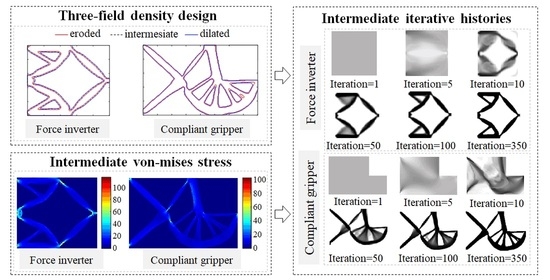
Figure 6b displays the different thresholds for the contours of the different designs, and Figure 6c–e show the contours of different designs optimized topologies for three levels of fatigue and static failure constraints. The corresponding von Mises stress distributions of the eroded, intermediate, and dilated designs are shown in Figure 6f–h, respectively. The von Mises stress is estimated to be approximately $100 \mathrm{M}\mathrm{P}\mathrm{a}$. To prevent static failure, which is also referred to as one-time loading failure, the maximum absolute value of the sum of the alternating stress and the mean stress should be less than the yield strength at the second constraint. To ensure that the force inverter satisfies this constraint, the modified Goodman fatigue criteria, $L_{i,1}$ and $L_{i,2}$, and the static failure criteria, $L_{i,3}$ and $L_{i,4}$, are employed for the three-field density projection with eroded, intermediate, and dilated projections, as shown in

Table 2. The resultant values of the force inverter.

Parameter	Symbol	Eroded	Intermediate	Dilated
Output displacement	$u_{out}$	99.8876	99.8850	99.8909
Amplification ratio	$A_r$	0.69	0.733	0.727
Volume fraction	$V$	0.252	0.302	0.346
Fatigue failure 1	$L_{i,1}$	0.84	0.89	1.26
Fatigue failure 2	$L_{i,2}$	0.678	0.75	0.865
Static failure 1	$L_{i,3}$	0.378	0.418	0.482
Static failure 2	$L_{i,4}$	0.378	0.418	0.482
Gray level indicator	$\mathrm{M}\mathrm{n}\mathrm{d}$	2.5%	1.5%	1.8%

.

To verify the results obtained from the MATLAB implementation, three different combinations were employed to evaluate the fatigue and static damage resistance of the optimal design. As illustrated in Figure 7a–c, the eroded, intermediate, and dilated designs of the Goodman fatigue criteria were tested under different conditions. In this Figure 7a–c, the color pink is utilized to represent the von Mises theory, blue is employed to signify the Sines theory, and green is used to denote the Sines von Mises theory. The outcomes demonstrate that the force inverter is capable of satisfying both the fatigue and static failure constraints, and all test conditions fall within the modified Goodman safety zone. Furthermore, it is evident that the fatigue life of the inverter is infinite when subjected to the designated load conditions during the design phase. It should be noted that the output displacement of the compliant mechanism may be reduced due to the limitations imposed via the partial constraints on fatigue and static failure for maximum output displacement. Meanwhile, the different designs for the different thresholds are displayed in Figure 8a–c.

To check the maximum output displacement of the optimal design, the deformation configurations of the obtained inverter are shown in Figure 9a–c, corresponding to the eroded, intermediate, and dilated deformation configurations of the inverter, respectively. We also presented the corresponding data for the inverter with three threshold projections, as shown in Table 2. The maximum output displacements of three threshold projection are 99.8876, 99.8850, and 99.8909, and the corresponding amplification ratios are 0.69, 0.733, and 0.727, respectively. It can be observed that the dilated value, $L_{i,1}$, is greater than 1 and is close to 1, which may be caused via numerical instability and may not affect our final design results. Meanwhile, the discreteness of the obtained design adds a gray level indicator, Mnd, measurer for gray level measurements. When every element exhibits intermediate density, or ${\overline{\tilde{\rho }}}_i=0.5$, the indicator’s value is Mnd = 100%. The indicator’s value is Mnd = 0% if all elements have densities of 0 or 1.

Finally, the convergence history of the intermediate threshold projections of the compliant inverter are depicted in Figure 10, which are the objective function and volume constraint. Note: since the displacement directions of the output end and the input end are opposite, the optimization result converges downward, and an additional 100 mm displacement is added to the objective function, which is consistent with our design philosophy.

6.2. Numerical Examples of the Gripper

The gripper presented in Figure 11a serves as the second example, with its design domain dimensions specified as $\mathrm{a}\times b=160\times 100 \mathrm{m}{\mathrm{m}}^2$. The analysis domain comprises a rectangular design domain denoted by ${\mathsf{\Omega }}_d$, and a rectangular void non-design domain labeled as ${\mathsf{\Omega }}_v$. The rectangular void non-design domain, ${\mathsf{\Omega }}_v$, has an area of $\mathrm{b}/2\times b/2=50\times 50 \mathrm{m}{\mathrm{m}}^2$. An input force of $F_{in,1}$ is applied at the input port, $O_{in,1}$, and the area, $\Gamma$, is fixed. The filter radius is set to $R=4.8 \mathrm{m}\mathrm{m}$, while the smoothness parameter is specified as $\beta =30$. The dilated design is set to ${\eta }_d=0.3$, whereas the eroded design is established at ${\eta }_e=0.7$, and the intermediate design is assigned a value of ${\eta }_i=0.5$.

The optimized topologies for different designs with respect to three levels of fatigue and static failure constraints are displayed in Figure 11c–e in terms of their corresponding contours. Moreover, Figure 11f–h depict the corresponding von Mises stress distribution of the eroded, intermediate, and dilated designs, which were found to be approximately 100 MPa. Furthermore, the modified Goodman fatigue criteria, $L_{i,1}$ and $L_{i,2}$, as well as the static failure criteria, $L_{i,3}$ and $L_{i,4}$, were employed in the three-field density projection, utilizing the eroded, intermediate, and dilated projections, as depicted in

Table 3. The resultant values of the compliant gripper.

Parameter	Symbol	Eroded	Intermediate	Dilated
Output displacement	$u_{out}$	99.9698	99.9665	99.9657
Amplification ratio	$A_r$	0.204	0.231	0.238
Volume fraction	$V$	0.266	0.307	0.327
Fatigue failure 1	$L_{i,1}$	0.697	0.786	0.817
Fatigue failure 2	$L_{i,2}$	0.587	0.663	0.689
Static failure 1	$L_{i,3}$	0.327	0.370	0.384
Static failure 2	$L_{i,4}$	0.327	0.370	0.384
Gray level indicator	$\mathrm{M}\mathrm{n}\mathrm{d}$	2.8%	0.9%	1.0%

Note: It should be noted that the lower output displacement performance is justifiable due to the robust strength-constrained approach, which faces an additional challenge in terms of strength feasibility. This challenge must be ensured for three distinct fields of relative densities, which further adds to the complexity of the problem.

. The three threshold projection maximum output displacements are 99.9698, 99.9665, and 99.9657, with corresponding amplification ratios of 0.204, 0.231, and 0.238, respectively. Both the fatigue and static failure constraints of the three-threshold projection meet the strength design requirements, ensuring an infinite lifespan of the mechanism under a given load. Furthermore, the design incorporates a gray level indicator, Mnd, for measuring gray levels discretely. The maximum gray level is 2.8%, indicating that the design achieves high precision in its gray level measurements. Furthermore, the eroded, intermediate, and dilated designs of the Goodman fatigue criteria were tested in three different combinations, as shown in Figure 12a–c.

The deformation configurations of the compliant gripper are illustrated in Figure 13a–c, which correspond to the eroded, intermediate, and dilated configurations of the inverter, respectively. Moreover, the feature size that controls the topology optimization results effectively prevents the appearance of unmanufacturable thin levers, holes, and other structures. Finally, Figure 14 depicts the convergence history of the intermediate threshold projections of the compliant gripper, which includes the objective function and volume constraint.

7. Conclusions

This study presents a novel approach for topology optimization of compliant mechanisms that addresses issues related to static strength, fatigue failure, and manufacturability. The proposed method involves converting the static strength and fatigue failure constraints into different stress constraints, which are then addressed using stress relaxation techniques and p-norm aggregation approaches in the context of continuum topology optimization. Furthermore, the introduced maximum operator approach is utilized to address non-differentiable kink issues. Considering that different pieces of machining equipment have different machining accuracies, a three-field density projection approach is employed to ensure manufacturability of the optimized design. The proposed method is implemented using an improved SIMP interpolation model, and the design problem is solved using the GCMMA algorithm based on sensitivity analysis. Finally, the effectiveness of the proposed method is demonstrated through two numerical examples:

• The von Mises stresses in the force inverter and compliant gripper were found to be approximately 120 MPa and 100 MPa, respectively. These stresses were below the material’s strength limit of 275 MPa.
• Compared with the previous topology optimization without fatigue constraints, the fatigue-constrained topology optimization can more effectively suppress the one-node hinge connection problems and avoid the phenomenon of stress concentration. Moreover, the maximum stress value of the compliant mechanism obtained using the fatigue-constrained topology optimization was lower, and the stress distribution was more uniform.
• The three-field density projection approach was successfully employed to control the minimum size in the layout optimization, thereby meeting the manufacturing process requirements. In addition, a gray level indicator, Mnd, was utilized to measure the gray level, and the maximum gray level of the real design was found to be less than 1.5%. The effectiveness of the proposed method was effectively demonstrated through two numerical examples.

References

- Wang, R.; Zhang, X. Optimal design of a planar parallel 3-dof nanopositioner with multi-objective. Mech. Mach. Theory 2017, 112, 61–83. [Google Scholar] [CrossRef]
- Alberola, J.A.M.; Fassi, I. Cyber-physical systems for micro-/nano-assembly operations: A survey. Curr. Robot. Rep. 2021, 2, 33–41. [Google Scholar] [CrossRef]
- Wang, X.; Meng, Y.; Huang, W.-W.; Li, L.; Zhu, Z.; Zhu, L. Design, modeling, and test of a normal-stressed electromagnetic actuated compliant nano-positioning stage. Mech. Syst. Signal Process. 2023, 185, 109753. [Google Scholar] [CrossRef]
- Gu, G.-Y.; Zhu, L.-M.; Su, C.-Y.; Ding, H.; Fatikow, S. Modeling and control of piezo-actuated nanopositioning stages: A survey. IEEE Trans. Autom. Sci. Eng. 2014, 13, 313–332. [Google Scholar] [CrossRef]
- Zhou, R.; Zhu, Z.-H.; Kong, L.; Yang, X.; Zhu, L.; Zhu, Z. Development of a high-performance force sensing fast tool servo. IEEE Trans. Ind. Inform. 2021, 18, 35–45. [Google Scholar] [CrossRef]
- Zhao, D.; Zhu, Z.; Huang, P.; Guo, P.; Zhu, L.; Zhu, Z. Development of a piezoelectrically actuated dual-stage fast tool servo. Mech. Syst. Signal Process. 2020, 144, 106873. [Google Scholar] [CrossRef]
- Zhao, D.; Du, H.; Wang, H.; Zhu, Z. Development of a novel fast tool servo using topology optimization. Int. J. Mech. Sci. 2023, 250, 108283. [Google Scholar] [CrossRef]
- Sano, P.; Verotti, M.; Bosetti, P.; Belfiore, N.P. Kinematic synthesis of a d-drive mems device with rigid-body replacement method. J. Mech. Des. 2018, 140, 075001. [Google Scholar] [CrossRef]
- Yeon, A.; Yeo, H.G.; Roh, Y.; Kim, K.; Seo, H.-S.; Choi, H. A piezoelectric micro-electro-mechanical system vector sensor with a mushroom-shaped proof mass for a dipole beam pattern. Sens. Actuators A Phys. 2021, 332, 113129. [Google Scholar] [CrossRef]
- Salinić, S.; Nikolić, A. A new pseudo-rigid-body model approach for modeling the quasi-static response of planar flexure-hinge mechanisms. Mech. Mach. Theory 2018, 124, 150–161. [Google Scholar] [CrossRef]
- Kenton, B.J.; Leang, K.K. Design and control of a three-axis serial-kinematic high-bandwidth nanopositioner. IEEE/ASME Trans. Mechatron. 2011, 17, 356–369. [Google Scholar] [CrossRef]
- Ryu, J.W.; Lee, S.-Q.; Gweon, D.-G.; Moon, K.S. Inverse kinematic modeling of a coupled flexure hinge mechanism. Mechatronics 1999, 9, 657–674. [Google Scholar] [CrossRef]
- Ling, M.; Cao, J.; Zeng, M.; Lin, J.; Inman, D.J. Enhanced mathematical modeling of the displacement amplification ratio for piezoelectric compliant mechanisms. Smart Mater. Struct. 2016, 25, 075022. [Google Scholar] [CrossRef]
- Li, C.; Chen, S.-C. Design of compliant mechanisms based on compliant building elements. Part I: Principles. Precis. Eng. 2023, 81, 207–220. [Google Scholar] [CrossRef]
- Chen, F.; Dong, W.; Yang, M.; Sun, L.; Du, Z. A pzt actuated 6-dof positioning system for space optics alignment. IEEE/ASME Trans. Mechatron. 2019, 24, 2827–2838. [Google Scholar] [CrossRef]
- Zhu, Z.; Zhou, X.; Liu, Z.; Wang, R.; Zhu, L. Development of a piezoelectrically actuated two-degree-of-freedom fast tool servo with decoupled motions for micro-/nanomachining. Precis. Eng. 2014, 38, 809–820. [Google Scholar] [CrossRef]
- Zhu, B.; Chen, Q.; Jin, M.; Zhang, X. Design of fully decoupled compliant mechanisms with multiple degrees of freedom using topology optimization. Mech. Mach. Theory 2018, 126, 413–428. [Google Scholar] [CrossRef]
- Lum, G.Z.; Teo, T.J.; Yeo, S.H.; Yang, G.; Sitti, M. Structural optimization for flexure-based parallel mechanisms-towards achieving optimal dynamic and stiffness properties. Precis. Eng. 2015, 42, 195–207. [Google Scholar] [CrossRef]
- Jin, M.; Zhang, X. A new topology optimization method for planar compliant parallel mechanisms. Mech. Mach. Theory 2016, 95, 42–58. [Google Scholar] [CrossRef]
- Pinskier, J.; Shirinzadeh, B.; Ghafarian, M.; Das, T.K.; Al-Jodah, A.; Nowell, R. Topology optimization of stiffness constrained flexure-hinges for precision and range maximization. Mech. Mach. Theory 2020, 150, 103874. [Google Scholar] [CrossRef]
- Pham, M.T.; Yeo, S.H.; Teo, T.J.; Wang, P.; Nai, M.L.S. A decoupled 6-dof compliant parallel mechanism with optimized dynamic characteristics using cellular structure. Machines 2021, 9, 5. [Google Scholar] [CrossRef]
- Zhu, B.; Zhang, X.; Zhang, H.; Liang, J.; Zang, H.; Li, H.; Wang, R. Design of compliant mechanisms using continuum topology optimization: A review. Mech. Mach. Theory 2020, 143, 103622. [Google Scholar] [CrossRef]
- Liu, M.; Zhan, J.; Zhu, B.; Zhang, X. Topology optimization of flexure hinges with a prescribed compliance matrix based on the adaptive spring model and stress constraint. Precis. Eng. 2021, 72, 397–408. [Google Scholar] [CrossRef]
- Liu, C.-H.; Chen, Y.; Yang, S.-Y. Topology optimization and prototype of a multimaterial-like compliant finger by varying the infill density in 3d printing. Soft Robot. 2022, 9, 837–849. [Google Scholar] [CrossRef] [PubMed]
- Dorn, W.S. Automatic design of optimal structures. J. Mec. 1964, 3, 25–52. [Google Scholar]
- Nishiwaki, S.; Frecker, M.I.; Min, S.; Kikuchi, N. Topology optimization of compliant mechanisms using the homogenization method. Int. J. Numer. Methods Eng. 1998, 42, 535–559. [Google Scholar] [CrossRef]
- Takezawa, A.; Nishiwaki, S.; Kitamura, M. Shape and topology optimization based on the phase field method and sensitivity analysis. J. Comput. Phys. 2010, 229, 2697–2718. [Google Scholar] [CrossRef]
- Wang, N.F.; Zhang, X.M. Topology optimization of compliant mechanisms using pairs of curves. Eng. Optim. 2015, 47, 1497–1522. [Google Scholar] [CrossRef]
- Ansola, R.; Veguería, E.; Canales, J.; T’arrago, J.A. A simple evolutionary topology optimization procedure for compliant mechanism design. Finite Elem. Anal. Des. 2007, 44, 53–62. [Google Scholar] [CrossRef]
- Luo, Z.; Tong, L.; Wang, M.Y.; Wang, S. Shape and topology optimization of compliant mechanisms using a parameterization level set method. J. Comput. Phys. 2007, 227, 680–705. [Google Scholar] [CrossRef]
- Wang, R.; Zhang, X.; Zhu, B. Imposing minimum length scale in moving morphable component (mmc)-based topology optimization using an effective connection status (ecs) control method. Comput. Methods Appl. Mech. Eng. 2019, 351, 667–693. [Google Scholar] [CrossRef]
- Luo, Z.; Chen, L.; Yang, J.; Zhang, Y.; Abdel-Malek, K. Compliant mechanism design using multi-objective topology optimization scheme of continuum structures. Struct. Multidiscip. Optim. 2005, 30, 142–154. [Google Scholar] [CrossRef]
- Duysinx, P.; Bendsøe, M.P. Topology optimization of continuum structures with local stress constraints. Int. J. Numer. Methods Eng. 1998, 43, 1453–1478. [Google Scholar] [CrossRef]
- de Troya, M.A.S.; Tortorelli, D.A. Adaptive mesh refinement in stress-constrained topology optimization. Struct. Multidiscip. Optim. 2018, 58, 2369–2386. [Google Scholar] [CrossRef]
- Chu, S.; Gao, L.; Xiao, M.; Luo, Z.; Li, H. Stress-based multi-material topology optimization of compliant mechanisms. Int. J. Numer. Methods Eng. 2018, 113, 1021–1044. [Google Scholar] [CrossRef]
- de Assis Pereira, A.; Cardoso, E.L. On the influence of local and global stress constraint and filtering radius on the design of hinge-free compliant mechanisms. Struct. Multidiscip. Optim. 2018, 58, 641–655. [Google Scholar] [CrossRef]
- Conlan-Smith, C.; James, K.A. A stress-based topology optimization method for heterogeneous structures. Struct. Multidiscip. Optim. 2019, 60, 167–183. [Google Scholar] [CrossRef]
- Deng, H.; Vulimiri, P.S.; To, A.C. An efficient 146-line 3d sensitivity analysis code of stress-based topology optimization written in matlab. Optim. Eng. 2021, 23, 1733–1757. [Google Scholar] [CrossRef]
- Roin, T.; Montemurro, M.; Pailh, J. Stress-based topology optimization through non-uniform rational basis spline hyper-surfaces. Mech. Adv. Mater. Struct. 2022, 29, 3387–3407. [Google Scholar] [CrossRef]
- Bruggi, M. On an alternative approach to stress constraints relaxation in topology optimization. Struct. Multidiscip. Optim. 2008, 36, 125–141. [Google Scholar] [CrossRef]
- Le, C.; Norato, J.; Bruns, T.; Ha, C.; Tortorelli, D. Stress-based topology optimization for continua. Struct. Multidiscip. Optim. 2010, 41, 605–620. [Google Scholar] [CrossRef]
- Jeong, S.H.; Choi, D.-H.; Yoon, G.H. Fatigue and static failure considerations using a topology optimization method. Appl. Math. Model. 2015, 39, 1137–1162. [Google Scholar] [CrossRef]
- Nabaki, K.; Shen, J.; Huang, X. Evolutionary topology optimization of continuum structures considering fatigue failure. Mater. Des. 2019, 166, 107586. [Google Scholar] [CrossRef]
- Holmberg, E.; Torstenfelt, B.; Klarbring, A. Fatigue constrained topology optimization. Struct. Multidiscip. Optim. 2014, 50, 207–219. [Google Scholar] [CrossRef]
- Collet, M.; Bruggi, M.; Duysinx, P. Topology optimization for minimum weight with compliance and simplified nominalstress constraints for fatigue resistance. Struct. Multidiscip. Optim. 2017, 55, 839–855. [Google Scholar] [CrossRef]
- Oest, J.; Lund, E. Topology optimization with finite-life fatigue constraints. Struct. Multidiscip. Optim. 2017, 56, 1045–1059. [Google Scholar] [CrossRef]
- Chen, Z.; Long, K.; Wen, P.; Nouman, S. Fatigue-resistance topology optimization of continuum structure by penalizing the cumulative fatigue damage. Adv. Eng. Softw. 2020, 150, 102924. [Google Scholar] [CrossRef]
- Sigmund, O. Manufacturing tolerant topology optimization. Acta Mech. Sin. 2009, 25, 227–239. [Google Scholar] [CrossRef]
- Wang, F.; Jensen, J.S.; Sigmund, O. Robust topology optimization of photonic crystal waveguides with tailored dispersion properties. JOSA B 2011, 28, 387–397. [Google Scholar] [CrossRef]
- Schevenels, M.; Lazarov, B.S.; Sigmund, O. Robust topology optimization accounting for spatially varying manufacturing errors. Comput. Methods Appl. Mech. Eng. 2011, 200, 3613–3627. [Google Scholar] [CrossRef]
- Lazarov, B.S.; Schevenels, M.; Sigmund, O. Robust design of large-displacement compliant mechanisms. Mech. Sci. 2011, 2, 175–182. [Google Scholar] [CrossRef]
- Guo, X.; Zhang, W.; Zhang, L. Robust structural topology optimization considering boundary uncertainties. Comput. Methods Appl. Mech. Eng. 2013, 253, 356–368. [Google Scholar] [CrossRef]
- Zhang, W.; Kang, Z. Robust shape and topology optimization considering geometric uncertainties with stochastic level set perturbation. Int. J. Numer. Methods Eng. 2017, 110, 31–56. [Google Scholar] [CrossRef]
- da Silva, G.A.; Beck, A.T.; Sigmund, O. Topology optimization of compliant mechanisms with stress constraints and manufacturing error robustness. Comput. Methods Appl. Mech. Eng. 2019, 354, 397–421. [Google Scholar] [CrossRef]
- da Silva, G.A.; Beck, A.T.; Sigmund, O. Topology optimization of compliant mechanisms considering stress constraints, manufacturing uncertainty and geometric nonlinearity. Comput. Methods Appl. Mech. Eng. 2020, 365, 112972. [Google Scholar] [CrossRef]
- Liu, M.; Zhan, J.; Zhu, B.; Zhang, X. Topology optimization of compliant mechanism considering actual output displacement using adaptive output spring stiffness. Mech. Mach. Theory 2020, 146, 103728. [Google Scholar] [CrossRef]
- Svanberg, K. Mma and Gcmma-Two Methods for Nonlinear Optimization; KTH: Stockholm, Sweden, 2007; Volume 1, pp. 1–15. [Google Scholar]
- Wang, F.; Lazarov, B.S.; Sigmund, O. On projection methods, convergence and robust formulations in topology optimization. Struct. Multidiscip. Optim. 2011, 43, 767–784. [Google Scholar] [CrossRef]
- Qian, X.; Sigmund, O. Topological design of electromechanical actuators with robustness toward over-and under-etching. Comput. Methods Appl. Mech. Eng. 2013, 253, 237–251. [Google Scholar] [CrossRef]
Figure 1.
Synthesis of compliant mechanisms.
Figure 2.
One cycle of the history in high cycle fatigue approach: (a) one-cycle constant and proportional loading history, and (b) one-cycle stress history.
Figure 3.
Modified Goodman diagram fatigue criterion: (a) modified Goodman diagram; the static failure envelopes of the present optimization problem (b) and (c).
Figure 4.
Normalized length scale on the intermediate design as function of the threshold a for the robust formulation: (a) versus curve useful for design, and (b) the η versus b/R curve useful for design.
Figure 5.
A flowchart of the topology optimization of compliant mechanism optimization algorithm.
Figure 6.
The force inverter. (a) The design domain; (b) the contours of different designs: eroded , intermediate , and dilated ; optimized topologies for three levels of fatigue constraints (c) eroded designs, (d) intermediate designs, and (e) dilated designs; the von Mises stress distribution of (f) eroded, (g) intermediate, and (h) dilated designs.
Figure 7.
The eroded, intermediate, and dilated designs of the Goodman fatigue criteria of force inverter: (a) the eroded , (b) intermediate , and (c) dilated designs of the threshold projection filters.
Figure 8.
The threshold projection filters of force inverter: (a) the eroded , (b) intermediate , and (c) dilated designs of the threshold projection filters.
Figure 9.
Deformation configuration of force inverter, (a) the eroded , (b) intermediate , and (c) dilated .
Figure 10.
Optimization history for the force inverter.
Figure 11.
The compliant gripper. (a) The design domain; (b) the contours of different designs: eroded , intermediate , and dilated ; optimized topologies for three levels of fatigue constraints: (c) eroded designs, (d) intermediate designs, and (e) dilated designs; the von Mises stress distribution of (f) eroded, (g) intermediate, and (h) dilated designs.
Figure 12.
The eroded, intermediate, and dilated designs of the Goodman fatigue criteria of compliant gripper: (a) the eroded , (b) intermediate , and (c) dilated designs of the threshold projection filters.
Figure 13.
Deformation configurations of compliant gripper: (a) eroded , (b) intermediate , and (c) dilated .
Figure 14.
Optimization history for the compliant gripper.