1. Introduction
In daily life, especially in the study of natural science, some phenomena are often monitored and evaluated in order to formulate plans and programs. The data collected from these activities are often presented in the form of a time series. In analyzing and predicting time series data, in addition to traditional mathematical or physical models, the most common approach is to use artificial intelligence modeling, such as deep learning, for analysis and prediction. The technique of deep learning has been well developed in the past decade, and the technology has gradually matured; e.g., artificial neural network (ANN), recurrent neural network (RNN), long short-term memory artificial neural network (LSTM), convolutional neural network (CNN), etc. have been popularized and used in many new fields and applications. The requirements of today’s information systems are very time sensitive and adaptive, such as tracking and analyzing real-time data. If the processes and time required for the analysis of time series data can be effectively shortened, the usability and timeliness of these data products will be greatly improved, making them much easier and more willing to be used and accepted by the users.
This study will propose a new approach called the MTS decomposition and recombining model (which will be referred to as the MTS-DR model in the remaining sections of this article). Even if there are some enhanced algorithms and hardware methods for parallel computing, a certain number of epochs are usually required to obtain the ideal training results and make the loss curve flat and stable. This is because there are many details hidden in the MTS dataset. However, as is known, any MTS must contain a portion of the seasonal or cyclic oscillation [
1]. Especially for those daily events in nature, many periodic and cyclical features can be collected from time to time. Therefore, if those cyclical time series data are decomposed into small portions of waves, the seasonal portions must form a very stable phase oscillation over a certain period of time in an MTS. Then, this will be a redundant procedure for these seasonal waves to be trained. After this kind of seasonal portion of the MTS model is trained, the test set is obtained, and the actual curve will inevitably overlap with the predictive curve.
The purpose of this study aims to point out that when predicting MTS, e.g., the air quality of small urban cities, as MTS has its own very different characteristics, the MTS analysis in advance is helpful for the construction of the model and the improvement in efficiency. For this reason, using some statistical techniques and tools to analyze and decompose MTS and then model it, significant improvements in performance and efficiency can be achieved. This research attempts to use the decomposed wave components of the original time series to model and train them one by one independently to predict the future situation and then recombine them. By comparing the predictions with the original model, it is found that both the running time and the prediction accuracy have improved significantly. On the other hand, by using some statistical and mathematical methods, an obvious 24 h oscillation is found in the time series of concentrations of each type of air pollutant element. The study also showed that, through visualization of the final forecast results, the MTS-DR model was mostly reliable and ideal for predicting each trend shifting point. The research results show that the running time and accuracy of ANN-type model forecasting time series can be improved without adding additional operating resources and data sources, i.e., at zero cost. These results can be applied to real-time artificial intelligence systems for monitoring and predicting changes in any time series that contains oscillation and seasonality.
In order to make the novelty not limited to a certain kind of data, in this study, the method is applied to the datasets of six air pollutants with different characteristics, such as: PM, ozone, sulfur dioxide, nitrogen dioxide, and carbon monoxide, all in the physical, chemical, interaction with elements of the natural environment, and periodicity, which behave very differently. Therefore, this method has a certain degree of commonality and can be applied to other types of datasets, especially those with obvious seasonality that are easily affected by other external factors.
2. Materials and Methods
The goal of this study is to find a way to increase the accuracy and lower the training time of a deep learning model so that it can be re-trained from time to time and adopted as a core part of a real-time prediction system. Therefore, the experiments for proving this concept are to build a multivariate LSTM model to predict the air quality in Macau by using a certain number of weather elements and the concentrations of the air pollutants themselves. The issue of air pollution and improvement policies are the main concerns of many advanced cities in the world today, including Macao. Concentrations of air pollutants can have adverse effects on public health and the environment. Therefore, accurate forecasting of air quality is important to help policymakers take the necessary precautions and reduce exposure to harmful pollutants. The tools used for experiments in research include Anaconda, Python, PyTorch, NetCDF, MatLAB, and those related software libraries and packages.
There are many methods to predict the time series data, e.g., regression, auto-regression integrated moving average ARIMA, wavelet analysis, mathematical and physical models, and machine learning. To predict the time series of air quality, the concentrations of the air pollutants need to be monitored, and then the air quality can be determined. As the dispersion of the concentrations of air pollutants is affected and conveyed by the atmospheric events, e.g., the weather, rain, strong wind, etc. Therefore, when monitoring and forecasting air quality, it is necessary to process and analyze weather conditions and air pollutant concentrations at the same time. In the frontier work of researching and predicting air quality, introducing a variety of meteorological features into the model, such as air temperature, dew point, wind speed, wind direction, cloud cover, water vapor pressure, visibility, etc., has been widely used to predict the concentration levels of PM
2.5, PM
10, SO
2, NO
2, ozone, and CO. This is because multivariate models that include multiple weather elements perform better with higher accuracy [
2]. The synergistic effect of various air pollutants and weather affecting human health, i.e., the relationship between weather conditions, air pollution, and human health. That study found that for certain types of air pollution, the impact on human health varies under specific weather conditions, and that pollutant interactions significantly affect this relationship [
3]. Multivariate deep learning is a good alternative and appropriate to solve this kind of problem. In addition to analyzing local air pollutants, meteorological and long-range circulation patterns also affect the distribution of seasonal and daily concentrations, e.g., clean air masses from the Atlantic Ocean and mild temperatures throughout the year lead to relatively low concentrations with very large daily and seasonal variations [
4].
2.1. MTS Analysis
As mentioned in the previous section, when forecasting some time series, the model needs multivariate time series (MTS) to improve its accuracy. There are some common characteristics of multivariate time series (MTS). It is called multivariate; that is, MTS involves multiple interdependent and mutually influencing variables. It should be non-stationary, which means the statistical properties of MTS change over time, making it difficult to predict future values, but there is still a developing trend. It is highly dimensional, and MTS can have a large number of variables, making analysis and modeling challenging. Dependencies between variables in MTS can be complicated and non-linear. In addition to an overall development trend, MTS also has a rather obvious seasonality. Therefore, seasonal patterns should be considered and taken into an account when modeling forecast. Some techniques, such as wavelet analysis, Fourier analysis, frequency domain, auto-correlation, and partial auto-correlation, can be used to identify the different levels of oscillation and seasonality.
The decomposition of a time series into its component parts is a set of a mathematical processes. Studies have shown that the introduction of wavelet analysis in modeling components will effectively improve the quality of predictions under different weather characteristics, for example, wavelet functions. Generally speaking, a typical time series of geophysical elements consists of two or more components: Trend components and details; they must have a definite periodic oscillation and contain chaotic details without any regularity [
5]. Data decomposition can better identify the characteristics of time series data in the training phase; e.g., splitting the daily time series into different parts can improve the ability to express information and make the characteristics of the sequence clear. The description makes the model have better nonlinear fitting ability [
6]. The simplest and most common method is often used to identify trends, seasonal patterns, and other potential factors that may affect the data. The most common method for time series decomposition is the additive model, which uses the following Equation (1):
where
Y(
t) is the observations,
T(
t) is the trend component,
S(
t) is the seasonal component,
C(
t) is the periodic component, and
I(
t) is the irregular or random component.
Each of these components can be further broken down into their own components. For example,
T(
t) can be decomposed into linear and nonlinear components. The decomposition process can also be done using multiplicative models or other methods such as Fourier analysis or wavelet analysis. In addition, there are some other advanced methods used in different fields and applications to analyze and decompose a time series, such as wavelet analysis and Fourier analysis. The Fourier analysis formula is Equation (2), as follows:
where
A0 is the average value of the time series,
Ai and
Bi are the Fourier coefficients, and
fi is the frequency of the signal. The common formula to express both Fourier analysis and wavelet analysis is Equation (3), as follows:
From the above, the seasonal part of a Fourier analysis formula is the sine and cosine terms that are used to model periodic patterns in a time series. These terms are used to capture the cyclical nature of the data, such as seasonal effects, and can be used to forecast future values. In multivariate modeling, a collection of multiple time series is treated as a unified entity. Decomposing the univariate time series into a series of distinct frequency components via discrete Fourier transform (DFT) improves deep neural architectures within LSTM models and deep stacks of fully connected layers [
7]. Some studies decompose the high variability time series into several sub-sequences with lower variability in wavelet analysis and apply forecasting strategies to each sub-sequence at different scales. In this way, the prediction problem can be decomposed into several simpler tasks, thus improving the prediction accuracy [
8]. Since the seasonal part of a wavelet analysis formula is the part that captures the periodic fluctuations in the data, it is usually represented by a single or a simple combination of sinusoidal functions with a period equal to the length of the season.
There are some research methods that decompose time series of meteorological and air pollutant data into long-term and short-term components; e.g., there is a chance that there is a low correlation between the ozone’s short-term component and solar radiation. This is used to filter time series by analyzing different components and different correlation structures and correlations in terms of time duration [
9]. Some studies on how to use frequency information to improve the efficiency of time series forecasting are using frequency-domain analysis of seasonal anomalies and contrast spectral information to explore time-frequency consistency. Since the basic functions of the Fourier transform are fixed (such as trigonometric functions), the extracted frequency features are domain invariant. These features are insensitive to unexpected noise changes, and due to this limitation, there have been few models that combine Fourier analysis with the learning ability of neural networks [
10]. Some research results show that if the instability of the original data can be successfully reduced and the inherent complexity of the AQI data can be simplified, such as using the (complete ensemble empirical mode decomposition with adaptive noise-variational mode decomposition-general regression neural network) CEEMDAN-VMD-GRNN model, it can be used as an effective method for predicting highly unstable and complex data. Time series decomposition is also applied in that study [
11].
2.2. Auto-correlation of the TS
Auto-correlation, as the name suggests, is a mathematical representation of the degree of similarity between a given time series and its lagged version of itself in continuous time intervals. It is conceptually similar to the correlation between two different time series, but it uses the different versions of time slices of the same time series for both, i.e., one in the original form and the other in the version lagged by one or more units of time periods. In other words, it measures the relationship between the current value of a variable and its past values. An auto-correlation of “+1” indicates a perfect positive correlation, while “−1” indicates a perfect negative correlation. In real-world applications, e.g., auto-correlation can be used to measure how much the past price of a product affects its future price, etc. In
Figure 1, for this research, the auto-correlation of each time series is used to visualize and explore its 24 h oscillation and seasonality. It can be seen that there are sine waves repeating at 24 h, 48 h positions, etc., in the small graphs of PM
2.5, PM
10, SO
2, NO
2, ozone, CO, air temperature, and water vapor pressure deficit (VPD), respectively, with the auto-correlation visualization. In particular situations, it is important to note that these obvious patterns may not exist throughout the whole time series because there may be some anomalies or outliers caused by severe weather, special atmospheric phenomena, or human activities that affect the diffusion or dispersion of the air pollutants.
2.3. Design and Building of the Multivariate Model
The focus of this study is to explore the feasibility of the proposed MTS-DR and find that it is feasible. Initially, we wanted to use the most common LSTM, which is the most commonly used ANN type for time series prediction. This is to shorten the research time of this phase, as it is planned to integrate these results into a larger project and publish more in-depth applied research articles.
In this study, a typical type of deep learning model is first chosen. Because of the balanced performance and efficiency, a multivariate LSTM model will be constructed to predict the air quality in Macao, which is a city located in the sub-tropical region, as LSTM is a kind of typical and balanced ANN-type model. Multivariate models have been widely used due to higher accuracy, i.e., with the same ANN-type model, as the number of input variables increases, the predicted mean absolute error MAE and mean squared error MSE gradually decrease, which means that adding multivariate models can help to improve the prediction accuracy of the concentration of air pollutants [
12]. The method used also includes the use of historical data from different sources, such as Macao Meteorological Stations and Air Quality Monitoring Stations. Before being used to train the model, the data will be pre-processed and cleaned, such as by removing NAN and outliers, etc. We will use a multivariate LSTM model that takes in various weather factors such as temperature, humidity, wind speed, and the concentration of air pollutants such as PM
2.5, PM
10, NO
2, SO
2, etc.
When considering ANN-type neural network model modeling, in general, LSTM models are more stable than RNN and GRU models, and they are much easier to build. Sometimes CNNLSTM gives the smallest error [
13], but not often. In a study, the MLP, RNN, and LSTM models have been compared for predicting air pollutants such as PM
10 and SO
2, and LSTM performs better, and LSTM estimates PM
10 and SO
2 air pollutants are closer to the true value [
14]. Thus, by synthesizing the above, it will be much easier and more convenient to use a less resource-based ANN-type model, LSTM. The architecture of a multivariate LSTM model will consist of multiple layers of LSTM cells, followed by fully connected layers for prediction. The input layer will contain various features such as temperature, humidity, wind speed, and the concentration of the air pollutant itself. The output layer will predict the concentration of each pollutant for the next time step.
2.4. MTS Data Preparation and Acquisition
The MTS models (including the old, MTS-DR, ARIMA) will include the year 2019 hourly data of these meteorological elements: Air temperature, humidity, dew point temperature, water vapor deficit, precipitation, u-vector and v-vector of wind, wind direction, wind speed, wind gust, and boundary layer height of 5 locations in Macao. The design of a multivariate LSTM model will include the following steps. The first is data collection. To consider the availability and feasibility, Macao, as a small urban city, is chosen because there is a good monitoring network for the six common air pollutants. The reanalysis data from ECMWF is very reliable and open to use for academic and research purposes. Thus, the data from the above two sources, i.e., the local auto-weather stations and air quality monitoring stations, as well as some reanalysis data, were obtained from the local weather forecast institution and ECMWF data, respectively, through the Internet. This information is regularly released to the public [
15,
16,
17]. Next, the data will be pre-processed and cleaned before being used to train the model, stored in big data chunks, and partitioned by year with the NetCDF library.
A multivariate LSTM model will then be designed with multiple layers of LSTM cells, followed by fully connected layers for prediction. As mentioned in the previous section, in order to conduct experiments to demonstrate the concepts introduced in this study, a multivariate ANN-type model was considered and designed. Some studies have proved that decomposed time series models are more accurate, which means that various algorithms are more efficient in analyzing nonlinear and non-stationary time series by decomposing time series [
18]. After balancing factors such as feasibility, availability, efficiency, and effectiveness, LSTM was adopted for the proposed MTS-DR model. On the other hand, many studies have shown that the LSTM network with long short-term memory function in hidden neurons can effectively and conveniently predict air quality, make model training more perfect, and better avoid errors. Therefore, an LSTM framework ANN with 2 hidden layers, totaling 4 layers of neurons and 50 multivariate inputs, was designed and constructed. All experiments are run on this model. When defining the number of nodes in the hidden layer, after comparing different test results, from the initial 16 nodes to the final version of 256 nodes. Each experiment will use the learning rate and number of epochs to run as determined above. The activation function is ReLU(). The pollutant concentration should be positive, regardless of observation or prediction. However, it is strongly recommended that the usual sigmoid and tanh for LSTM be adopted when used in other kinds of data. In general, it has had very little impact on this study. Since the pollutant concentration is always positive, it is hoped that the network can flexibly consider nonlinearity while approximating a linear function. The StandardScaler and MinMaxScaler functions of Python version 3.7 with SciKitLearn version 1.4 which is a free and open-source machine learning library. Preprocessing is used to standardize and preprocess the pollutant concentration time series data to a value between 0 and 1. However, after the prediction is completed, the result value is denormalized back to its original range. As shown in
Figure 2, the original time series is decomposed into three components, namely the trend, seasonal, and residual. Then, the subsets of the dataset are used as input for the sub-models for trend and residual components, while there is only a direct pipe for the seasonal components because it is not needed to predict a TS with an MSE equal to zero. The predicted trend and residual data are recombined by addition calculation with the seasonal components. In the following section, it will show the model training processes of the original dataset, trend, seasonal, and residual datasets, and the performance of the model in predicting different air pollutant concentrations.
2.5. MTS Dataset, Decomposing Module and Recombining Module
Modeling based on the decomposition of time series data and feature optimization can effectively improve the accuracy of medium- and long-range time series forecasts related to flux-behaved elements [
19]. For the decomposing module, the original multivariate time series (MTS) dataset used to predict the concentration of the six air pollutants is decomposed by the additive method into 3 components: trend (
T), seasonal (
S), and residual (
R), respectively, with the additive method of the Python TSA stats model package in Equation (4), as follows:
For the recombining module, after each sub-dataset was input into the corresponding sub-model for training, the prediction results were obtained. With the same principle of Equation (4), i.e., the summation of the 3 components of trend (T), seasonal (S), and residual (R), then derived into the original time series prediction values that are desired.
In which, the trend component is the overall level of the gradual development direction in the time series, the seasonal component is the repeated shape, and finally, the rest is the residual (see
Figure 3).
These 3 components are used to build different sub-models. Those results from the sub-models are then recombined by mathematical addition to form the final result. This main portion of the experiment is the comparison of the predicted results of the original dataset with those of the proposed MTS-DR model.
The dataset is divided into a training set and a test set according to the conventional ratio of 8:2. The model will be trained on the training set data using the backpropagation through time algorithm. The trained model will be validated on the same set of separate test set validation data to check its accuracy and error loss with mean squared error (MSE).
In the hyperparameter tuning, some hyperparameters, such as learning rate, number of epochs and layers, and neurons in each layer, are being tuned to optimize the performance of the model.
2.6. Defining the Hyperparameter Domain for Tuning
In order to analyze, synthesize, and compare scientifically, some mathematical analysis, as shown in the figures, can help to obtain a standardized and normalized environment, which is necessary for all the experiments to take place. To define the hyperparameter domain for tuning and standardizing the experiment environment, it includes defining the fixed learning rate from 0.01 to 0.0001 and selecting the number of epochs from 200 to 2000. Then, some tests were carried out under this domain, and we selected those with a small MSE. In
Figure 4a, all the trend, residual, and original TS will be best trained with a learning rate of 0.01. Thus, for all the experiments that would take place, the learning rate would be fixed at 0.01. After standardizing the learning rate, it is time for the number of epochs in each iteration to be considered. In
Figure 4b, the big yellow box shows the domain of the hyperparameter, and, with the fixed learning rate of 0.01, it is considered to be good when the mean squared error (MSE) reaches a certain level, and in this case, the MSE value of 0.000549 is calculated as the 30% C.I. reference base to the worst-case MSE result of 0.00183. With this minimum number of epochs, the result can be yielded below this yellow dotted line, so that they are defined and selected, i.e. the hyperparameters pointed by the yellow arrows in the
Figure 4b. The values of hyperparameters can be selected inside the orange, green and blue shaded portions for Trend, Residual and Original components respectively. Eventually, the number of epochs equaling 200 is selected for the trend component, 500 is selected for the residual component, and 1000 and 2000 are selected for the original TS.
2.7. Model Training
As mentioned before, the models are being trained, i.e., the old original model with the whole MTS and the model of the three components of the decomposed MTS, namely trend, seasonal, and residual, by using the Python time series analysis TSA statsmodels (see
Figure 3). The TSA statsmodels module was originally written by Jonathan Taylor and had been part of the SciPy package but was removed. During the period of Google Summer of Code 2009, this statsmodels module was amended for improvement and released as a new package. The statsmodels development team has continued to add new models, plotting tools, and statistical methods [
20]. The training time for each iteration was recorded. For the new proposed MTS-DR model, the total training time is Equation (5):
where
t is the running time and
k is the index of the sub-model for different wavelet components. In this case, there are only 3 components decomposed, i.e., trend (
T), seasonal (
S), and residual (
R). Therefore, as in Equations (6) and (7):
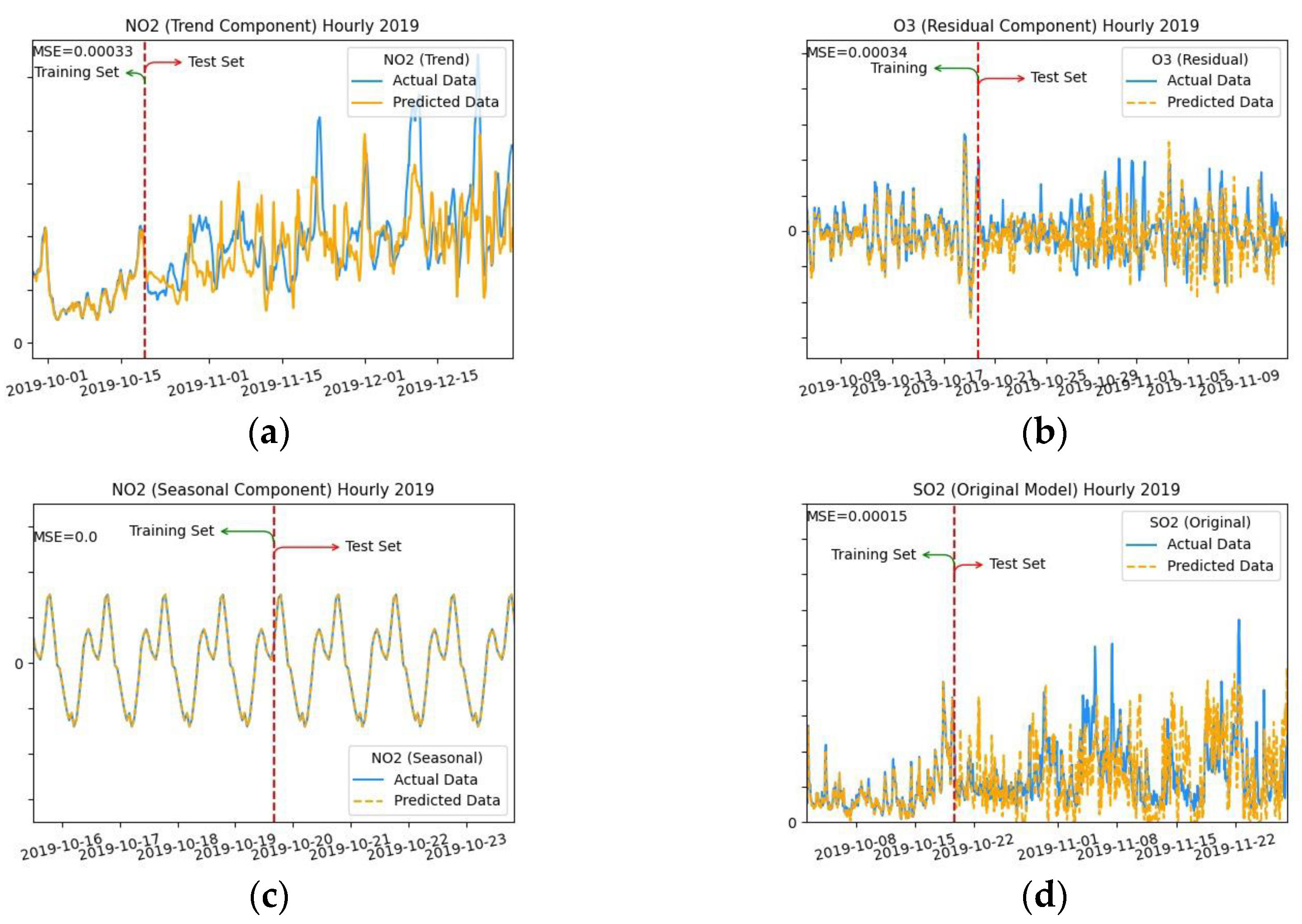
Figure 5 shows the training processes, while
Figure 5a–c shows the training processes of the proposed MTS-DR model that is expected to be able to speed up the training process, with the 3 components trained, respectively, i.e., trend, residual, and seasonal. As shown in
Figure 5c, the seasonal TS component is not necessary to be trained in the following works because the seasonal component is a very regularly repeating wave that consists of very stable cyclic phases. Thus, the predicted wave will totally overlap with the actual wave.
Figure 5d shows the training processes of the old model with the original TS.
2.8. ARIMA as Baseline Method for Evaluation
For a more objective assessment, an evaluation baseline is required. Therefore, the most popular forecasting method, auto-regression integrated moving average ARIMA, was selected and implemented on the same sets of MTS. There is a comparison of baseline methods (in this case, ARIMA) to make the evaluation clearer. To train the ARIMA model, the auto-arima function from the standard Python package called “pmdarima” is used. The whole dataset is divided into a training set and a test set with the same ratio of 8 to 2 as the MTS-DR model. After feeding the ARIMA model with all the same MTS as the input LSTM model, it is trained without fixing any parameters of the auto-arima function so that it can search for the most suitable settings by itself. Finally, use the trained ARIMA to predict the test set data. All predictions are plotted (see
Figure 6). As shown in
Figure 6, the forecast curve hovers around a certain value with only slight variations. ARIMA forecasts do not appear to be able to alert to critical changes with peak values in air pollutant concentrations. The mean absolute error MAE, median percentage absolute error MdPAE, and area under curve of accuracy probability AUC are then calculated. Since the curve predicted by ARIMA is very flat, the resulting error level is very close to that of the LSTM models. However, it is evident from
Figure 6 that the LSTM model is better at predicting key changes in air pollutant concentrations many times. This is very important for adaptive public alerting services. On the other hand, ARIMA takes a very long time to train compared to LSTM models. Longer training times are definitely a disadvantage for real-time LSTM models that rely on adaptive feature engineering (see
Table 1).
3. Results
An ideal training process for an ANN-type model is that the curve of the predicted data fits well with the curve of the actual data in the training set. If these two curves do not fit well in some cases, one of the solutions is to increase the number of epochs to allow the model to learn better. However, those experiments performed in this study were well trained, i.e., the two sets of curves overlapped well. For example, in
Figure 5, where the model stopped training, it is marked with a red dotted line. In each small graph, the left side of the red dotted line marked by the green arrow is the training set, and in this part, the yellow curve and the blue curve almost coincide, which means that the model has been trained well enough. In addition, the test set is shown on the right with the red arrow annotation, which means that the model will start making predictions here, and the yellow curve is the future value of the data predicted. Of course, the yellow and blue curves will not always overlap well here on this right-hand side portion because the prediction accuracy of any model will not be 100%.
Results of the Proposed MTS-DR Model
Figure 7 shows all the test results of prediction for the concentration of those six air pollutants by the proposed MTS-DR model after training and predicting MTS, which is decomposed by the additive method. Thus, as Equation (8)
In the above Equation (8), where trend (T), seasonal (S), and residual (R).
Then, the orange color curves show the final predicted curves of the time series; here are those 6 air pollutant elements.
Figure 7 shows the recombined trained TS of PM
2.5, PM
10, SO
2, NO
2, O
3, and CO, respectively. The orange color curves are the recombined TS, while the bold black curves are the regularly repeating seasonal, the lower black curves are the residual, and the upper black curves are the trend.
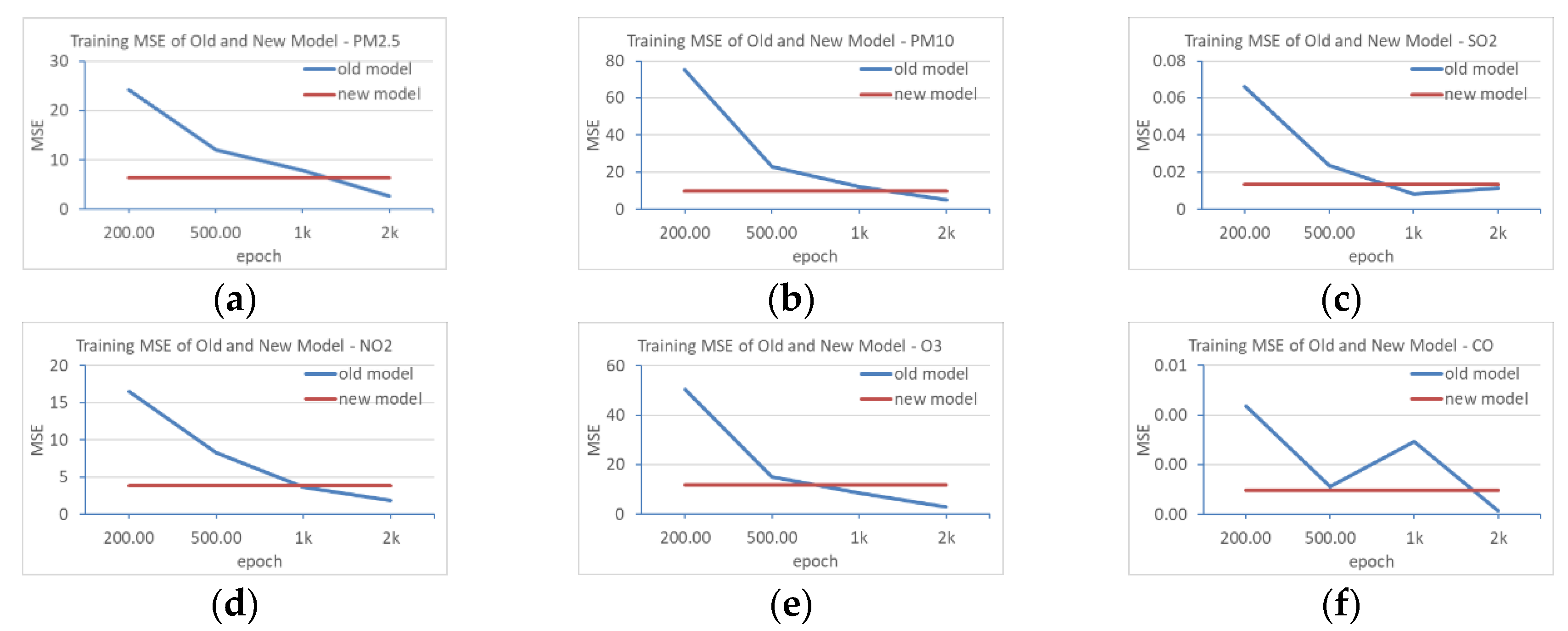
During the training of each set of models, the mean squared error MSE
(Training) is calculated. From evaluating these MSE
(Training)’s, it is possible to explore how well a model is trained and to what level the different hyperparameters improve the models with the same designed architecture. This research aims to understand how the newly proposed MTS-DR model can speed up and improve the training process and efficiency. As shown in
Figure 8, the MTS-DR model trains as well as the old model at epoch numbers of 1000 and 2000. It seems that the old model outperforms the MTS-DR model for 2000 epochs with these MSE
(Training)’s. However, these are the MSE
(Training)’s for training processes. In the following sections, it can be found that the MTS-DR model still performs better in predictions. It should be noted that, in
Figure 8, this MSE
(Training) is only for the training process and does not fully represent the prediction performance of the model because each model is trained quite accurately. This is just a reference indicator to help select hyperparameters so that the experiment can be stopped in a certain situation.
4. Discussion
As mentioned above, after inspecting each group of models, which are trained under the given test settings and conditions, the next step is to use the test set data to test their ability to predict future values.
Figure 7 shows the comparison of the actual data, the predicted data of the original old model, and the predicted data of the newly proposed MTS-DR model, where the blue curve is the actual data, the green curve is the predicted data of the original old models, and the orange curve is the predicted data of the proposed MTS-DR model (i.e., the MTS-DR model trained in three independent iterations for three sets of decomposed time series and used to predict the original MTS, namely the trend, seasonality, and residual components of the MTS). In addition, as mentioned earlier, because MSE
(Training) is 0, there is no need to train the seasonal components. Therefore, the seasonal components used here are the same set of time series data as the original decomposed seasonal component.
Compare the actual data, the predicted data by the original old model, and the predicted data by the proposed MTS-DR model. The blue curve is the actual data, while the green curve is the predicted data by the original old model, and the orange color curve is the predicted data by the proposed MTS-DR model, i.e., train and predict the MTS in three iterations for the trend, seasonal, and residual components of the MTS, respectively.
Table 2,
Table 3 and
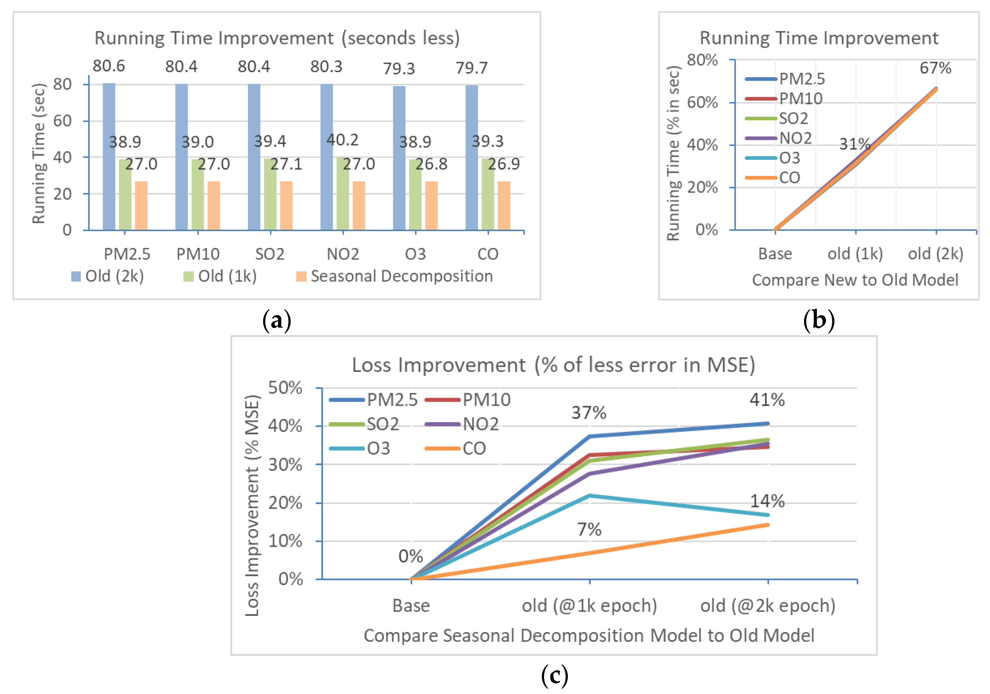
Table 4 are the final metrics of all experimental results for the concentration of those six air pollutants. After calculating and comparing all the prediction values, i.e., the part of the test set beyond the right side, in terms of the prediction of the concentration of six air pollutants, the newly proposed MTS-DR model approach has improved both in terms of prediction accuracy and training time; e.g., for PM2.5, the time needed to train the old model at 1000 epochs is 38.94 s, while that for the MTS-DR model is 27.01 s (i.e., the summation of the training time of the sub-models of trend, seasonal, and residual components). Forecasting results using decomposed time series models are significantly better, often due to the fact that the algorithm can analyze those decomposed data with better symmetry and compact support for multi-sub-layer data, which have little signal aliasing [
21].
The percentage increase in efficiency and performance in this area is significant. The accuracy has improved from 37% to 41%, 32% to 35%, 31% to 37%, 28% to 35%, 17% to 22%, and 7% to 14% for PM
2.5, PM
10, SO
2, NO
2, ozone, and CO, respectively. The training time is reduced from 31% to 66% for all six air pollutant elements (see
Figure 9). How to shorten the running time is helpful sometimes when the system is designed for real-time monitoring. The big O is a common method to measure and estimate the running time. For the training time of an ANN-type model, if the algorithm adopted is simple, the big O will be O(
n) so that if the multivariate input size increases, the running time will be multiple, e.g., the time needed will increase from
t to 10
t when the input size increases from 1 to 10. However, if the model is complicated and has an algorithm that leads to a large O
O(
n2), then the running time will be exponentially increased to 10
2 ×
t, i.e., from
t to 100
t. Thus, the reduction in the number of epochs could be a significant contribution to the performance of the ANN-type models.
As mentioned before, in
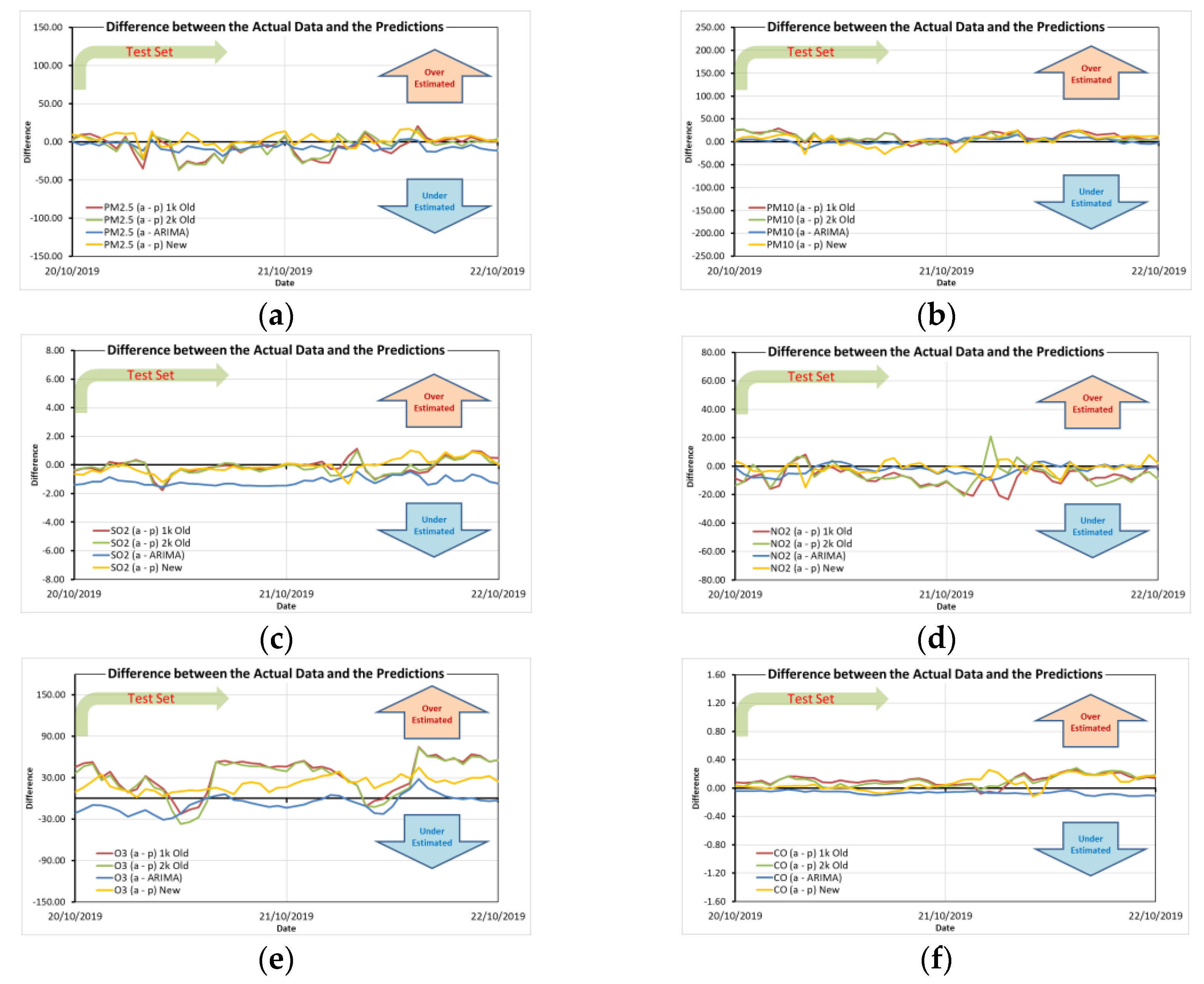
Figure 7, the model trained in the experiment is used to make predictions. The prediction ability of the new model is satisfactory. Even though ARIMA seems to be close to it in terms of error calculation, under visualization, it can be easily seen that its predictions are generally small, do not change much, and cannot reflect well. The realistic 24 h oscillation period changes. The new model also predicts trend changes in many places.
Figure 10 illustrates this point better, which shows the difference between the predicted values of each model and the actual observed values within 48 h. In terms of predicting air quality, if it can be predicted for 48 h, it is sufficient to assist decision-making. Just like its commonality, this time step is sufficient even if it is applied in other fields. Today’s real-time adaptive systems require that the model be continuously retrained and updated with hyperparameters.
Although the prediction range is temporarily based on 8:2 of the length of the total dataset to be the test set, the practical prediction time is generally the future 48 h. As this research result will be incorporated into an adaptive feature engineering module for a larger project, the model can be retrained with newly observed data to improve accuracy for operational tasks. Therefore, in
Figure 10, the error value of the proposed model is always closest to the zero value of the central axis. If it is upward, there is an overestimation of the actual situation, while downward is an underestimation. While the other models, i.e., the three curves of red, green, and blue, all deviate further upwards and downwards, the error value of the proposed model, i.e., the yellow curve, always hovers closest to the zero value of the central axis. Therefore, the proposed model always maintains the highest accuracy level. It can be seen that the newly proposed MTS-DR model can not only greatly reduce training time and enable instantaneous adaptive feature engineering, but also achieve a slight improvement in accuracy.
5. Conclusions
It is concluded that when forecasting time series data using deep learning models, since each type of MTS has very different characteristics, it is necessary to analyze the MTS in advance, which helps in model construction and efficiency. In this research, the case study focuses on air quality forecasting in small cities. Finally, all the final forecast results are visualized. Although the error level of ARIMA is very close to that of the MTS-DR model, the MTS-DR model is better at predicting key changes in air pollutant concentrations at many critical points. For many locations where the trend changes, the forecast is ideal, but accurate forecasting of peaks remains a challenge. Experiments show that the proposed MTS-DR model can significantly speed up the training time as well as slightly reduce error loss, that is, improve the accuracy rate. It is easier to train the trend component as it is simpler than the original, while there is no need to train the seasonal component as the MSE for this is always zero. The training of the residual is still the most difficult part, with more uncertainty. Nevertheless, the new proposed MTS-DR model can still benefit from the former two factors. Thus, the proposed MTS-DR is helpful for adaptive public alerting services with the advantage of the shortest training time, which is crucial for a real-time model that relies on adaptive feature engineering.
Techniques such as wavelet analysis, Fourier analysis, auto-correlation, etc. are very useful for identifying different degrees of oscillation and seasonality. In this case, auto-correlation is used to visualize and explore the MTS with its 24 h oscillations or seasonality. It can be seen that the weather elements and the concentration of atmospheric pollutants affected by the weather have a 24 h seasonality. There may be some periods when this seasonality is not apparent due to severe weather, unusual atmospheric phenomena, or human activities that affect the normal diffusion or dispersion of air pollutants.
Future work will include the binding and handling of those abnormal and special weather conditions, namely typhoons, rainy seasons, heavy rain, sandstorms, and monsoons. Now, when analyzing the acquired data source, if some extreme data are found at this initial stage, just consider it an outlier for the whole time series. Combining artificial intelligence-based models with numerical model simulations can improve forecasting capabilities for complex weather [
22]. Furthermore, this study is part of the adaptive feature engineering in our final project, which is an adaptive public service.
Author Contributions
Conceptualization, B.C.M.T., S.-K.T. and A.C.; methodology, B.C.M.T., S.-K.T. and A.C.; software, B.C.M.T., S.-K.T. and A.C.; validation, B.C.M.T., S.-K.T. and A.C.; formal analysis, B.C.M.T., S.-K.T. and A.C.; investigation, B.C.M.T., S.-K.T. and A.C.; resources, B.C.M.T.; data curation, B.C.M.T.; writing—original draft preparation, B.C.M.T.; writing—review and editing, B.C.M.T., S.-K.T. and A.C.; visualization, B.C.M.T.; supervision, S.-K.T. and A.C.; project administration, B.C.M.T., S.-K.T. and A.C. All authors have read and agreed to the published version of the manuscript.
Funding
This work is funded by the FCT—Foundation for Science and Technology, I.P./MCTES through national funds (PIDDAC), within the scope of CISUC R&D Unit—UIDB/00326/2020 or project code UIDP/00326/2020. This work is supported in part by the research grant (No.: RP/FCA-09/2023) offered by Macao Polytechnic University.
Institutional Review Board Statement
Not applicable.
Informed Consent Statement
Not applicable.
Data Availability Statement
The partial of datasets are online from third parties and partial analyzed during the current study are not publicly available due to the sensitive characteristics but are available from the corresponding author on reasonable request. The code is mainly composed in standard packages of Pytorch and MatLab, and available from the corresponding author on reasonable request.
Acknowledgments
This work is funded by the FCT—Foundation for Science and Technology, I.P./MCTES through national funds (PIDDAC), within the scope of CISUC R&D Unit—UIDB/00326/2020 or project code UIDP/00326/2020. This work is supported in part by the research grant (No.: RP/FCA-09/2023) offered by Macao Polytechnic University.
Conflicts of Interest
The authors declare no conflicts of interest.
References
- Tam, B.C.M.; Tang, S.K.; Cardoso, A. Evaluation of ANN Using Air Quality Tracking in Subtropical Medium-Sized Urban City. In Proceedings of the 2022 5th International Conference on Pattern Recognition and Artificial Intelligence (PRAI), Chengdu, China, 19–21 August 2022; pp. 153–158. [Google Scholar] [CrossRef]
- Chaudhary, V.; Deshbhratar, A.; Kumar, V.; Paul, D. Time Series Based LSTM Model to Predict Air Pollutant’s Concentration for Prominent Cities in India. In Proceedings of the UDM’18, London, UK, 20 August 2018. [Google Scholar]
- Vanos, J.K.; Cakmak, S.; Kalkstein, L.S.; Yagouti, A. Association of Weather and Air Pollution Interactions on Daily Mortality in 12 Canadian Cities. Air Qual. Atmos. Health 2015, 8, 307–320. [Google Scholar] [CrossRef] [PubMed]
- Cruz, A.M.J.; Alves, C.; Gouveia, S.; Scotto, M.G.; Freitas, M.d.C.; Wolterbeek, H.T. A Wavelet-Based Approach Applied to Suspended Particulate Matter Time Series in Portugal. Air Qual. Atmos. Health 2016, 9, 847–859. [Google Scholar] [CrossRef]
- Gaizen, S.; Fadi, O.; Abbou, A. Solar Power Time Series Prediction Using Wavelet Analysis. Int. J. Renew. Energy Res. 2020, 10, 1767–1773. [Google Scholar] [CrossRef]
- Fang, C.; Gao, Y.; Ruan, Y. Improving Forecasting Accuracy of Daily Energy Consumption of Office Building Using Time Series Analysis Based on Wavelet Transform Decomposition. IOP Conf. Ser. Earth Environ. Sci. 2019, 294, 012031. [Google Scholar] [CrossRef]
- Cao, D.; Wang, Y.; Duan, J.; Zhang, C.; Zhu, X.; Huang, C.; Tong, Y.; Xu, B.; Bai, J.; Tong, J.; et al. Spectral Temporal Graph Neural Network for Multivariate Time-Series Forecasting. Adv. Neural Inf. Process. Syst. 2020, 33, 17766–17778. [Google Scholar]
- Feng, X.; Li, Q.; Zhu, Y.; Hou, J.; Jin, L.; Wang, J. Artificial Neural Networks Forecasting of PM2.5 Pollution Using Air Mass Trajectory Based Geographic Model and Wavelet Transformation. Atmos. Environ. 2015, 107, 118–128. [Google Scholar] [CrossRef]
- Tsakiri, K.G.; Zurbenko, I.G. Prediction of Ozone Concentrations Using Atmospheric Variables. Air Qual. Atmos. Health 2011, 4, 111–120. [Google Scholar] [CrossRef]
- Yi, K.; Zhang, Q.; Cao, L.; Wang, S.; Long, G.; Hu, L.; He, H.; Niu, Z.; Fan, W.; Xiong, H. A Survey on Deep Learning Based Time Series Analysis with Frequency Transformation. arXiv 2023, arXiv:2302.02173. [Google Scholar]
- Rahimpour, A.; Amanollahi, J.; Tzanis, C.G. Air Quality Data Series Estimation Based on Machine Learning Approaches for Urban Environments. Air Qual. Atmos. Health 2021, 14, 191–201. [Google Scholar] [CrossRef]
- Hu, J.; Chen, Y.; Wang, W.; Zhang, S.; Cui, C.; Ding, W.; Fang, Y. An Optimized Hybrid Deep Learning Model for PM2.5 and O3 Concentration Prediction. Air Qual. Atmos. Health 2023, 16, 857–871. [Google Scholar] [CrossRef]
- Zhang, J.; Li, S. Air Quality Index Forecast in Beijing Based on CNN-LSTM Multi-Model. Chemosphere 2022, 308, 136180. [Google Scholar] [CrossRef] [PubMed]
- Das, B.; Dursun, Ö.O.; Toraman, S. Prediction of Air Pollutants for Air Quality Using Deep Learning Methods in a Metropolitan City. Urban Clim. 2022, 46, 101291. [Google Scholar] [CrossRef]
- ECMWF (European Centre for Medium-Range Weather Forecasts) Climate Data Store. Available online: https://cds.climate.copernicus.eu (accessed on 20 March 2024).
- SMG (Direcção dos Serviços Meteorológicos e Geofísicos de Macau) Concentration of Pollutants. Available online: https://www.smg.gov.mo/en/subpage/181/airconcentration (accessed on 20 March 2024).
- SMG (Direcção dos Serviços Meteorológicos e Geofísicos de Macau) Present Weather. Available online: https://www.smg.gov.mo/en/subpage/73/actualWeather (accessed on 20 March 2024).
- Rezaei, H.; Faaljou, H.; Mansourfar, G. Stock Price Prediction Using Deep Learning and Frequency Decomposition. Expert Syst. Appl. 2021, 169, 114332. [Google Scholar] [CrossRef]
- Feng, Z.K.; Niu, W.J.; Tang, Z.Y.; Jiang, Z.Q.; Xu, Y.; Liu, Y.; Zhang, H. Monthly Runoff Time Series Prediction by Variational Mode Decomposition and Support Vector Machine Based on Quantum-Behaved Particle Swarm Optimization. J. Hydrol. 2020, 583, 124627. [Google Scholar] [CrossRef]
- Seabold, S.; Perktold, J. Statsmodels: Econometric and Statistical Modeling with Python. In Proceedings of the 9th Python in Science Conference (SciPy 2010), Austin, TX, USA, 28–30 June 2010; pp. 92–96. [Google Scholar] [CrossRef]
- Liu, H.; Long, Z. An Improved Deep Learning Model for Predicting Stock Market Price Time Series. Digit. Signal Process. A Rev. J. 2020, 102, 102741. [Google Scholar] [CrossRef]
- Ian, V.K.; Tse, R.; Tang, S.K.; Pau, G. Transforming from Mathematical Model to ML Model for Meteorology in Macao’s Smart City Planning. In Proceedings of the 2023 7th International Conference on E-Commerce, E-Business and E-Government, Online, 27–29 April 2023; pp. 72–78. [Google Scholar]
| Disclaimer/Publisher’s Note: The statements, opinions and data contained in all publications are solely those of the individual author(s) and contributor(s) and not of MDPI and/or the editor(s). MDPI and/or the editor(s) disclaim responsibility for any injury to people or property resulting from any ideas, methods, instructions or products referred to in the content. |
© 2024 by the authors. Licensee MDPI, Basel, Switzerland. This article is an open access article distributed under the terms and conditions of the Creative Commons Attribution (CC BY) license (https://creativecommons.org/licenses/by/4.0/).


