
A Static Security Region Analysis of New Power Systems Based on Improved Stochastic–Batch Gradient Pile Descent

State Centre for Engineering Research, Ministry of Education for Renewable Energy Generation and Grid-Connected Control (Xinjiang University), Urumqi 830047, China
*
Author to whom correspondence should be addressed.
Appl. Sci. 2024, 14(9), 3730; https://doi.org/10.3390/app14093730
Submission received: 5 March 2024
/
Revised: 18 April 2024
/
Accepted: 24 April 2024
/
Published: 27 April 2024
(This article belongs to the Section Electrical, Electronics and Communications Engineering)
Abstract
:The uncertainty in the new power system has increased, leading to limitations in traditional stability analysis methods. Therefore, considering the perspective of the three-dimensional static security region (SSR), we propose a novel approach for system static stability analysis. To address the slow training speed of traditional deep learning algorithms using batch gradient descent (BGD), we introduce an improved stochastic–batch gradient descent (S-BGD) search method that combines the advantages of stochastic gradient descent (SGD) in fast training. This method ensures both speed and precision in parameter training. Moreover, to tackle the problem of getting trapped in local optima and saddle points during parameter training, we draw inspiration from kinematic theory and propose a gradient pile (GP) training method. By utilizing accumulated gradients as parameter corrections, this method effectively avoids getting stuck in local optima and saddle points, thereby enhancing precision. Finally, we apply the proposed methods to construct the static security region for the IEEE-118 new power system using its data as samples, demonstrating the effectiveness of our approach.
1. Introduction
With the large-scale integration of renewable energy sources, the intermittent and fluctuating nature of their output has made power grid operation more complex and variable. As a result, the construction of the static security region (SSR) has become increasingly challenging [1]. Ensuring the static stability of power systems has become an urgent problem to be addressed. Traditional point-by-point methods are no longer sufficient to meet the construction demands of the SSR under the high penetration rate of renewable energy [2,3]. Therefore, research on stability analysis methods suitable for the current complex power systems holds significant practical importance [4]. In order to more accurately and efficiently analyze the static stability of the system, Jarjis and others proposed the method of power system static security region analysis in 1975 [5].
The static security region (SSR) in power systems is a collection of all possible operational points that maintain stability under given operating conditions. Each point within this region represents a state of the power system where it can operate safely without violating any electrical parameters, such as voltage, power, frequency, etc. States within the SSR mean that the grid can stably meet load demands without being affected by external disturbances. The concept of the static security domain is crucial for the planning, operation, and control of power systems, especially in scenarios where a high proportion of new energy sources, such as wind and solar power, are integrated into the grid, making the determination of the SSR more important and complex. It provides grid operators with a visualization tool to monitor and assess the stability boundaries of the system, and finding stable operating critical points quickly is the primary challenge in constructing the static security region [6]. In the literature [7], the method based on the Lagrange multiplier is proposed to trace the Security Region Boundary (SRB) to construct the SSR. In the literature [8], the efficiency of constructing the SSR is improved by optimizing the search model based on the properties of the power grid boundary. The literature [9] approximates the SSR through the relationship between the spatial angles of the critical point’s space static security domain mathematical model tangent vector and the maximum spatial angle threshold. The literature [10] solves the security region using the Taylor series trajectory sensitivity method. The literature [11] uses based least absolute shrinkage and selection operator (Lasso) for optimal power flow calculation. All of the above studies aim to improve the efficiency and accuracy of constructing the security domain, but they do not consider the construction of the security domain under the scenario of new energy integration into the system.
In addition, intelligent optimization algorithms are commonly utilized in power system analysis. The gradient descent algorithm is a type of iterative optimization algorithm that can be applied to solve linear or nonlinear problems. Depending on the different data usage approaches, such as data size, time complexity, and algorithm accuracy, the gradient descent algorithm can be categorized into the following distinct forms: (1) the batch gradient descent (BGD) algorithm; (2) the stochastic gradient descent (SGD) algorithm; and (3) the Mini-Batch Gradient Descent (MBGD) algorithm.
The literature [12] proposes the BGD algorithm, which computes the gradient of the cost function using the entire dataset during each iteration. However, with the growth of massive datasets and memory limitations, loading all the data at once becomes increasingly impractical, leading to slow training processes. Addressing the low efficiency of gradient descent in handling large-scale samples, the literature [13] introduces the SGD algorithm, which calculates the gradient using only a single sample during each iteration to update the parameters, eliminating computational redundancy. However, the process introduces more noise, causing not every iteration to converge towards the global optimum and reducing training accuracy.
To overcome the shortcomings of the two methods mentioned above, the literature [14] presents the Mini-Batch Gradient Descent algorithm, which uses a fixed number of training samples to form a small sample set during each parameter update. The learning rate of the parameter is affected not only by the learning rate parameter η but also by the value of the mini-batch size m. However, when the value of m is too large, the parameter update becomes slower, and achieving the same accuracy requires a significantly increased cost.
To further accelerate the parameter update rate of the gradient descent algorithm and escape from the attraction basin of local minima, the literature [15] proposes the Momentum Learning Rate as a supplementary term in the parameter update formula of the gradient descent algorithm. It accumulates the historical gradients throughout the parameter update process to influence the current direction of gradient descent.
Furthermore, the literature [16] introduces a pipelined stochastic gradient descent with Taylor expansion. The proposed method generates multiple model replicas to solve the weight inconsistency problem and adopts a Taylor expansion-based gradient prediction algorithm to mitigate the delayed gradient problem. The literature [17] designs a projection sub-gradient method based on the Nesterov accelerated gradient algorithm, which can achieve stable learning accuracy while maintaining convergence speed. The literature [18] builds on the idea of variance reduction and designs the distributed implementation algorithm Dis-SAGD, which employs an adaptive sampling strategy and momentum acceleration to achieve near-linear acceleration in distributed clusters. Lastly, the literature [19] utilizes mini-batch samples instead of all samples during the training process and performs batch subtraction updates while computing average gradients, resulting in the variance-reduced BSUG algorithm.
The batch gradient descent method targets the entire dataset and has the ability to search for global optimal solutions, but it comes with a high computational cost and slow training speed. On the other hand, the Mini-Batch Gradient Descent method divides the large dataset into several small subsets and computes the gradient only for a specific small subset during each iteration. This effectively reduces the computational workload per iteration and improves computational efficiency. The stochastic gradient descent method treats each sample as a small subset, and both Mini-Batch Gradient Descent and stochastic gradient descent methods can be considered as types of it. While the stochastic gradient descent method efficiently searches for the optimal parameter region, it may fall short in finding the global optimal solution.
Current research has delved deeply into improving the efficiency and accuracy of constructing safety domains, but there has been less consideration of the impact of large-scale new energy integration and penetration rates on the boundaries of power system safety domains. Addressing the shortcomings of fitting accuracy in stochastic gradient descent and the insufficient training efficiency of batch gradient descent, this study utilizes the fast training speed of stochastic gradient descent and the high fitting accuracy of batch gradient descent to improve traditional gradient descent algorithms. We propose an improved stochastic–batch gradient descent method and a gradient accumulation strategy, applying them to the construction of the static safety domain in power systems incorporating new energy. The method is used to track critical stable operating points within the safety domain, forming the SSR and conducting static stability analysis of the system. Through this method, this paper aims to achieve the following contributions. First, it aims to enhance the accuracy and efficiency of static safety domain analysis in new energy power systems. Second, it aims to explore the characteristics of changes in the static safety domain boundaries of power systems under different wind power penetration rates. Finally, through case study analysis, it aims to validate the practical utility of the proposed methods and provide new insights for power system stability research.
2. Research on the Static Security Region (SSR) of Power Systems Based on New Energy
The static security region of a power system is defined as the collection of all stable operating points. It approaches the problem from a domain perspective, describing the region where the system can operate safely and stably as a whole. The relative relationship between system operating points and the boundaries of the security region provides information on safety margins and optimal control, enabling more efficient analysis of the static stability of the power system. It is typically represented by a set of operating points that satisfy the power flow equations and various security constraints of the power system. Mathematically, the SSR can be represented as follows [20]:
In the provided description, represents the vector of system state variables. represents the vector of injected power at each node. denotes the system power flow equations. and are the sets of system nodes and generator nodes, respectively. and are the minimum and maximum allowable voltage magnitudes at each node. and are the minimum and maximum active power output limits of the generators. and are the minimum and maximum reactive power output limits of the generators. and represent the active power limits in the forward and reverse directions, respectively, of transmission lines i − j.
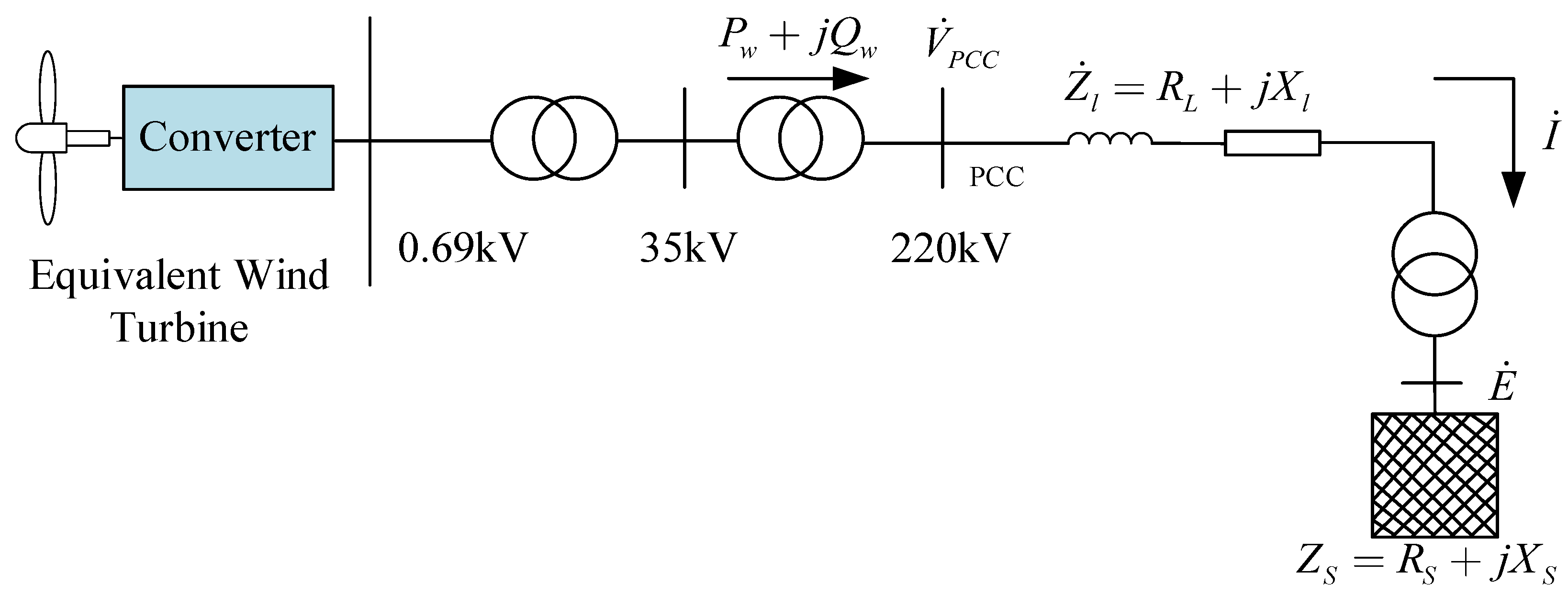
Considering the integration of new energy sources and deriving an analytical expression for the system’s static security region based on static power flow calculations, the equivalent schematic diagram of wind farm integration into the grid is illustrated in Figure 1.
In the diagram, represents the voltage at the wind power access point in the system, represents the voltage at the wind farm grid connection point, represents the equivalent impedance of the system, represents the equivalent impedance of the transmission line between the wind farm grid connection point and the system equilibrium point, represents the apparent power of the wind farm, and represents the injected current from the wind farm. The relationship between wind farm active power output and voltage curve is derived as follows:
For the given load on the busbar, , .
The apparent power of the wind farm is given by
In Equation (3)
Simplifying Equation (3), we obtain
Organizing Equation (6), we obtain
Solving for , , and in Equation (7), we obtain the expression for the static security domain as follows:
The assignment of values in Equation (8) should satisfy the following two constraint conditions.
(1) Equality constraint condition
The expression represents the equality constraint, ensuring power balance between supply and demand, where denotes the total number of system nodes and G denotes the number of generator nodes, and it can be represented as follows:
In Expression (9), x represents the system’s state variables, y denotes the injected power at nodes, and and represent the active and reactive power injection at node i, respectively. and are the real and imaginary parts of the admittance of branch , and is the phase angle difference between the two terminal nodes of branch .
(2) Inequality constraints
When the system experiences voltage fluctuations caused by disturbances, the voltage at the grid connection point is maintained by dynamically adjusting the reactive power sources within the wind farm. The introduced constraint for the voltage deviation at the wind farm connection point is as follows:
where VPCC represents the actual voltage at the wind farm connection point; denotes the commanded voltage at the connection point; and signifies the permissible control error.
The reactive regulation capacity constraint of wind turbines is as follows:
The symbol represents the dead band for PCC bus voltage control.
The inequality constraints for the wind farm also include voltage magnitude constraints for each node.
The symbols and represent the minimum and maximum values of the node voltage magnitude, respectively.
The active power constraint for the branch is given by
and are the positive and negative active output limits of branch , respectively.
The reactive power constraint for branches is as follows:
Let , where is the (i,j)-th element of the nodal admittance matrix. Therefore
Assuming ; is small; therefore, and . Equation (14) can be written as follows:
Taking the modulus of both sides in Equation (15), we obtain
The constraint expressed by the voltage phase difference at both ends of branch can be obtained from the current constraint, namely
In conclusion, the reactive power flow constraint is as follows:
The static security domain obtained in Equation (8) and its constrained conditions, (9) to (19), requires an optimization algorithm for global parameter identification. In this paper, we employ the gradient descent algorithm, which offers fast computational speed and excellent global optimization capability for addressing large-scale mathematical optimization search problems, as detailed in Section 2 and Section 3.
The equation for the safety domain hyperplane can be expressed in the following form:
In Equation (20), represents the coefficients of the hyperplane to be determined, y denotes the dimension of the system, and y is the observed variable (usually 1).
For the m critical points found during the search , and their errors can be represented as follows:
In Equation (21)
The error vector should satisfy Equation (23)
Taking the partial derivative with respect to to , we have
The least squares estimate for parameter can be solved as follows:
In order to evaluate the accuracy of the approximation, it is necessary to calculate the fitting error for each critical point on the hyperplane. The fitting error , as shown in the equation above, can be calculated using the following formula:
The distance from the critical point to the boundary (taken as an absolute value) is
represents the module of the critical point .
As long as m ≥ n, the least squares solution will have a unique solution. To ensure fitting accuracy, it is necessary to search for m ≥ 2n critical points.
3. Improved Stochastic–Batch Gradient Pile Descent
The GD algorithm can be divided into three different forms: BGD, MBGD, and SGD. In order to overcome the slow training speed of BGD and fully utilize the advantages of the fast search for the optimal parameter region using SGD, this paper proposes an improved stochastic–batch gradient descent method (S-BGD). Additionally, to address the issue of the traditional GD algorithm easily getting stuck in local optima and saddle points during training, a gradient accumulation strategy (GP) is introduced. Below, we will introduce these improvement methods separately.
3.1. The Improved Method Based on Stochastic–Batch Gradient Descent (S-BGD)
The fundamental idea of the S-BGD method is to utilize the efficiency of stochastic gradient descent (SGD) in the early stages of iteration to quickly search for the region where the global optimum lies. Once the search point reaches the vicinity of the global optimum region, the method switches to batch gradient descent (BGD) with a larger step size to efficiently search for the global optimum within the parameter space, thereby improving fitting accuracy. Figure 2 illustrates the optimization process of the S-BGD method for a model with two-dimensional variables as an example.
In Figure 2, the function L (x1, x2) represents the optimization objective of the model, where x1 and x2 are the optimization variables. The initial point is located at point A, and the global optimum is at point C. The parameter training starts using the SGD method in the early stages of optimization to quickly search for the optimal parameter region at point B. Subsequently, the BGD method is employed within the optimal parameter region with larger steps to search for the global optimum at point C. As shown, the S-BGD method combines the advantages of the fast parameter search capability of SGD and the ability of BGD to find the global optimum, thereby improving the training speed while ensuring fitting accuracy.
3.2. The Improvement Method Based on the Gradient Pile (GP)
In the traditional gradient descent (GD) algorithm, the optimization variable is updated using the negative gradient as the correction term in each iteration. For an unconstrained optimization model, the k-th iteration of the traditional GD algorithm is performed using the following formula:
In Equations (28) and (29), H is the objective function of the optimization model. is the optimization variable. represents the value of x at the k-th iteration. is the negative gradient of H with respect to . is the step size used in the iteration.
The traditional GD algorithm guides the optimization variable to find points where the gradient is zero and uses a gradient equal to zero as the convergence criterion. However, during parameter training, there are many local optimal points and saddle points in the solution space where the gradient is zero. If the gradient equal to zero is the only convergence criterion, the GD algorithm may get stuck in local optimal points and saddle point regions during the training process, reducing training accuracy. To address this problem, this paper proposes an improvement based on the accumulation of gradients as the correction term. The k-th iteration step is given by
In Equations (30)–(32), a and v, respectively, represent the negative gradient of x and its accumulation. and are weight parameters, and is the iteration step size. To ensure the convergence of the iterative computation, the accumulation of gradients should exhibit a decaying trend during the iteration process. Therefore, it is specified that .
It can be observed that using the gradient accumulation as the correction term and considering the gradient accumulation as 0 as the convergence criterion not only maintains the descent rate of the negative gradient but also effectively avoids getting trapped in saddle points and local optima. By doing so, it enables the search for the global optimal solution and thus enhances the optimization capability of the GD algorithm.
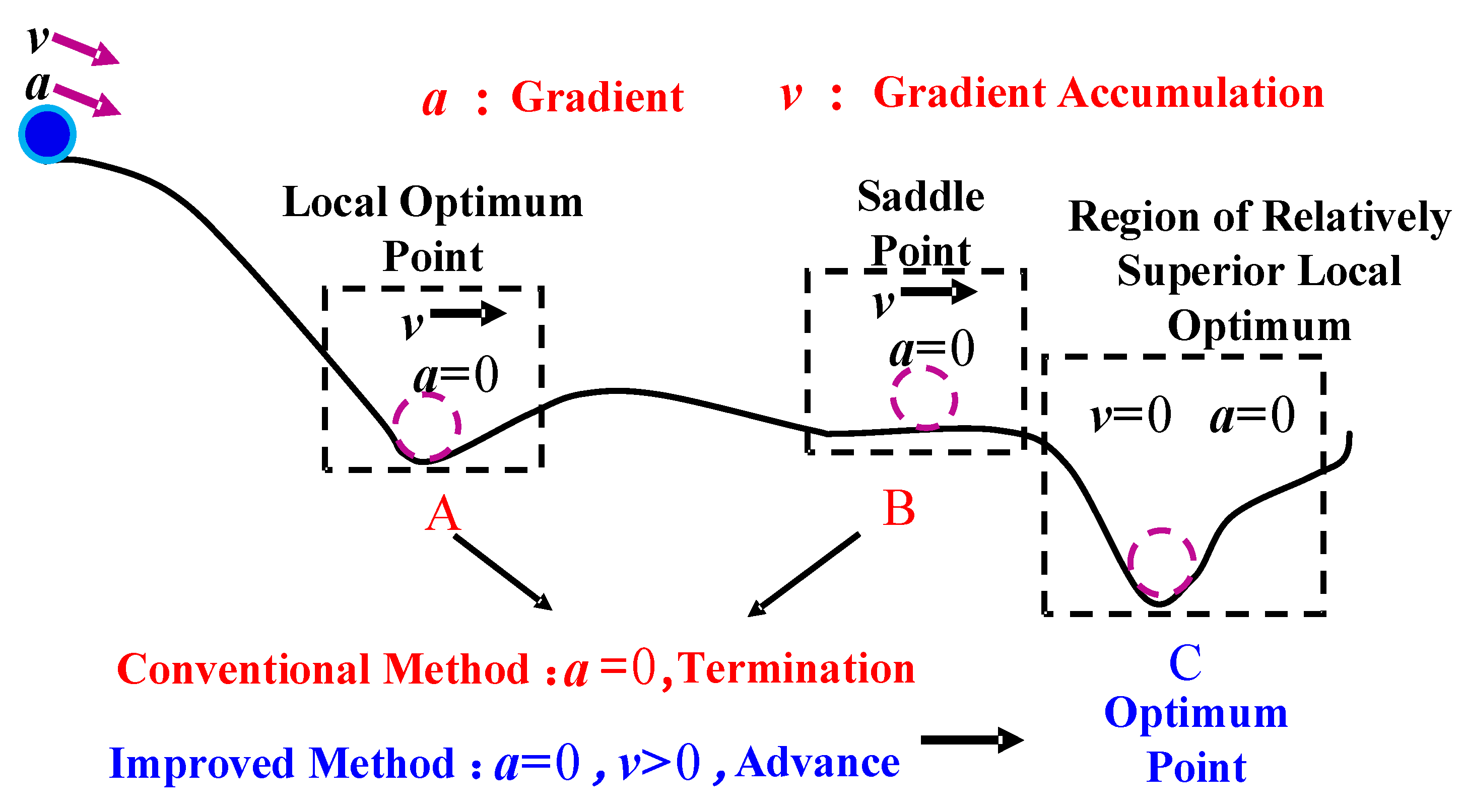
The search process based on gradient accumulation is illustrated in Figure 3. In the figure, a ball starts rolling down from the top of the hill, where the gradient accumulation is represented as and the negative gradient as . The negative gradient acts as an acceleration, guiding the motion of the ball. At the extremum point A and the saddle point B, the values of become 0. According to the traditional GD algorithm, the computation would end at either point A or B. However, as seen in Figure 3, the optimal point is actually C, not A or B. Thus, the traditional GD algorithm gets trapped in a local optimum or a saddle point. On the other hand, using the gradient accumulation-based search method proposed in this paper, when the ball reaches point A or B, it continues to move forward to point C, effectively avoiding the problem of getting stuck in local points or saddle points during the search process.
In conclusion, this paper proposes a comprehensive improvement in parameter training strategy by employing both the S-BGD and GP methods. This approach enhances training efficiency while effectively avoiding convergence to local points and saddle points. We refer to this enhanced method as the stochastic–batch gradient pile descent (S-BGPD) method. The S-BGPD method combines the SGD and GP methods in the early stages of training to quickly reach the optimal parameter region and then switches to BGD with GP to search for the global optimum.
4. A Methodology for Fitting Safety Domain Boundaries Based on the Improved Stochastic–Batch Gradient Pile Descent
4.1. The Establishment of a Hyperplane Equation
The methods for solving hyperplane equations include fitting methods, dimensionality reduction methods, restoration methods, and intercept methods, among others. In this paper, a combination of stochastic gradient descent and batch gradient descent is used to determine the coefficients of the hyperplane and construct the safety domain for the power system. The practical safety domain is composed of critical hyperplanes. A specific description of the hyperplane equation ground is given in Section 2, Equations (20)–(27).
4.2. Training Is Conducted Using the Stochastic–Batch Gradient Descent Method
The parameter training of models based on deep learning mainly consists of two steps. (1) Pre-training the parameters of each hidden layer in a feedforward manner to obtain initial values for each hidden layer’s parameters. (2) On the basis of pre-training, applying an algorithm to uniformly train all parameters to adjust the hidden layer parameters and ultimately obtain the output layer parameters.
In the context of deep learning algorithm structure, this study adopts a six-layer hidden layer configuration, with each hidden layer having 100, 80, 60, 40, 30, and 20 neurons respectively. The activation function used for the hidden layers is the sigmoid function, while the output layer utilizes a linear function as its activation function. The sigmoid function is a typical activation function used in neural networks and has proven to be effective. Its mathematical expression is given by Equation (33) as follows:
The model structure is illustrated in Figure 4.
In Figure 4, represents the input variables and output variables, where represents the influencing parameters such as power flow data, and y represents the critical point active power. , respectively, denote the number of neurons, activation function, weight, and bias of the i-th layer. represents the output of the i-th layer, which also serves as the input for the I + 1-th layer. represents the input to the model, and the output of the model is the output of the last layer .
There are two methods for layer-wise pre-training: unsupervised learning and supervised learning. Research has shown that the supervised learning approach for layer-wise pre-training yields better fitting results. Therefore, in this paper, we adopt the supervised learning method for layer-wise pre-training. Below, we illustrate the first step of pre-training, focusing on the parameters () of the first hidden layer in the predictive model, as shown in Figure 4. The training structure for the first and second layers is depicted in Figure 5.
First, construct a three-layer neural network, as shown in Figure 5a, where represent the weight matrix parameters and biases of the output layer. The training optimization model is given by Equations (34)–(36) as follows:
In Equations (34)–(36), and , respectively, represent the input variable and output variable of the j-th sample. is the total number of training samples, and represents the training error or loss function.
By employing the stochastic–batch gradient descent method for training, we can obtain the parameters that satisfy our objectives. Then, based on Equations (34)–(36), we can compute the output for the first hidden layer. The specific implementation steps are as follows.
(1) Firstly, randomly initialize the initial values of the parameter variables . Then, perform iterative calculations using a combination of the SGD and GP methods. In the k-th iteration of the j-th sample, the update for is as follows:
where ,, and represent the values of and its negative gradient and gradient accumulation at the k-th iteration. The iterative update calculations for can be found in Appendix B. The methods for computing gradients of parameter variables can be referred to in references [21,22,23,24,25,26].
(2) Subsequently, the values obtained from step (1) for are used as initial values, and the iterative calculation is performed using the BGD method and GP method combined. At the t-th iteration, the iterative update for is as follows:
The iterative update calculations for can be found in Appendix B.
After the iterative calculations are completed, we obtain the pre-training values for , as well as the output values of the samples at the first hidden layer. With the pre-training of completed, we construct a three-layer neural network, as shown in Figure 5b. We use as the input for the second hidden layer and apply the same training approach as in the first layer to train the parameters of the second hidden layer’s neurons. We repeat this process iteratively until the pre-training of all six hidden layers’ neuron parameters is completed.
After completing the pre-training of hidden layers 1 to 6, we proceed with the second step of training, which involves using the algorithm to perform unified training on all parameters. Through this process, we obtain the weight matrix parameters and bias for all the neurons in the model.
4.3. Solve the Boundary of the Safety Domain by Utilizing the Stochastic–Batch Gradient Pile Descent (S-BGPD) Method
Step One: Initialization in the simulation system involves selecting three stable operating points of the system as starting points for the search process. Taking the two-dimensional search as an example, we determine the search range and generate search directions. We perform searches in three directions, 15°, 45°, and 75°, from the baseline operating point. We also conduct searches along the ray direction from the spatial origin to the baseline operating point. These searches enable us to obtain the initial critical points.
Step Two: We use the stochastic gradient descent (SGD) method to iteratively calculate the parameter variables and apply gradient accumulation to adjust the calculation results. This process helps us find the region where the global optimum is located.
Step Three: Within this region, we employ the batch gradient descent (BGD) method to perform iterative calculations and apply gradient accumulation to adjust the calculation results. We obtain the hyperplane coefficients and credible hyperplane.
Step Four: Following the corresponding search methods in Step Two and Step Three, sequentially search for critical points until the number of critical points exceeds ‘n’. At this point, we can employ the least squares method for fitting operations.
Step Five: Validate whether the error of the obtained hyperplane meets the required criteria. If the criteria are met, proceed to Step Six. If not, return to Step Two for recalibration.
Step Six: Finally, with the hyperplane that meets the error criteria, construct the safety domain of the system.
At the initial operating points S1, S2, and S3, the first critical point is searched in the directions of 15°, 45°, and 75°, respectively. However, searching for the first critical point near its vicinity may lead to data getting trapped in a local minimum, requiring GP correction to improve the reliability of the results.
The flow chart of constructing security domains based on improved stochastic-batch gradient pile descent is shown in Figure 6.
5. Discussion
5.1. S-BGPD Is Used to Construct the SSR (Static Security Region)
In this example, the IEEE-118 system is used to construct the boundary of the hyperplane. Firstly, time domain simulation results are obtained using MATLAB software (9.10.0.1602886 R2021a) to gather the power flow data. Then, based on the constraints of the stochastic–batch gradient descent method for the hyperplane, the safety domain’s hyperplane is constructed. Finally, the optimal coefficients for the hyperplane are obtained.
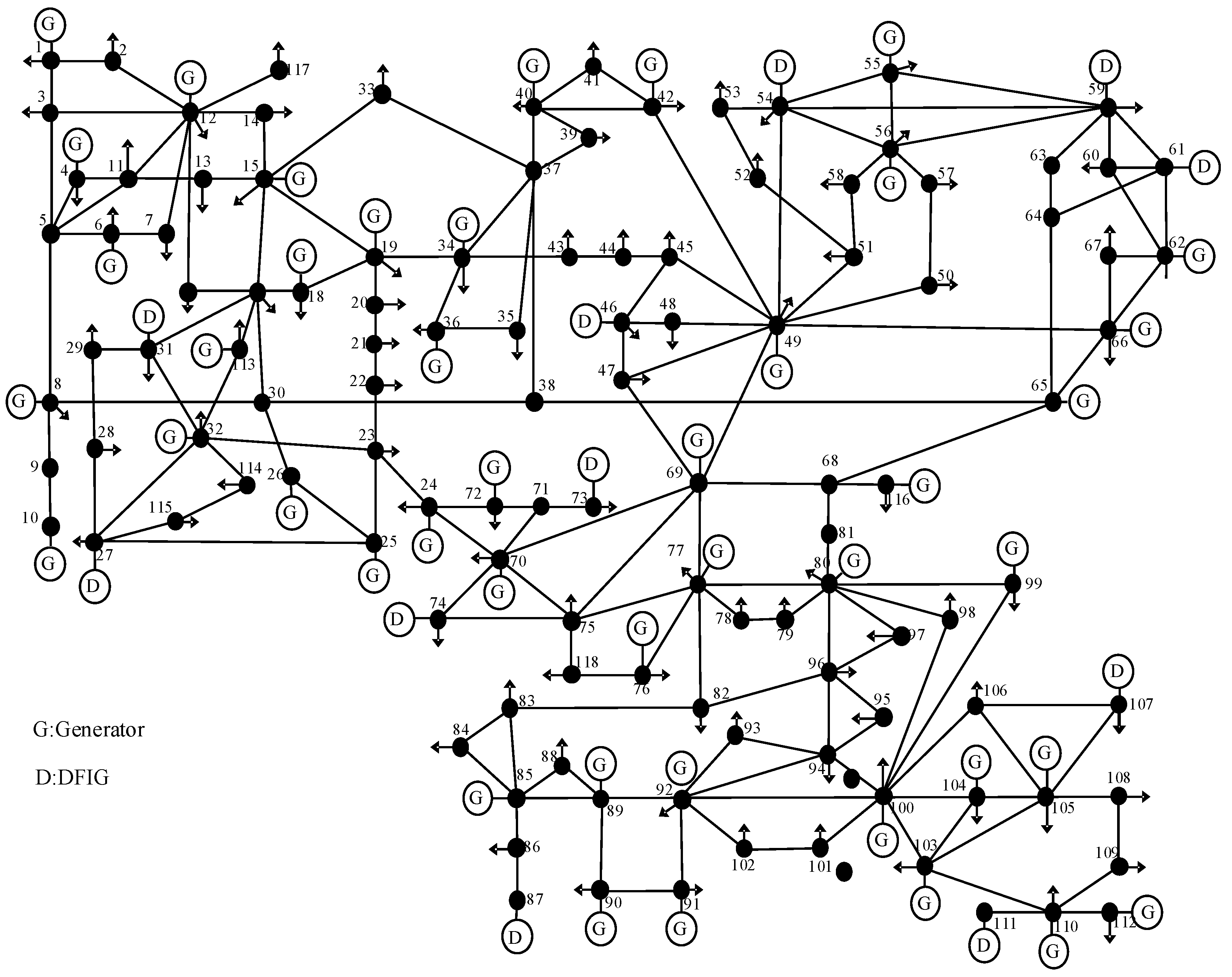
In the example of the IEEE-118 node system, the structure is illustrated in Figure 7.The system operates at a frequency of 50 Hz. The improved IEEE-118 node system consists of 186 transmission lines, 91 loads, and 54 generator units. The peak load of the system is 3733 MW. In this study, the penetration rate is set to 10 gradients with an increase of 5%, starting from an initial penetration rate of 5%.
The formula for calculating the new energy penetration rate, denoted as , is given as the ratio of the total new energy generation capacity to the overall power demand of the system, PL. The formula can be expressed as follows:
In the case study, ten nodes, namely, Node 27, Node 31, Node 46, Node 54, Node 59, Node 61, Node 73, Node 87, Node 111, and Node 107, are connected to wind power generation. These nodes are equipped with DFIG (Doubly Fed Induction Generator) wind turbines. Additionally, three critical nodes, G66, G103, and D27, are considered for the construction of the safety domain. Their active power output is used to create a three-dimensional vector to represent the safety domain.
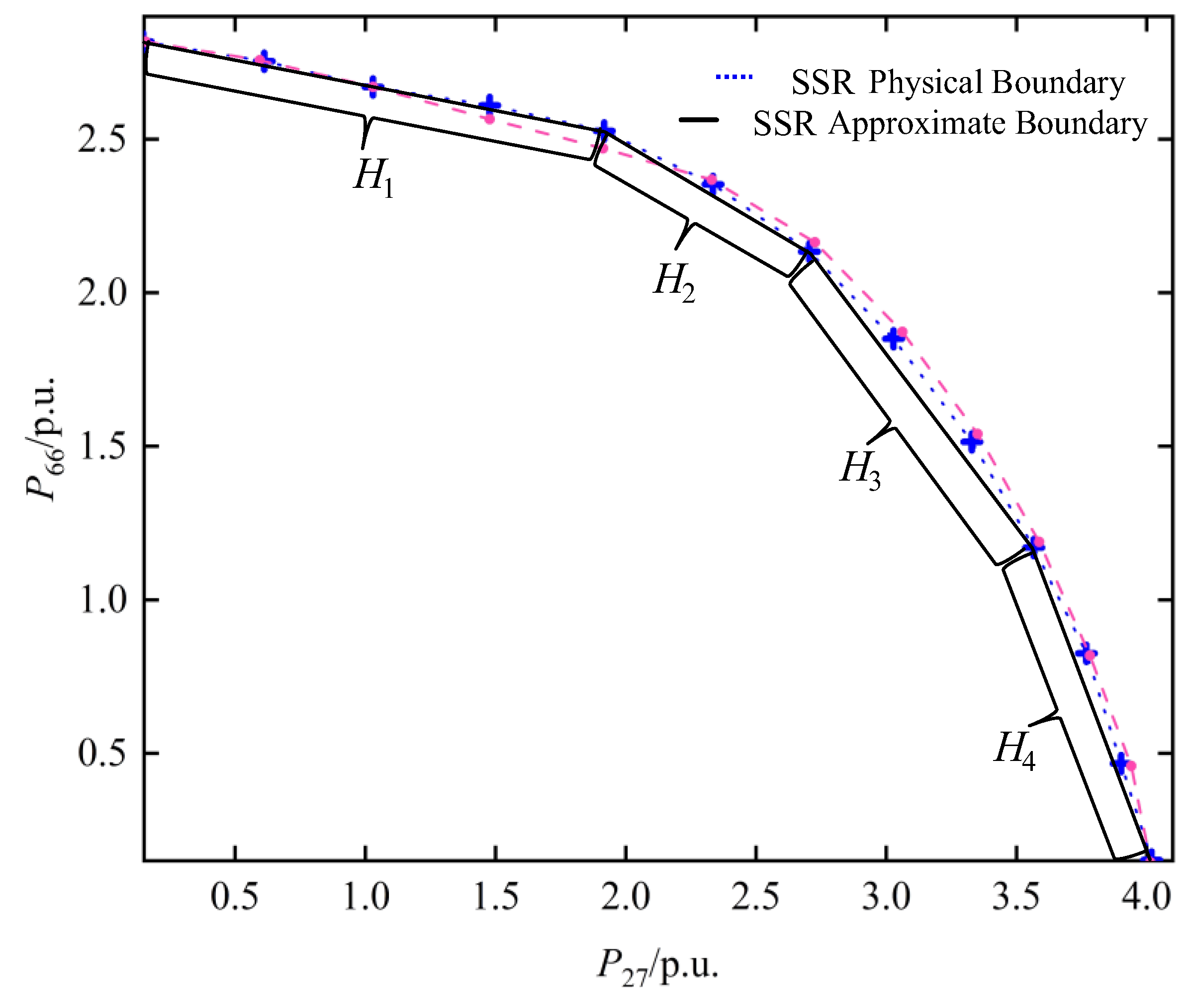
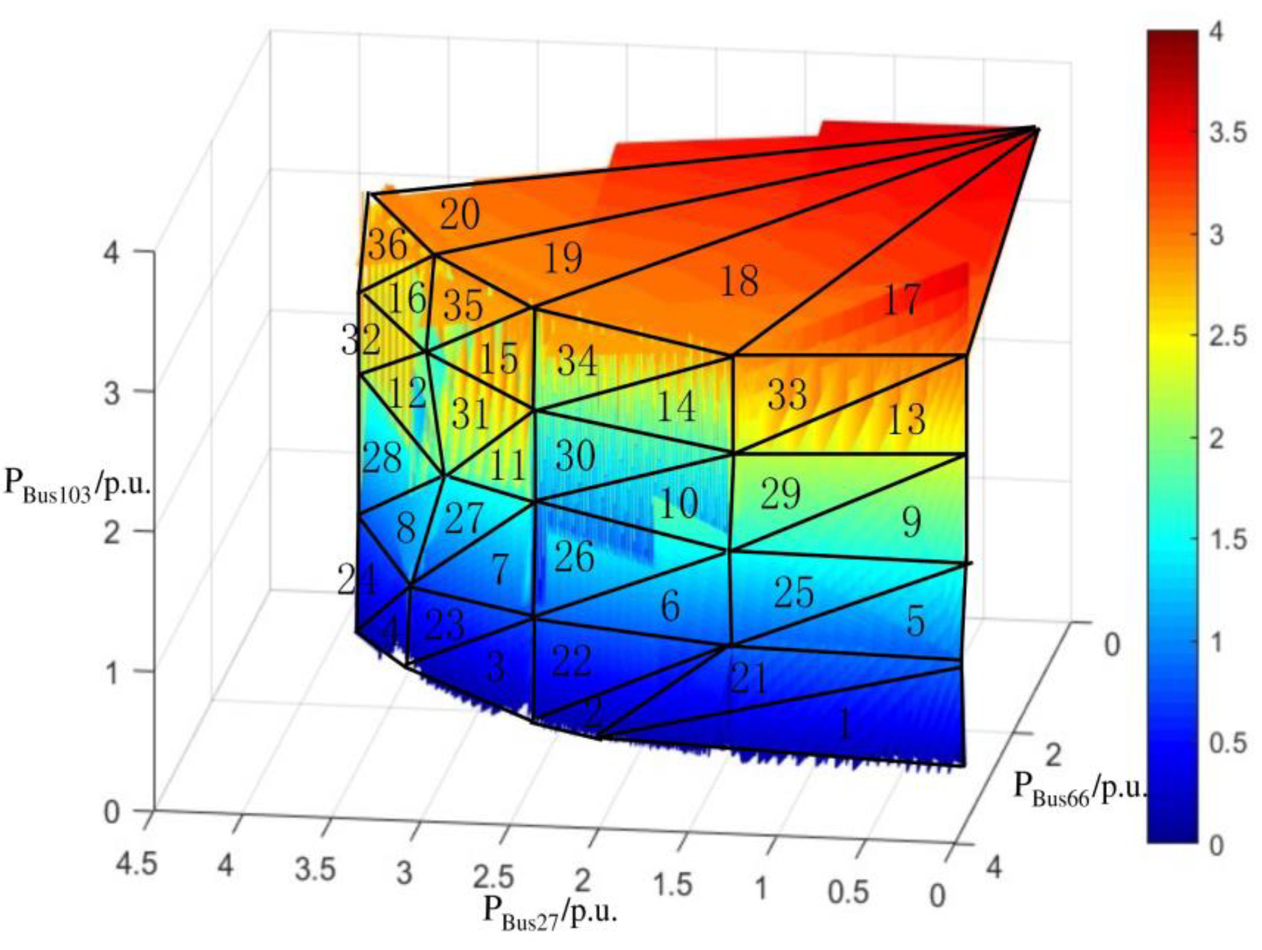
As an example, the boundary surface of the security domain fitted for a new energy penetration rate of 40% is shown in Figure 8 and Figure 9.
The nodes Bus 66 and Bus 27 are chosen as key nodes. In the 2D space with P66 and P27 as coordinate axes, the approximate boundary of the SSR is searched using the method proposed in this chapter. Analytical expression for the approximate 2D SSR hyperplane of the IEEE-118 system is shown in Table 1. The analytical expression for the approximate boundary of the SSR in the 2D active power injection space is shown in Figure 8.
Further, taking Bus 66, Bus 27, and Bus 103 as voltage stability critical nodes, with θmax = 13° and hmax = 0.05, the approximate SSR boundary in three-dimensional space with P66, P27, and P103 as axes is depicted in Figure 9. The analytical expression for this boundary is provided in Appendix A.
In Figure 9, the surface edges are irregular with jagged protrusions, indicating the influence of new energy uncertainties at a 40% wind power penetration rate. Overall, the surface transitions smoothly from the lowest penetration point (blue area), representing a relatively stable state of the system, to the highest penetration point (red area), which may approach the limits of system stability. The transition is relatively smooth, and the area distribution of various states on the surface is balanced, indicating that the system can accept static safety and stability at a 40% wind power penetration rate.
5.2. The Static Safety Domain of the System at Different Penetration Rates
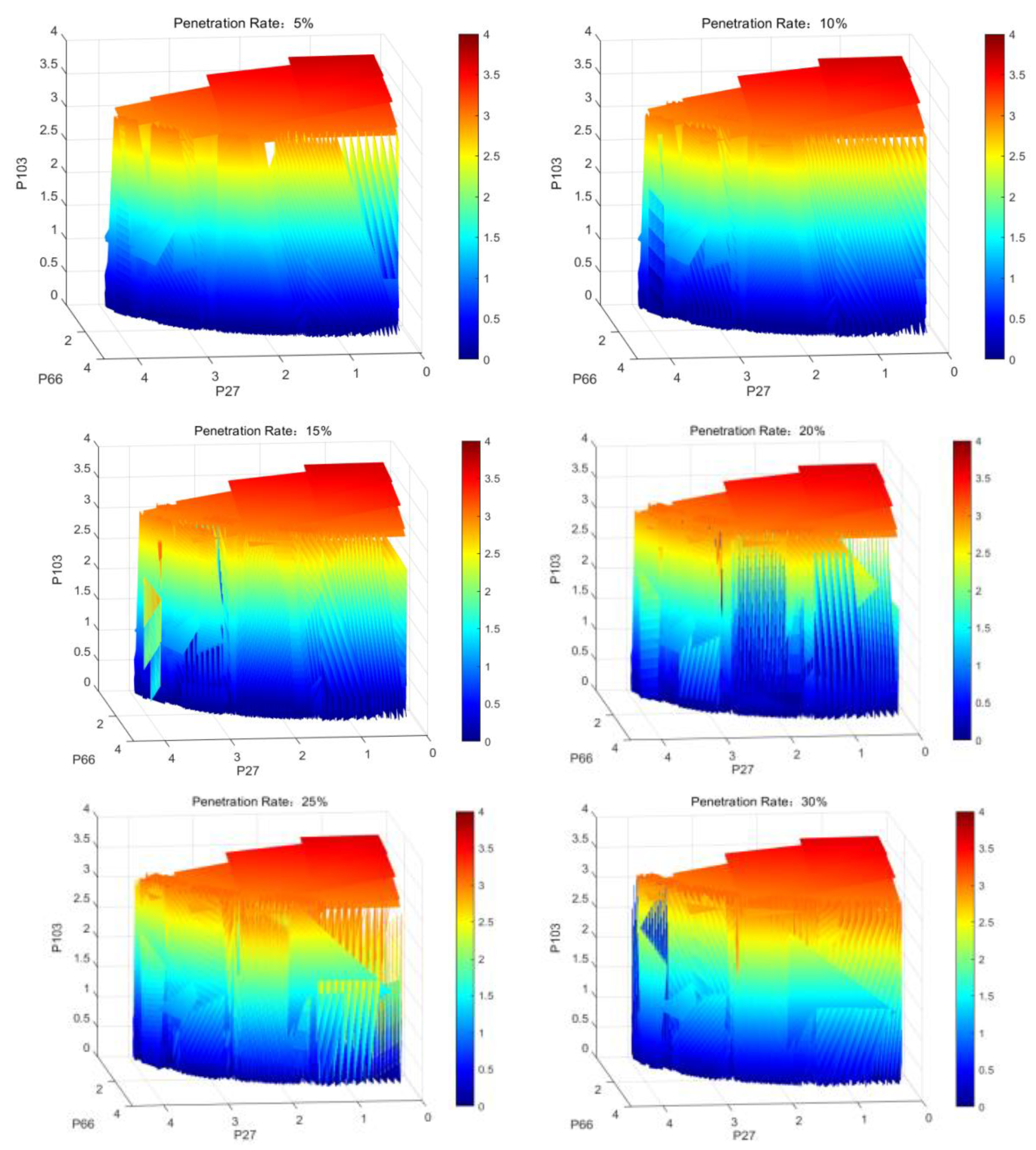
Through extensive simulation calculations, it was found that the boundary of the static security region (SSR) can be fitted using hyperplanes. Then, several operating points near the boundary are selected for time domain simulation to verify the constructed boundary, ensuring that the error remains within the permissible range for engineering applications. The figure below shows the cases where the penetration rate ranges from 5% to 50%.
The SSR constructed in three-dimensional space visually reveals the range of static security in the three-dimensional space, delineated by the coordinated active power output of synchronous units G103 and G66, along with the active power output of DFIG wind turbine D27. The SSR constructed from these three entities exhibits a smooth characteristic. As the penetration rate of new energy increases, the determining factors of the SSR boundary tend to converge towards new energy sources. The static security domain between the three entities was fitted by critical points searched using an improved gradient descent method.
In Figure 10, from the top left to the bottom right, one can observe significant changes in certain areas of the graph as the wind power penetration rate increases. At lower penetration rates, the data appear more concentrated and coherent. As the penetration rate increases, the data begin to exhibit greater fluctuations, especially in certain areas in Figure 10 at penetration rates of 45% and 50% (such as the transition area from yellow to red) where abrupt changes occur, indicating that the system behaves more dynamically or unstably at higher penetration rates.
At lower penetration rates, the system exhibits more stable behavior with a relatively even distribution of active power. As the penetration rate increases, the graph becomes more variable, particularly in areas with higher power levels. This means that as more wind power is integrated, the system becomes more dynamic and requires more regulation to maintain stability. At high penetration rates (such as 45% and 50%), the system experiences significant fluctuations, indicating potential stability issues at these nodes, which need to be addressed by adjusting the outputs of other nodes or by adding energy storage and other frequency regulation measures.
From the perspective of the safety domain, at low penetration rates, the safety domain is larger, meaning that the power system can operate safely within a larger state space. At high penetration rates, the safety domain irregularly shrinks, indicating that the system is more sensitive to power changes, with stricter operational restrictions. Particular attention is given to the static safety domain of the system with a wind power penetration rate of 40%. Although its stability is not as good as that at about 10% penetration in Figure 10, it generally meets the stability requirements.
5.3. Validation of Effectiveness
- (1)
- Validation of engineering allowable error
Taking a 40% new energy penetration rate as an example, to validate the effectiveness of the proposed method, it was compared with the traditional fitting method. The comparison was based on the error defined as the average ratio of the distance between all critical points (injection power vectors) and the boundary of the hyperplane to the magnitude of the injection power vector at that moment.
In the equation, represents the distance from the critical point to the system hyperplane, represents the module of the critical point in the system (module of the power vector), and represents the coefficients of the system hyperplane.
The comparison of errors between the method used in this article and the traditional fitting method is shown in Table 2.
Out of the 268 critical points in the three-dimensional safe region, 249 points have a relative error of less than 0.5%, accounting for 92.91% of the total; 19 points have a relative error between 0.5% and 1.5%, accounting for 7.09% of the total; and the maximum relative error is 1.365%. All errors are within the permissible engineering tolerance (5%).
- (2)
- Boundary Time Domain Validation
Taking a 40% new energy penetration rate as an example, a number of running points are found at the boundary point for time domain simulation, and then the boundary is constructed accurately based on whether the simulation result is in a stable state and whether the region where the point is located is a safe region. In order to further verify the accuracy of the result, several points near the critical surface of the safety domain are taken for time domain simulation verification.
The time domain simulation at operating points 2, 9, and 10 resulted in an unstable state, and these points are located outside the hyperplane, not satisfying the stability constraints. Based on the results of the time domain simulation in Table 3, the determination obtained through the stochastic–batch gradient descent with the gradient accumulation strategy remains consistent with the time domain simulation, indicating that the use of the improved stochastic–batch gradient descent and gradient accumulation strategy effectively searches for the SSR with the required accuracy.
5.4. Compare and Analyze the Results Obtained from Different Methods
To validate the effectiveness and accuracy of the improved stochastic–batch gradient descent algorithm, different methods before and after the improvement are compared to observe the enhancements in computational efficiency and precision achieved by the improvements to the gradient descent algorithm.
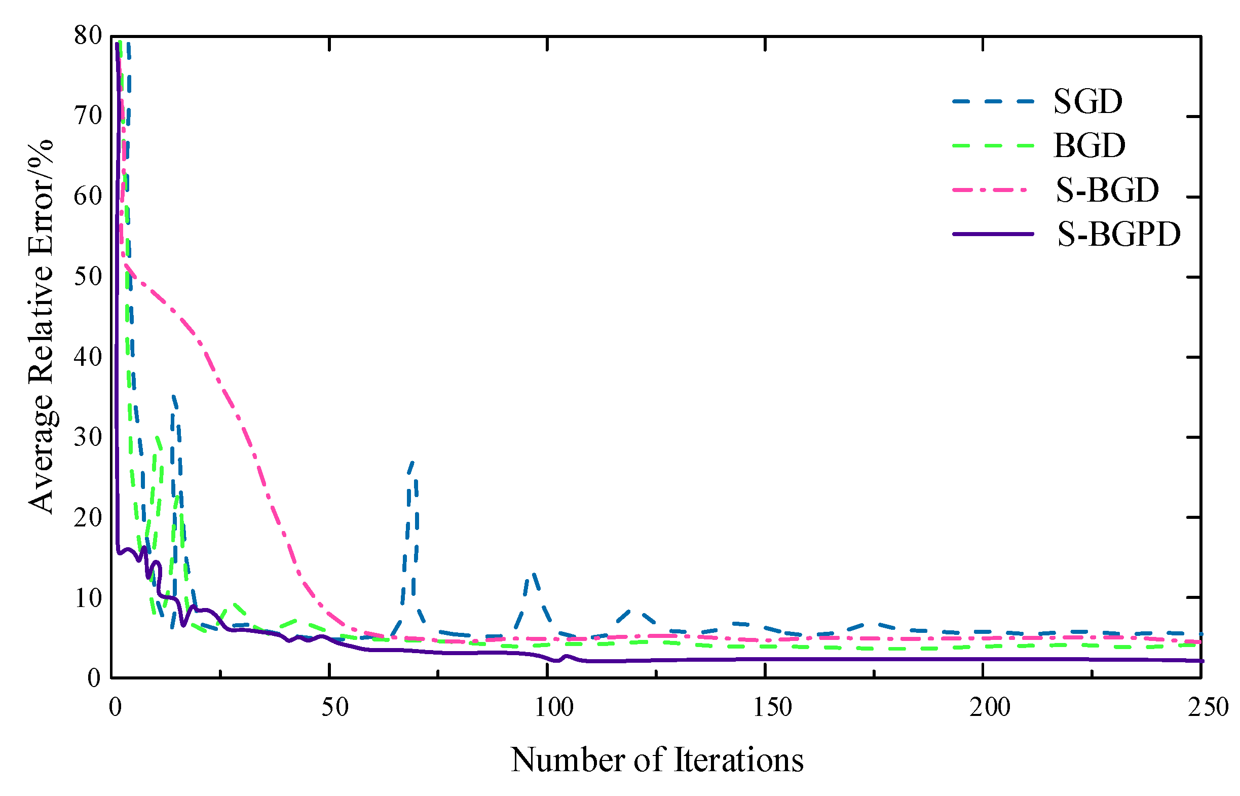
In Figure 11, it is evident that all four methods converge. BGD converges slower due to the use of a smaller step size to ensure stability. On the other hand, SGD iterates with a single sample at a time, which prevents it from exploring the global optimal solution, leading to oscillations in the convergence curve. Compared to these two methods, S-BGD demonstrates better convergence characteristics. Its convergence is more stable and efficient than BGD and SGD.
In Table 4, it can be observed that the S-BGD method has a lower fitting error compared to the SGD and BGD methods, indicating that the S-BGD method, which combines both the SGD and BGD methods, exhibits better optimization capabilities than using the SGD or BGD methods individually. Furthermore, the S-BGPD method outperforms the S-BGD method in terms of fitting accuracy, indicating that the incorporation of the gradient accumulation strategy GP allows the S-BGPD method to obtain relatively superior solutions and thereby improves fitting precision.
Regarding training time, the BGD and S-BGD methods have training times of 572.56 s and 312.42 s, respectively. This demonstrates that the S-BGD method achieves a 45% reduction in training time compared to BGD, highlighting its enhanced computational efficiency. On the other hand, the S-BGPD method has a training time of 376.59 s, representing a 20% increase compared to S-BGD. This increase in training time is mainly due to the introduction of the gradient accumulation strategy GP, which elongates the search path to avoid local optima or saddle points and increases the computational load.
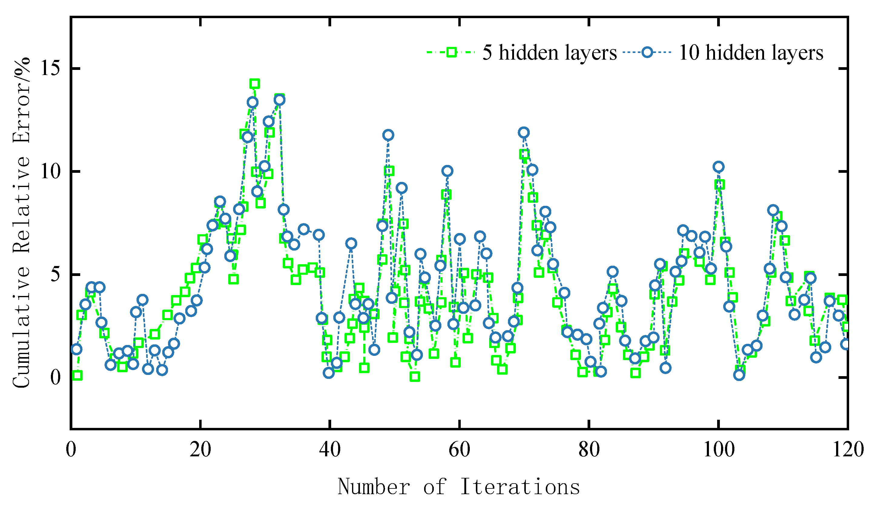
To validate the effectiveness and accuracy of the choice of hidden layers, the S-BGPD method was employed in the same IEEE-118 bus system with configurations of 5 and 10 hidden layers, respectively, to optimize and observe their error results.
In Figure 12, it can be observed that after more than 100 iterations, the cumulative relative errors of the optimization results in five and ten hidden layers that are not significantly different. It can tentatively be concluded that the results obtained using the S-BGPD method with either configuration are similar. The reason for not considering more layers is that too many layers may lead to overfitting, where the model learns the noise in the training data, leading to poor generalization of new data. Therefore, considering computational efficiency, it is advisable to choose five hidden layers.
6. Conclusions
This paper presents an improved strategy for parameter optimization training and applies it to static safety domain analysis in power systems. The proposed deep learning algorithm with the improved stochastic–batch gradient descent method is employed to construct the static safety domain in power systems under high penetration of new energy sources. This study extensively utilizes time domain simulations on the test system and finds that the boundary can be effectively approximated using the hyperplane method, displaying smooth linear characteristics and fitting errors within the acceptable engineering range. Based on the test results, the following conclusions are drawn:
(1) The combination of stochastic gradient descent (SGD) and batch gradient descent (BGD) in the training of parameters for deep learning prediction models can effectively improve both training efficiency and performance.
(2) The utilization of the gradient accumulation strategy during the training process with SGD and BGD helps to address the problem of easily getting trapped in local optima and saddle points, leading to enhanced accuracy in the model.
(3) When compared to the traditional shallow training Backpropagation (BP) neural network algorithm, the proposed deep learning approach in this paper significantly reduces the cumulative relative error and maintains consistent results with time domain simulation verification. These findings demonstrate the effectiveness of the proposed method in power system static safety domain analysis.
(4) In the IEEE-118 node system, the variation patterns of the static security domain boundaries were explored under different wind power penetration rates. From the perspective of the security domain, at low penetration rates, the security domain is larger, indicating that the power system can operate safely within a larger state space. At high penetration rates, the security domain irregularly contracts, showing that the system is more sensitive to power changes and has stricter operational restrictions. Special attention was given to the static security domain at a 40% wind power penetration rate, where the power system meets the stability requirements of high-penetration power systems.
Author Contributions
Conceptualization, J.W., Y.Z. and H.W.; methodology, J.W.; software, Y.Z. and H.W.; validation, J.W.; formal analysis, J.W.; investigation, H.W.; resources, W.W.; data curation, Y.Z.; writing—original draft preparation, J.W.; writing—review and editing, Y.Z.; visualization, Y.Z.; supervision, W.W.; project administration, H.W.; funding acquisition, J.W. All authors have read and agreed to the published version of the manuscript.
Funding
This research was funded by a project supported by the Open Project of the Key Laboratory in Xinjiang Uygur Autonomous Region of China (2023D04071) and the National Natural Science Foundation of China (52167016). This project was supported by the Key Research and Development Project of Xinjiang Uygur Autonomous Region (2022B01020-3).
Institutional Review Board Statement
Not applicable.
Informed Consent Statement
Not applicable.
Data Availability Statement
The original contributions presented in the study are included in the article, further inquiries can be directed to the corresponding author.
Conflicts of Interest
The authors declare no conflicts of interest.
Abbreviations
| SSR | Static Security Region |
| GD | Gradient Descent |
| BGD | Batch Gradient Descent |
| SGD | Stochastic Gradient Descent |
| MBGD | Mini-Batch Gradient Descent |
| S-BGD | Stochastic–Batch Gradient Descent |
| GP | Gradient Pile |
| S-BGPD | Stochastic–Batch Gradient Pile Descent |
Appendix A

Table A1.
Coefficients of the approximate three-dimensional SSR hyperplane in the IEEE-118 node system.
Table A1.
Coefficients of the approximate three-dimensional SSR hyperplane in the IEEE-118 node system.
| Hyperplane | a | b | c | d | P27 | P66 |
|---|---|---|---|---|---|---|
| 1 | −0.2019 | −1.1878 | −0.0556 | 3.3851 | [2.5200, 2.8151] | [0.1600, 1.8960] |
| 2 | -0.2688 | −0.5399 | −0.0583 | 1.8795 | [2.1271, 2.6622] | [1.4620, 2.6850] |
| 3 | −0.6484 | −0.5816 | −0.0080 | 2.9793 | [1.1796, 2.1422] | [2.6630, 3.5350] |
| 4 | −0.6976 | −0.3041 | −0.0302 | 2.8296 | [0.1600, 1.1920] | [3.5000, 3.9794] |
| 5 | −0.0827 | −0.8909 | −0.0590 | 2.5425 | [2.6622, 2.7831] | [0.1600, 1.4620] |
| 6 | −0.3558 | −0.8218 | −0.0596 | 2.7583 | [2.1422, 2.6622] | [1.4520, 2.6630] |
| 7 | −0.6502 | −0.5727 | −0.0641 | 3.0125 | [1.1920, 2.1422] | [2.6370, 3.5000] |
| 8 | −1.3144 | −0.3262 | −0.8047 | 5.9583 | [0.1600, 2.0809] | [3.2300, 3.9767] |
| 9 | −0.0827 | −0.8840 | −0.0666 | 2.5354 | [2.6169, 2.7378] | [0.1600, 1.4520] |
| 10 | −0.3570 | −0.8108 | −0.0377 | 2.6979 | [2.0951, 2.6169] | [1.4100, 2.6370] |
| 11 | −0.4203 | −0.4058 | −0.0196 | 1.9884 | [1.4809, 2.1138] | [2.5870, 3.2300] |
| 12 | −0.9038 | −0.4702 | 0.0270 | 3.5743 | [0.1600, 1.4809] | [3.2300, 3.9172] |
| 13 | −0.0566 | −0.8553 | −0.1022 | 2.5328 | [2.6036, 2.6862] | [0.1600, 1.4100] |
| 14 | −0.3351 | −0.8054 | −0.0632 | 2.7093 | [2.1138, 2.6036] | [1.3770, 2.5870] |
| 15 | −0.6429 | −0.5631 | −0.0790 | 3.0282 | [1.1742, 2.1138] | [2.5310, 3.4100] |
| 16 | −0.6940 | −0.3407 | −0.0883 | 2.9618 | [0.1600, 1.1742] | [3.3330, 3.9079] |
| 17 | −0.0280 | −0.8327 | −2.9749 | 10.7914 | [0.1600, 2.6044] | [0.1600, 1.3770] |
| 18 | −0.3297 | −0.7896 | −3.3600 | 12.2121 | [0.1600, 2.5636] | [0.1600, 2.5310] |
| 19 | −0.6350 | −0.5488 | −3.7416 | 13.5887 | [0.1600, 2.0818] | [0.1600, 3.3330] |
| 20 | −0.6800 | −0.3460 | −3.6558 | 13.2564 | [0.1600, 1.1538] | [0.1600, 3.8387] |
| 21 | 0.0827 | 0.8909 | −0.1327 | −2.3806 | [2.5200, 2.7831] | [0.1600, 1.8960] |
| 22 | 0.3558 | 0.8218 | −0.0067 | −2.7023 | [2.1271, 2.6622] | [1.4620, 2.6850] |
| 23 | 0.6502 | 0.5727 | 0.0228 | −2.9776 | [1.1796, 2.1422] | [2.6630, 3.5350] |
| 24 | 0.7061 | 0.3262 | 0.0028 | −2.8626 | [0.1600, 1.1920] | [3.5000, 3.9794] |
| 25 | 0.0827 | 0.8840 | 0.0598 | −2.5249 | [2.6169, 2.7378] | [0.1600, 1.4620] |
| 26 | 0.3570 | 0.8108 | 0.0694 | −2.7463 | [2.0951, 2.6169] | [1.4520, 2.6630] |
| 27 | 0.4203 | 0.4058 | −0.0055 | −1.9500 | [1.1920, 2.0951] | [2.6370, 3.5000] |
| 28 | 0.9038 | 0.4702 | 0.0786 | −3.7358 | [0.1600, 1.4809] | [3.2300, 3.9767] |
| 29 | 0.0566 | 0.8553 | 0.0201 | −2.3511 | [2.6036, 2.6862] | [0.1600, 1.4520] |
| 30 | 0.3351 | 0.8054 | 0.0025 | −2.5749 | [2.0951, 2.6036] | [1.4100, 2.6370] |
| 31 | 0.6429 | 0.5631 | 0.0833 | −3.0377 | [1.1742, 2.1138] | [2.5870, 3.4100] |
| 32 | 0.6940 | 0.3407 | 0.0094 | −2.7874 | [0.1600, 1.1742] | [3.4100, 3.9172] |
| 33 | 0.0280 | 0.8327 | 0.0500 | −2.3182 | [2.5636, 2.6044] | [0.1600, 1.4100] |
| 34 | 0.3297 | 0.7896 | 0.0639 | −2.6633 | [2.0818, 2.5636] | [1.3770, 2.5870] |
| 35 | 0.6350 | 0.5488 | 0.0879 | −3.0040 | [1.1538, 2.0818] | [2.5310, 3.4100] |
| 36 | 0.6800 | 0.3460 | 0.0688 | −2.8648 | [0.1600, 1.1538] | [3.3330, 3.9079] |
Appendix B
Table A2.
Formulas of iterative updating.
| Method | Variant | Formulas of Iterative Updating |
|---|---|---|
| SGD | ||
| BGD | ||
The iterative update computations for during the training processes of SGD and BGD are presented in Appendix B, as indicated.
In the table, , , and represent the weight coefficient matrix, negative gradient, and gradient accumulation of the k-th iteration, respectively. Other variables follow a similar pattern.
References
- Yan, X.; Zhang, X.; Zhang, B.; Ma, Y.; Wu, M. Research on Distributed PV Storage Virtual Synchronous Generator System and Its Static Frequency Characteristic Analysis. Appl. Sci. 2018, 8, 532. [Google Scholar] [CrossRef]
- Zheng, H.; Li, B.; Liu, D.; Yin, H.; Li, Z.; Zhang, B.; Yang, H.; Yue, H.; Zhao, G.; Cui, D. On-line evaluation index of power system static stability situation based on time-sequence trajectory characteristics of voltage vorator. Power Syst. Technol. 2021, 45, 640–648. [Google Scholar]
- Wang, Z.; Li, L.; Li, Z.; Cheng, Z. The evolution characteristics of power grid frequency probability distribution. Power Syst. Prot. Control 2021, 49, 65–73. [Google Scholar]
- Jin, W.; Zhang, S.; Li, J. Robust Planning of Distributed Generators in Active Distribution Network Considering Network Reconfiguration. Appl. Sci. 2023, 13, 7747. [Google Scholar] [CrossRef]
- Jarjis, J.; Galiana, F.D. Quantitative analysis of steady state stability in power networks. IEEE Trans. Power Appar. Syst. 1981, 100, 318–326. [Google Scholar] [CrossRef]
- Lin, W.; Jiang, H.; Yang, Z. Tie-line Security Regions in High Dimension for Renewable Accommodations. arXiv 2022, arXiv:2201.01019. [Google Scholar] [CrossRef]
- Li, X.; Zhang, L.; Jiang, T.; Chen, H.; Li, G. Generic search method of power system security domain boundary based on lagrange multiplier. Proc. CSEE 2021, 41, 5139–5153. [Google Scholar]
- Jiang, T.; Zhang, M.; Cui, X.; Li, Y.; Shi, Q. Optimization model for fast search of static voltage stability region boundary in power system. Trans. China Electrotech. Soc. 2018, 33, 4167–4179. [Google Scholar]
- Zhang, Q.; Zheng, H.; Wang, J.; Liu, X.; Qu, Y.; Bie, C. Power system static voltage stability margin calculation method based on AQ node. Power Syst. Technol. 2019, 43, 714–721. [Google Scholar]
- Xia, S.; Zhang, Q.; Hussain, S.T.; Hong, B.; Zou, W. Impacts of Integration of Wind Farms on Power System Transient Stability. Appl. Sci. 2018, 8, 1289. [Google Scholar] [CrossRef]
- Li, Y.; Li, Y.; Sun, Y. Online Static Security Assessment of Power Systems Based on Lasso Algorithm. Appl. Sci. 2018, 8, 1442. [Google Scholar] [CrossRef]
- Liu, Y.; Zhang, J. Gradient Descent Method. J. East China Inst. Technol. 1993, 2, 12–22. [Google Scholar]
- Bottou, L. Online learning and stochastic approximations. Line Learn. Neural Netw. 1998, 17, 142. [Google Scholar]
- Bengio, Y.; Lamblin, P.; Popovici, D.; Larochelle, H. Greedy layer-wise training of deep networks. Adv. Neural Inf. Process. Syst. 2006, 19. [Google Scholar]
- Guo, Y.; Song, X. Analysis and Improvement of the Gradient Descent Method. Sci. Technol. 2016, 15, 115–117. [Google Scholar]
- Jang, B.; Yoo, I.; Yook, D. Pipelined Stochastic Gradient Descent with Taylor Expansion. Appl. Sci. 2023, 13, 11730. [Google Scholar] [CrossRef]
- Liu, Y.; Cheng, Y.; Tao, Q. Individual Convergence of NAG with Biased Gradient in Non-smooth Cases. J. Softw. 2020, 31, 1051–1062. [Google Scholar]
- Xie, T.; Zhang, C.; Xu, Y. Collaborative Parameter Update Based on Average Variance Reduction of Historical Gradients. J. Electron. Inf. Technol. 2021, 43, 956–964. [Google Scholar]
- Song, J.; Zhu, Y.; Xu, B. Batch Subtraction Update Variance Reduction Gradient Descent Algorithm BSUG. Comput. Eng. Appl. 2020, 56, 117–123. [Google Scholar]
- Tan, H. Research on Fast Search Method for Static Security Domain Boundary of Power System; Northeast Electric Power University: Jilin, China, 2019. [Google Scholar]
- Yann, L.; Yoshua, B.; Geoffrey, H. Deep learning. Nature 2015, 521, 436–444. [Google Scholar]
- Thomas, W.; Helmut, B. A mathematical theory of deep convolutional neural networks for feature extraction. IEEE Trans. Inf. Theory 2018, 64, 1845–1866. [Google Scholar]
- Tong, Z.; Tanaka, G. Hybrid pooling for enhancement of generalization ability in deep convolutional neural networks. Neurocomputing 2019, 333, 76–85. [Google Scholar] [CrossRef]
- Fang, Z.; Feng, H.; Huang, S.; Zhou, D.-X. Theory of deep convolutional neural networks II: Spherical Analysis. Neural Netw. 2020, 131, 154–162. [Google Scholar] [CrossRef] [PubMed]
- Rumelhart, D.E.; Hinton, G.E.; Williams, R.J. Learning representations by back-propagating errors. In Parallel Distributed Processing: Explorations in the Microstructure of Cognition; The MIT Press: Cambridge, MA, USA, 1986; pp. 318–362. [Google Scholar]
- Chen, K. A Study of Efficient Training Algorithms to Deep Learning Models; University of Science and Technology of China: Hefei, China, 2016; pp. 4–6. [Google Scholar]
Figure 1.
The equivalent schematic diagram of wind farm integration into the grid.

Figure 2.
A conceptual illustration of the improved stochastic–batch gradient descent (S-BGD) search method.
Figure 2.
A conceptual illustration of the improved stochastic–batch gradient descent (S-BGD) search method.

Figure 3.
The search process based on gradient accumulation.

Figure 4.
Model structure.

Figure 5.
The pre-training structures for the first and second hidden layers.

Figure 6.
Flowchart for constructing security domains based on improved stochastic–batch gradient descent.
Figure 6.
Flowchart for constructing security domains based on improved stochastic–batch gradient descent.

Figure 7.
Improved IEEE 118-node test system.

Figure 8.
Two-dimensional SSR of the IEEE-118 system.

Figure 9.
The three-dimensional approximate SSR boundary of the IEEE-118 system.

Figure 10.
The SSR under new energy penetration rates ranging from 5% to 50%.


Figure 11.
Convergence curves of SGD, BGD, S-BGD, and S-BGPD.

Figure 12.
Setup of the cumulative relative error curves for different hidden layers.

Table 1.
Analytical expression for the approximate 2D SSR hyperplane of the IEEE-118 system.
| Hyperplane | Analytical Expression | Range of P27 |
|---|---|---|
| H1 | −0.1700P27-P66 + 2.8423 = 0 | [0.1600, 1.8960] |
| H2 | −0.4980P27-P66 + 3.4641 = 0 | [1.8960, 2.6850] |
| H3 | −1.1148P27-P66 + 5.1203 = 0 | [2.6850, 3.5350] |
| H4 | −2.2942P27-P66 + 9.2897 = 0 | [3.5350, 3.9794] |
Table 2.
Comparison of errors.
| Method | Penetration Rate of New Energy/% | Angle between Each Hyperplane/° | Average Fitting Error of Critical Points/% |
|---|---|---|---|
| S-BGPD | 40 | 2.12 | 1.27 |
| Traditional fitting method | 40 | 2.03 | 1.20 |
Table 3.
Time domain simulation results with a 40% penetration rate.
| Operating Point | Output of Generators G66 and G103/MW | Active Power Output of Wind Turbine D27/MW | Whether It Is Located within the Safety Domain | Time Domain Simulation |
|---|---|---|---|---|
| 1 | 2204.312297 | 1528.687703 | Yes | Stable |
| 2 | 2216.342716 | 1516.657284 | No | Unstable |
| 3 | 2239.286794 | 1493.713206 | Yes | Stable |
| 4 | 2210.594078 | 1522.405922 | Yes | Stable |
| 5 | 2206.249615 | 1526.750385 | Yes | Stable |
| 6 | 2232.481303 | 1500.518697 | Yes | Stable |
| 7 | 2169.626044 | 1563.373956 | Yes | Stable |
| 8 | 2225.400152 | 1507.599848 | Yes | Stable |
| 9 | 2227.172067 | 1505.827933 | No | Unstable |
| 10 | 2229.287542 | 1503.712458 | No | Unstable |
Table 4.
Comparison of results from different methods.
| Method | Relative Errors/% | Time/s | |
|---|---|---|---|
| Average Relative Error | Maximum Relative Error | ||
| SGD | 1.584 | 2.917 | 213.97 |
| BGD | 1.423 | 2.597 | 572.56 |
| S-BGD | 1.334 | 2.044 | 312.42 |
| S-BGPD | 1.283 | 1.419 | 376.59 |
Disclaimer/Publisher’s Note: The statements, opinions and data contained in all publications are solely those of the individual author(s) and contributor(s) and not of MDPI and/or the editor(s). MDPI and/or the editor(s) disclaim responsibility for any injury to people or property resulting from any ideas, methods, instructions or products referred to in the content. |
© 2024 by the authors. Licensee MDPI, Basel, Switzerland. This article is an open access article distributed under the terms and conditions of the Creative Commons Attribution (CC BY) license (https://creativecommons.org/licenses/by/4.0/).
Share and Cite
MDPI and ACS Style
Wu, J.; Zhou, Y.; Wang, H.; Wang, W. A Static Security Region Analysis of New Power Systems Based on Improved Stochastic–Batch Gradient Pile Descent. Appl. Sci. 2024, 14, 3730. https://doi.org/10.3390/app14093730
AMA Style
Wu J, Zhou Y, Wang H, Wang W. A Static Security Region Analysis of New Power Systems Based on Improved Stochastic–Batch Gradient Pile Descent. Applied Sciences. 2024; 14(9):3730. https://doi.org/10.3390/app14093730
Chicago/Turabian StyleWu, Jiahui, Yide Zhou, Haiyun Wang, and Weiqing Wang. 2024. "A Static Security Region Analysis of New Power Systems Based on Improved Stochastic–Batch Gradient Pile Descent" Applied Sciences 14, no. 9: 3730. https://doi.org/10.3390/app14093730
Note that from the first issue of 2016, this journal uses article numbers instead of page numbers. See further details here.