The Formation of 2D Holograms of a Noise Source and Bearing Estimation by a Vector Scalar Receiver in the High-Frequency Band

Abstract

The holographic signal-processing method for a single vector scalar receiver (VSR) in the high-frequency band in shallow water is developed in the paper. The aim of this paper is to present the results of the theoretical analysis, numerical modeling, and experimental verification of holographic signal processing for a noise source by the VSR. The developed method is based on the formation of the 2D interferogram and 2D hologram of a noise source in a shallow-water waveguide. The 2D interferograms and 2D holograms for different channels of the VSR (P sound pressure and $V_X$ and $V_Y$ vibration velocity components) are considered. It is shown that the 2D interferogram consists of parallel interference fingers in the presence of a moving noise source. As a result, the 2D hologram contains focal points located on a straight line, and the angular distribution of the holograms has the main extreme value. It is shown in the paper that the holographic signal-processing method allows detecting the source, estimating the source bearing, and filtering the useful signal from the noise. The results of the source detection, source bearing estimation, and noise filtering are presented within the framework of experimental data processing and numerical modeling.

1. Introduction

Interferometric signal processing (ISP) [1,2,3,4,5,6] is attracting considerable scientific interest in the field of underwater acoustics as a method that is an effective alternative to matched-field processing (MFP) [7,8,9,10]. ISP is based on the stable characteristics of the interference structure (pattern) of the broadband sound field in the shallow-water waveguide [1,2]. The sound field normal mode interference in underwater waveguides results in specific patterns within the sound intensity distribution, observable both in the frequency-range domain, as noted by Chuprov [1], and in the frequency-time domain, as outlined by Weston and Stevens [2]. The seminal work of Chuprov [1] laid the foundation for the mathematical theory of sound field interference in underwater acoustics. Chuprov introduced the concept of the waveguide invariant—a key factor in the analysis of interference patterns within the sound field. Notable advances in shallow-water waveguide ISP were detailed in subsequent research by Grachev and Wood [3], Orlov and Sharonov [4], Ianniello [5], and in the papers in the conference proceedings edited by Kuperman and D’Spain [6].

ISP in ocean waveguides has enabled the solution of many important problems in underwater acoustics, such as source ranging (in both passive and active modes), depth and bearing estimation, remote sensing of geo-acoustic parameters, etc. D’Spain and Kuperman [11] used the waveguide invariant for the analysis of single hydrophone spectrograms in shallow water environments. Heaney and Cox [12] proposed an incoherent method for geoacoustic characterization. Thode [13] developed the waveguide-invariant theory for source ranging with minimal environmental information and used a vertical receiving array and a guide source to construct a virtual receiver. Hodgkiss et al. [14] used the waveguide-invariant concept to move the focal point in a time-reversal experiment. Thode et al. [15] studied the sidelobe structure of a matched-field processor. Yang [16] used waveguide-invariant theory for source motion compensation. Yang [17] and Rouseff and Leigh [18] observed interference patterns in the output of a coherent processor such as a horizontal line array beamformer. Rouseff and Spindel [19] and Baggeroer [20] offered an approach for estimating invariant parameters in waveguides. In the work of Heaney [21], ISP was used to classify the seabed based on passing ship signals. In the work of Cockrell and Schmidt [22], ISP was developed to estimate the source range in shallow water. ISP was used by Rouseff and Zurk [23] for range-independent invariant estimation. The ISP approach was used by Harrison [24] to explain the interference fringes by the arrival times of the eigenrays in a waveguide. ISP was developed in the papers of Bonnel et al. [25,26] for deep-sea passive sonar. Wang and Gao [27,28,29] applied dispersion elimination technology to shallow-water acoustic signal processing and demonstrated some research achievements. Xiao-Le et al. [30] proposed an ISP method to estimate the range and depth using a single hydrophone based on the relationship of the horizontal wavenumber difference between two modes, with the waveguide invariant, for low-frequency underwater acoustic pulse signals in a range-independent shallow-water waveguide. Zhang et al. [31] proposed a method using the dispersive transform to extract the source position information from the dispersion. Lee and Makris [32,33,34] proposed the concept of the array-invariant technique. Rui Duan et al. [35] applied ISP to analyze the vertical angle of arrivals for source depth estimation. Song and Byun [36,37,38] developed an adaptive ISP method based on array invariance for source-range estimation in shallow water. Knobles et al. [39] used the ISP method to solve the geoacoustic inversion problem. Yao et al. [40] analyzed the interference pattern of a source below the critical depth in a deep-ocean waveguide. Kim et al. [41] developed an approach to estimate the source localization using the array-invariant technique. Su et al. [42] analyzed a sound field interference pattern anomaly observed in shallow water. Li et al. [43] used the interferometric method for depth estimation in shallow water with a thermocline. Pang et al. [44] developed an algorithm to extract the interference structure in the reverberation sound field. Li et al. [45] used the ISP approach to suppress tonal interference. Li et al. [46] developed an interferometric beamforming method for range estimation.

One of the most advantageous approaches of ISP is holographic signal processing (HSP) [47,48,49,50,51,52,53]. The physical and mathematical principles of hologram formation were first described by Kuz’kin and Pereselkov [47]. In the papers [48,49], HSP was analyzed for the low-frequency band in a regular waveguide. In the paper [50], the resolution of the sources by HSP was used. In the paper [51], HSP was developed for the noise source. In the papers [52,53], the HSP method was analyzed for an irregular waveguide in the presence of internal waves. The approach of HSP for sound field mode selection in a shallow-water waveguide was offered in the paper [54]. Adaptive algorithms of HSP were developed in the paper [55]. In the paper [56], HSP was used for signals from extended antennas in shallow water. In the development of HSP, it was assumed that acoustic signals from the source are recorded by hydrophones (sound pressure) in the low-frequency band. However, in many useful cases, acoustic signals are recorded by a vector scalar receiver (VSR) [57,58,59,60,61,62,63,64,65] in the high-frequency band. The VSR and the high-frequency band give us additional capabilities in solving underwater acoustics problems. First, the high-frequency band allows accumulating more sound intensity in focal points in the 2D hologram domain. Second, compared to the hydrophone, the VSR records acoustic signals on four channels: the sound pressure $P\left(t\right)$, $V_X\left(t\right)$, $V_Y\left(t\right)$, and $V_Z\left(t\right)$ components of the vibration velocities [57,58,59,60,61,62,63,64,65,66]. Horizontal components $V_X\left(t\right)$ and $V_Y\left(t\right)$ can be used for source bearing estimation. Therefore, it seems advisable to develop the HSP method for use with single VSRs in the high-frequency band.

The HSP method for a single VSR in the high-frequency band in shallow water is developed in the paper. The aim of this paper is to present the results of the theoretical analysis, numerical modeling, and experimental verification of HSP for a noise source by the VSR. The developed method is based on the formation of the 2D interferogram and 2D hologram of a noise source in a shallow-water waveguide. The 2D interferograms and 2D holograms for different channels of the VSR (P sound pressure and $V_X$ and $V_Y$ vibration velocity components) are considered. It is shown that the 2D interferogram consists of parallel interference fingers in the presence of a moving noise source. As a result, the 2D hologram contains focal points located on a straight line and the angular distribution of the holograms has the main extreme value. It is shown in the paper that the proposed HSP method allows detecting the source, estimating the source bearing, and filtering the useful signal from the noise. The results of the source detection, source bearing estimation, and noise filtering are presented within the framework of the experimental data processing and numerical modeling.

This paper is divided into five main sections. Section 1 provides a comprehensive review of the papers on ISP methods based on the waveguide-invariant technique in oceanic environments. Section 2 deals with the theory of HSP by the VSR in the high-frequency band within a shallow-water waveguide and is further divided into five subsections. Section 2.1 contains the ray description of the vector sound field (P sound pressure and $V_X$, $V_Y$, $V_Z$, and $V_R$ vibration velocity components) of a moving source in the high-frequency band. Section 2.2 introduces the HSP method for generating 2D interferograms ($I_P$, $I_X$, $I_Y$, $I_R$) in the frequency-time $(f,t)$ domain for a moving source by the VSR. Section 2.3 describes the HSP method for generating 2D holograms ($F_P$, $F_X$, $F_Y$, $F_R$) in the time-frequency $(\tau ,\nu )$ domain by 2D Fourier transform (2D FT) of 2D interferograms ($I_P$, $I_X$, $I_Y$, $I_R$). Section 2.4 presents the HSP algorithm for moving source detection using a VSR. Section 2.5 considers the HSP algorithm for estimating the bearing of the moving source using a VSR. Section 3 analyzes the 2D interferograms ($I_P$, $I_X$, $I_Y$, $I_R$), 2D holograms ($F_P$, $F_X$, $F_Y$, $F_R$), and angular hologram distributions ($G_P$, $G_X$, $G_Y$, $G_R$) and reconstructs the time dependence of the source bearing using numerical modeling. Section 4 verifies the developed HSP method by experimental data processing and analyzes the same sets: 2D interferograms ($I_P$, $I_X$, $I_Y$, $I_R$), 2D holograms ($F_P$, $F_X$, $F_Y$, $F_R$), angle hologram distributions ($G_P$, $G_X$, $G_Y$, $G_R$), and the reconstruction of the time dependence of the source bearing. In Section 4, the possibility of filtering the useful signal from the noise is also demonstrated using experimental data. Finally, Section 5 summarizes the results of the work, highlighting the main findings and contributions to ISP.

2. Holographic Method of Signal Processing in a Shallow-Water Waveguide

2.1. High-Frequency Sound Field of a Moving Source in Shallow Water

Consider the high-frequency sound field in a 3D model of a shallow-water waveguide. The vertical plane of the waveguide is shown in Figure 1. The horizontal plane of the waveguide is shown in Figure 2. The waveguide is represented in the $(X,Y,Z)$ coordinate system as a layer of water with sound speed $c(\overrightarrow{r},z)$. Here, $\overrightarrow{r}=(x,y)$ is the radius vector in the horizontal plane. The water layer is limited at depth by a free surface $(z=0)$ and the sea bottom ($z=H$). The reflection coefficient of the water-bottom boundary is W.

The VSR is at point Q: $\overrightarrow{r_r}(x_r,y_r,z_r)$. The high-frequency sound source moves to point S: $\overrightarrow{r_s}(x_s\left(t\right),y_s\left(t\right),z_s\left(t\right))$. Here, $\overrightarrow{r_s}\left(t\right)=\overrightarrow{r_0}+\overrightarrow{v}t$, where $\overrightarrow{v}$ is the source velocity. The spectrum of the signal emitted by the source is $s\left(\omega \right)$, where $\omega =2\pi f$ is the sound frequency.

Let us consider the sound field using the method of image sources [67,68]. In the waveguide, the sound field is multi-reflected between the two boundaries. Each reflection of a sound ray from a waveguide boundary requires the inclusion of an image source in the total sound field at the receiver point. Figure 1 shows a schematic representation of the contributions from the physical source at depth $z_s$ and the first two image sources, leading to the first three terms in the expression of the total sound field. Each free surface reflection of a ray results in a multiplier $(-1)$ in the corresponding term. Each bottom reflection results in a multiplier W in the corresponding term. The total complex sound pressure at point Q can be written as an infinite sum of the fourth terms [67,68] in the following way:

$$\begin{array}{c}P(r\left(t\right),z_s,z_r,\omega )=-\frac{s\left(\omega \right)}{4\pi }\sum _{m=0}^{\infty }{(-W)}^m[\frac{exp\left(\mathrm{i}k\left(\omega \right)r_{m0}\right)}{r_{m0}}+W\frac{exp\left(\mathrm{i}k\left(\omega \right)r_{m1}\right)}{r_{m1}}+\hfill \\ \hfill -\frac{exp\left(\mathrm{i}k\left(\omega \right)r_{m2}\right)}{r_{m2}}-W\frac{exp\left(\mathrm{i}k\left(\omega \right)r_{m3}\right)}{r_{m3}}],\end{array}$$

(1)

where $r\left(t\right)=|{\overrightarrow{r}}_r-{\overrightarrow{r}}_s\left(t\right)|$ is the range between the source and VSR and $k\left(\omega \right)=\omega /c$ is the sound wavenumber. Here,

$$r_{mj}={\left(r^2\left(t\right)+z_{mj}^2\right)}^{1/2},$$

(2)

where the values $z_{mj}$ are defined as follows:

$$\begin{array}{cc}\hfill z_{m0}=2Hm+z_s-z_r;z_{m1}=2H(m+1)-z_s-z_r;& \\ \hfill z_{m2}=2Hm+z_s+z_r;z_{m3}=2H(m+1)-z_s+z_r;& \\ \hfill m=0,1,2,\dots ;& j=0,1,2,3.\hfill \end{array}$$

(3)

Consider the VSR, which consists of three accelerometers and a scalar hydrophone. The scalar hydrophone of the VSR allows measuring the sound pressure P. The three accelerometers of the VSR allow measuring three components of the vibration acceleration (particle acceleration), $\mathbf{A}=(A_X,A_Y,A_Z)$. The complex field of vibration acceleration $\mathbf{A}$ can be expressed by Euler’s equation [57] as follows:

$$\mathbf{A}=-\frac{1}{\rho }\nabla P.$$

(4)

From Equation (4), the expressions for the horizontal acceleration components $A_X$ and $A_Y$ can be obtained by differentiating Equation (1):

$$\begin{array}{cc}\hfill & A_X\left(r\left(t\right),z_s,z_r,\omega \right)=-\frac{1}{\rho }\frac{\partial P}{\partial x}=\hfill \\ \hfill & =\frac{s\left(\omega \right)}{4\pi }\frac{r}{\rho }\sum _{m=0}^{\infty }{(-W)}^m[\frac{exp\left(\mathrm{i}k\left(\omega \right)r_{m0}\right)\left(\mathrm{i}k{r}_{m0}-1\right)}{r_{m0}^3}+W\frac{exp\left(\mathrm{i}k\left(\omega \right)r_{m1}\right)\left(\mathrm{i}k{r}_{m1}-1\right)}{r_{m1}^3}\hfill \\ \hfill & -\frac{exp\left(\mathrm{i}k\left(\omega \right)r_{m2}\right)\left(\mathrm{i}k{r}_{m2}-1\right)}{r_{m2}^3}-W\frac{exp\left(\mathrm{i}k\left(\omega \right)r_{m3}\right)\left(\mathrm{i}k{r}_{m3}-1\right)}{r_{m3}^3}]\frac{\partial r}{\partial x},\hfill \end{array}$$

(5)

$$\begin{array}{cc}\hfill & A_Y\left(r\left(t\right),z_s,z_r,\omega \right)=-\frac{1}{\rho }\frac{\partial P}{\partial y}=\hfill \\ \hfill & =\frac{s\left(\omega \right)}{4\pi }\frac{r}{\rho }\sum _{m=0}^{\infty }{(-W)}^m[\frac{exp\left(\mathrm{i}k\left(\omega \right)r_{m0}\right)\left(\mathrm{i}k{r}_{m0}-1\right)}{r_{m0}^3}+W\frac{exp\left(\mathrm{i}k\left(\omega \right)r_{m1}\right)\left(\mathrm{i}k{r}_{m1}-1\right)}{r_{m1}^3}\hfill \\ \hfill & -\frac{exp\left(\mathrm{i}k\left(\omega \right)r_{m2}\right)\left(\mathrm{i}k{r}_{m2}-1\right)}{r_{m2}^3}-W\frac{exp\left(\mathrm{i}k\left(\omega \right)r_{m3}\right)\left(\mathrm{i}k{r}_{m3}-1\right)}{r_{m3}^3}]\frac{\partial r}{\partial y}.\hfill \end{array}$$

(6)

The vibration velocity (particle velocity) $\mathbf{V}=(V_X,V_Y,V_Z)$ is the integral of the acceleration in the time domain [57]. As a result of the integration of Equation (4):

$$\mathbf{V}=\frac{\mathrm{i}}{\omega }\mathbf{A}=-\frac{\mathrm{i}}{\omega \rho }\nabla P.$$

(7)

From Equation (5), Equation (6), and Equation (7), the expressions for the horizontal velocity components $V_X,V_Y,$ can be obtained as follows:

$$\begin{array}{cc}\hfill & V_X\left(r\left(t\right),z_s,z_r,\omega \right)=\frac{\mathrm{i}}{\omega }{A}_X=\hfill \\ \hfill & =\frac{s\left(\omega \right)}{4\pi }\frac{\mathrm{i}r}{\omega \rho }\sum _{m=0}^{\infty }{(-W)}^m[\frac{exp\left(\mathrm{i}k\left(\omega \right)r_{m0}\right)\left(\mathrm{i}k{r}_{m0}-1\right)}{r_{m0}^3}+W\frac{exp\left(\mathrm{i}k\left(\omega \right)r_{m1}\right)\left(\mathrm{i}k{r}_{m1}-1\right)}{r_{m1}^3}\hfill \\ \hfill & -\frac{exp\left(\mathrm{i}k\left(\omega \right)r_{m2}\right)\left(\mathrm{i}k{r}_{m2}-1\right)}{r_{m2}^3}-W\frac{exp\left(\mathrm{i}k\left(\omega \right)r_{m3}\right)\left(\mathrm{i}k{r}_{m3}-1\right)}{r_{m3}^3}]\frac{\partial r}{\partial x},\hfill \end{array}$$

(8)

$$\begin{array}{cc}\hfill & V_Y(r\left(t\right),z_s,z_r,\omega )=\frac{\mathrm{i}}{\omega }{A}_Y=\hfill \\ \hfill & =\frac{s\left(\omega \right)}{4\pi }\frac{\mathrm{i}r}{\omega \rho }\sum _{m=0}^{\infty }{(-W)}^m[\frac{exp\left(\mathrm{i}k\left(\omega \right)r_{m0}\right)\left(\mathrm{i}k{r}_{m0}-1\right)}{r_{m0}^3}+W\frac{exp\left(\mathrm{i}k\left(\omega \right)r_{m1}\right)\left(\mathrm{i}k{r}_{m1}-1\right)}{r_{m1}^3}\hfill \\ \hfill & -\frac{exp\left(\mathrm{i}k\left(\omega \right)r_{m2}\right)\left(\mathrm{i}k{r}_{m2}-1\right)}{r_{m2}^3}-W\frac{exp\left(\mathrm{i}k\left(\omega \right)r_{m3}\right)\left(\mathrm{i}k{r}_{m3}-1\right)}{r_{m3}^3}]\frac{\partial r}{\partial y}.\hfill \end{array}$$

(9)

Taking into account $\partial r/\partial x=cos\varphi$, $\partial r/\partial y=sin\varphi$, we can simplify Equations (8) and (9):

$$V_X=V_{R}cos\varphi ,V_Y=V_{R}sin\varphi ,$$

(10)

where $\varphi$ is the source bearing and $V_R$ is the vibration velocity complex field in the horizontal plane:

$$\begin{array}{cc}\hfill & V_R\left(r\left(t\right),z_s,z_r,\omega \right)=\hfill \\ \hfill & =\frac{s\left(\omega \right)}{4\pi }\frac{\mathrm{i}r}{\omega \rho }\sum _{m=0}^{\infty }{(-W)}^m[\frac{exp\left(\mathrm{i}k\left(\omega \right)r_{m0}\right)\left(\mathrm{i}k{r}_{m0}-1\right)}{r_{m0}^3}+W\frac{exp\left(\mathrm{i}k\left(\omega \right)r_{m1}\right)\left(\mathrm{i}k{r}_{m1}-1\right)}{r_{m1}^3}\hfill \\ \hfill & -\frac{exp\left(\mathrm{i}k\left(\omega \right)r_{m2}\right)\left(\mathrm{i}k{r}_{m2}-1\right)}{r_{m2}^3}-W\frac{exp\left(\mathrm{i}k\left(\omega \right)r_{m3}\right)\left(\mathrm{i}k{r}_{m3}-1\right)}{r_{m3}^3}].\hfill \end{array}$$

(11)

In the remainder of this paper, we will use the following notation for the sound pressure $P(f,t)$, and the horizontal components of the vibration velocity $V_X(f,t)$, $V_Y(f,t)$, $V_R(f,t)$:

$$\begin{array}{cc}\hfill P(f,t)& =P(r\left(t\right),z_s,z_r,\omega ),\hfill \\ \hfill V_X(f,t)& =V_X(r\left(t\right),z_s,z_r,\omega ),\hfill \\ \hfill V_Y(f,t)& =V_Y(r\left(t\right),z_s,z_r,\omega ),\hfill \\ \hfill V_R(f,t)& =V_R(r\left(t\right),z_s,z_r,\omega ).\hfill \end{array}$$

(12)

2.2. The 2D Interferograms of the Moving Source Formed by a Vector Scalar Receiver

In the frequency-time variables $(f,t)$, we introduce the notation for the interferograms:

$$\begin{array}{cc}\hfill I_P(f,t)& =P(f,t)P^{*}(f,t),\hfill \\ \hfill I_X(f,t)& =V_X(f,t)V_R^{*}(f,t),\hfill \\ \hfill I_Y(f,t)& =V_Y(f,t)V_R^{*}(f,t),\hfill \\ \hfill I_R(f,t)& =V_R(f,t)V_R^{*}(f,t).\hfill \end{array}$$

(13)

The superscript asterisk indicates complex conjugation. Here, $I_P(f,t)$ is the sound pressure interferogram. $I_X(f,t)$, $I_Y(f,t)$, and $I_R(f,t)$ are the interferograms of the horizontal components of the vibration velocities. The 2D interferograms are generated in the rectangular domain $(f,t)$: $0\le t\le \Delta t$, $f_1\le f\le f_2$. Here, $\Delta t$ is the observation time; $f_{1,2}=f_0\mp (\Delta f/2)$, where $f_0$ is the mean frequency and $\Delta f$ is the frequency bandwidth. To generate the 2D interferograms, we need J samples of the source noise. The number of samples J is determined by the equation:

$$J=\frac{\Delta t}{\delta t_1+\delta t_2},$$

(14)

where $\delta t_1$ and $\delta t_2$ are the duration of the signal realizations and the time interval between them. The realizations are independent if $\delta t_2>2\pi ⁄\Delta \omega$.

The interferogram of the sound pressure $I_P(f,t)$ was analyzed in detail in the papers [48,49]. The interferograms of the horizontal components of the vibration velocities $I_X(f,t)$, $I_Y(f,t)$, and $I_R(f,t)$ have the same structure and characteristics. Thus, the method for characterizing the sound pressure interferogram described in [48,49] is applicable to the analysis of the vibration velocity interferograms. The direction of motion of the noise source can be determined from the slope of the interference fringes in the interferogram domain. If the noise source is moving toward the VSR, the slope of the interference fringes has a negative value $\delta f/\delta t<0$. If the noise source is moving away from the VSR, the slope of the interference fringes has a positive value $\delta f/\delta t>0$. If the noise source is moving at the intersection point of the VSR, the interference fringes are parallel with the time f-axis in the interferogram domain.

2.3. The 2D Holograms of the Moving Source Formed by a Vector Scalar Receiver

In holographic signal processing, the quasi-coherent accumulation of the intensity distributions $I_P(f,t)$, $I_X(f,t)$, $I_Y(f,t)$, and $I_R(f,t)$ is performed in the frequency-time domain [48,49]. The 2D Fourier transform (2D FT) is applied to the accumulated intensity of the interferograms $I(f,t)$. The result of the 2D FT of the interferogram $I(f,t)$ is called the Fourier hologram (hologram) $F(\tau ,\nu )$. The hologram $F(\tau ,\nu )$ allows concentrating the intensity of $I(f,t)$ in the focal points of the hologram domain due to the interference fingers of the interferograms.

Consider the 2D holograms of the sound pressure and horizontal components of the vibration velocities:

$$\begin{array}{cc}\hfill F_P(\tau ,\nu )& ={\int }_0^{\Delta t}{\int }_{f_1}^{f_2}{I}_P(f,t)exp\left[\mathrm{i}2\pi (\nu t-f\tau )\right]dtdf,\hfill \\ \hfill F_X(\tau ,\nu )& ={\int }_0^{\Delta t}{\int }_{f_1}^{f_2}{I}_X(f,t)exp\left[\mathrm{i}2\pi (\nu t-f\tau )\right]dtdf,\hfill \\ \hfill F_Y(\tau ,\nu )& ={\int }_0^{\Delta t}{\int }_{f_1}^{f_2}{I}_Y(f,t)exp\left[\mathrm{i}2\pi (\nu t-f\tau )\right]dtdf,\hfill \\ \hfill F_R(\tau ,\nu )& ={\int }_0^{\Delta t}{\int }_{f_1}^{f_2}{I}_R(f,t)exp\left[\mathrm{i}2\pi (\nu t-f\tau )\right]dtdf.\hfill \end{array}$$

(15)

Here, $\nu$ and $\tau$ are the frequency and time of the hologram domain; $\Delta t$ is the observation time; $f_{1,2}=f_0\mp (\Delta f/2)$, and $f_0$ and $\Delta f$ are the average frequency and spectrum width; the initial time $t=0$.

The spectral density of the hologram $F(\tau ,\nu )$ is localized in focal points, mirrored with respect to the origin [48,49]. They are in the first and third quadrants when the source moves to the receiver $(v<0)$. They are in the second and fourth quadrants when the source is moving away from the receiver $(v>0)$. Focal points located in the first and fourth quadrants are the real image of the source and, in the second and third quadrants, are a virtual image. The spectral density of the hologram $F(\tau ,\nu )$ is concentrated mainly in the band bounded by straight lines [48,49]:

$$\nu =\tilde{\epsilon }\tau +\delta \nu ,\nu =\tilde{\epsilon }\tau -\delta \nu ,$$

(16)

where $\delta \nu =1/\Delta t$ is the half-width of the focal points in the direction of the axis $\nu$ and $\tilde{\epsilon }$ is the angular coefficient of the line on which the coordinates of the focal points are located. In the direction of the axis, the half-width of the focal spots is $\delta \tau =1/\Delta f$. Outside this band, the spectral density of the hologram is practically suppressed. The angular coefficients of the interference fringes $\delta f⁄\delta t$ are given by the expression:

$$\tilde{\epsilon }=-\frac{\delta f}{\delta t},$$

(17)

where $\delta f$ is the frequency shift of the wave field maximum over time $\delta t$.

2.4. Detection of the Moving Source

Consider the angular distribution of the spectral density of the holograms $F_P(f,t)$, $F_X(f,t)$, $F_Y(f,t)$, and $F_R(f,t)$:

$$\begin{array}{cc}\hfill G_P\left(\chi \right)& ={\int }_0^{\Delta \tau }\left|F_P(\tau ,\chi \tau )\right|d\tau ,\hfill \\ \hfill G_X\left(\chi \right)& ={\int }_0^{\Delta \tau }\left|F_X(\tau ,\chi \tau )\right|d\tau ,\hfill \\ \hfill G_Y\left(\chi \right)& ={\int }_0^{\Delta \tau }\left|F_Y(\tau ,\chi \tau )\right|d\tau ,\hfill \\ \hfill G_R\left(\chi \right)& ={\int }_0^{\Delta \tau }\left|F_R(\tau ,\chi \tau )\right|d\tau ,\hfill \end{array}$$

(18)

The function $G\left(\chi \right)$ has its maximum value at $\chi =\tilde{\epsilon }$ if the source is present. The maximum value of $G\left(\tilde{\epsilon }\right)$ is two- or more times higher than the values in the other directions ($\chi \ne \tilde{\epsilon }$):

$$G\left(\tilde{\epsilon }\right)\ge 2G\left(\chi \right).$$

(19)

Equation (19) is the criterion for source detection:

• If this condition is satisfied, the source is in the waveguide;
• If the condition is not satisfied, the source is absent.

Here, $\Delta \tau$ is the linear size of the focal point along the $\tau$-axis; $\chi$ is the angular coefficient of the straight lines $\nu =\chi \tau$ in the hologram domain. Information about the transfer function of the medium is not required. If the criterion Equation (19) is fulfilled, the estimates of the moving source parameters (bearing, radial velocity, range, depth) in holographic signal processing are close to the true values [48,49].

2.5. Source Bearing Estimation

Let us consider the method of source bearing estimation. The holograms $F_X$ and $F_Y$ up to the factors $cos\varphi$ and $sin\varphi$ reproduce the hologram $F_R$, where $\varphi$ is the source bearing (Figure 2)—the angle in the horizontal plane between the axis X of the VSR and the direction to the source. Therefore,

$$|tan\varphi |=\frac{G_Y\left(\tilde{\epsilon }\right)}{G_X\left(\tilde{\epsilon }\right)}.$$

(20)

The determination of the direction to the source is ambiguous: the bearings $\pm \varphi$ and $\pi \pm \varphi$ are indistinguishable. The inverse 2D Fourier transform is used to recover the interferograms $I_X$, $I_Y$, and $I_R$. The ambiguity of the bearing is removed by determining the sign of the ratio of the interferograms:

$$\frac{I_X(f,t)}{I_R(f,t)}={\gamma }_X,\frac{I_Y(f,t)}{I_R(f,t)}={\gamma }_Y.$$

(21)

The criterion for unambiguous source bearing estimation is as follows:

• If ${\gamma }_X>0$, ${\gamma }_Y>0$, then the source is located in the first quadrant of the VSR;
• If ${\gamma }_X<0$, ${\gamma }_Y>0$, then the source is located in the second quadrant of the VSR;
• If ${\gamma }_X<0$, ${\gamma }_Y<0$, then the source is located in the third quadrant of the VSR;
• If ${\gamma }_X>0$, ${\gamma }_Y<0$, then the source is located in the fourth quadrant of the VSR.

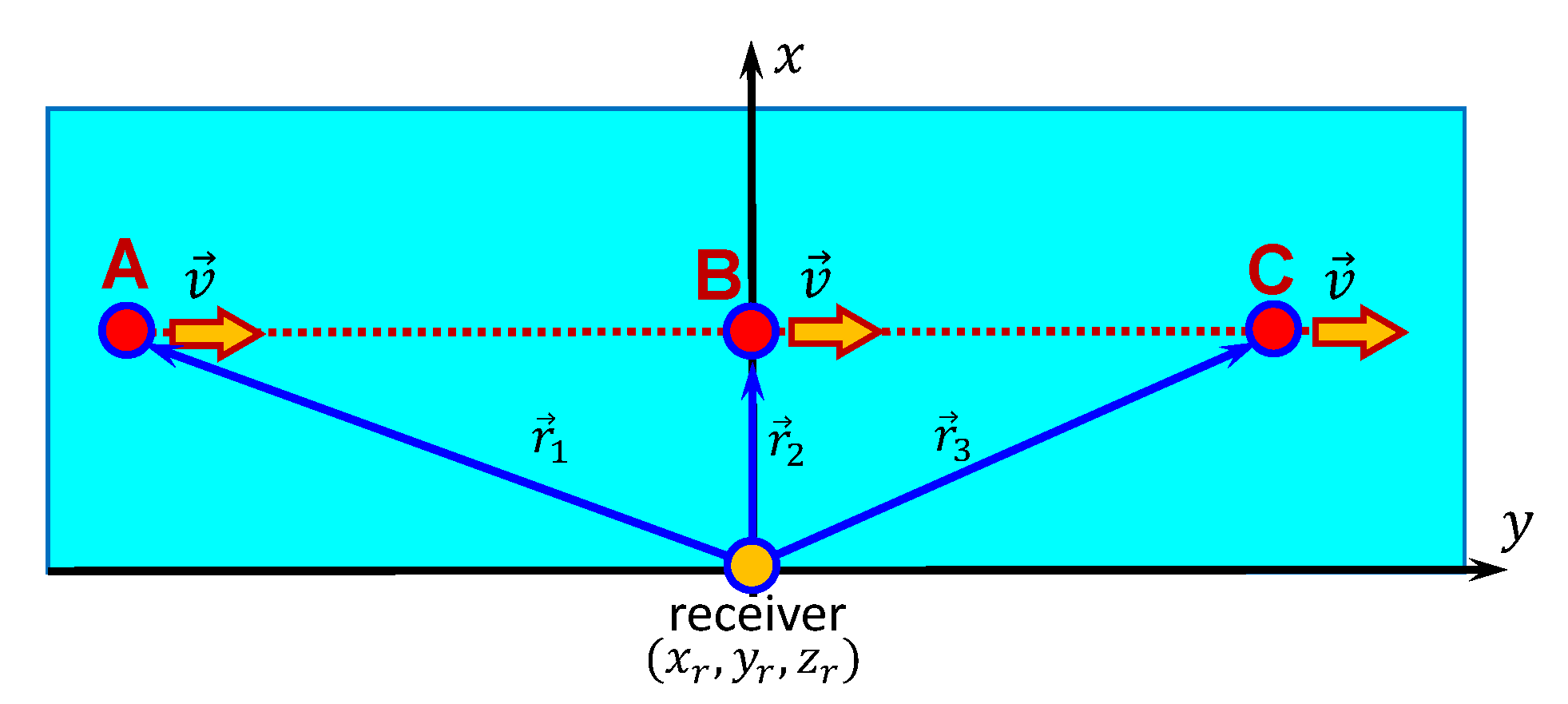
3. Numerical Simulation Results

Let us consider the following model of the shallow-water waveguide, which is close to the experimental waveguide. The vertical plane of the waveguide is shown in Figure 3. The depth of the waveguide is $H=15$ m. The sound velocity profile of the water layer is constant: $c_w\left(z\right)=1400$ m/s. The parameters of the liquid absorbing bottom are sound velocity $c_b=1780$ m/s and density ${\rho }_b=2.0$ g/cm³. The sound source at a depth of $z_s=5$ m moves along the trajectory shown in Figure 4. The source speed is $v=1.5$ m/s. The high-frequency band is $\Delta f=9$ kHz (2.5–11.5 kHz). The receiver is located at a point at a depth of $z_q=15$ m.

The trajectory of the noise source in the horizontal plane of the waveguide is shown in Figure 4. The source moves along a straight line (A→B→C), which is parallel with the y-axis.

The source trajectory parameters are as follows:

• The receiver is located at point: ($x_r=0$ m, $y_r=0$ m, $z_r=15$ m);
• The source velocity: $v=1.5$ m/s;
• The motion time: $\Delta t$ = 0–15 min;
• The motion starting point: A ($x_s=150$ m, $y_s=-675$ m, $z_s=5$ m), $r_1=691.5$ m;
• The motion traverse point: B ($x_s=150$ m, $y_s=0$ m, $z_r=5$ m), $r_2=150$ m;
• The motion finish point: C ($x_s=150$ m, $y_s=675$ m, $z_r=5$ m), $r_3=691.5$ m.

The time dependence of the coordinate $y_s\left(t\right)$ is:

$$y_s\left(t\right)=-675+1.5t.$$

The time dependence of the range $r_s\left(t\right)$ between the source and receiver is:

$$r_s\left(t\right)=\sqrt{{\left(150\right)}^2+{(-675+1.5t)}^2}.$$

The results of the numerical modeling are shown in Figure 5, Figure 6, Figure 7, Figure 8, Figure 9 and Figure 10. The interferogram of the sound pressure $I_P(f,t)$ for the time of motion $\Delta t$ = 0–15 min and, in the frequency band, $\Delta f$ = 2.5–11.5 kHz, as shown in Figure 5. The interferogram $I_P(f,t)$, hologram $F_P(\tau ,\nu )$, and angular distribution $G_P\left(\chi \right)$ for different cases of source motion are shown in Figure 6, Figure 7, Figure 8 and Figure 9.

Let us consider the results of the numerical modeling of the interferogram $I_P(f,t)$ for a source moving along the trajectory A→B→C (Figure 5) in the time-frequency domain. It can be seen that the interferogram of the sound pressure $I_P(f,t)$ has a quasi-periodic structure ($T_f$ is the period in the frequency domain). If the source moves from point A to point B, the interferogram period decreases from $T_f=9$ kHz to $T_f=1.8$ kHz. The slope of the interference fringes is negative: $\delta f⁄\delta t=-1.5$ kHz/min. When the source passes through the traverse zone, the interferogram period is $T_f=1.8$ kHz. The interference fringes are parallel to the t-axis. The result is $\delta f⁄\delta t=0$ kHz/min. As the source moves from point B to point C, the interferogram period increases from $T_f=1.8$ kHz to $T_f=9$ kHz. The slope of the interference fringes is positive: $\delta f⁄\delta t=+1.5$ kHz/min.

The interferogram $I_P(f,t)$, the hologram $F_P(\tau ,\nu )$, and the angular distribution $G_P\left(\chi \right)$ for the three cases of source motion are shown in Figure 6, Figure 7, Figure 8 and Figure 9.

$I_P(f,t)$, $F_P(\tau ,\nu )$, and $G_P\left(\chi \right)$ for the case of the source moving from point A to point B in the time interval $\Delta t=$2.5–4.2 min are shown in Figure 6. It can be seen that the slope of the interference fringes is negative: $\delta f⁄\delta t=-1.5$ kHz/min on the interferogram (Figure 6a). As a result, the focal points lie on a straight line $\nu =\tilde{\epsilon }\tau$ with an angular coefficient $\tilde{\epsilon }=40$ Hz/s in the hologram $F_P(\tau ,\nu )$ domain (Figure 6b). The angular distribution $G_P\left(\chi \right)$ has an extreme value at the point $\chi \approx -0.025$ s⁻² (Figure 6c).

$I_P(f,t)$, $F_P(\tau ,\nu )$, and $G_P\left(\chi \right)$ for the case of the source moving at point B (traverse) in the time interval Δt = 6.7–8.4 min are shown in Figure 7. It can be seen that the slope of the interference fringes is approximately zero. $\delta f⁄\delta t=0$ kHz/min on the interferogram (Figure 7a). As a result, the focal points are located at points on a straight line $\nu =\tilde{\epsilon }\tau$ with an angular coefficient of $\tilde{\epsilon }=0$ Hz/s in the hologram $F_P(\tau ,\nu )$ domain (Figure 7b). The angular distribution $G_P\left(\chi \right)$ has an extreme value at the point $\chi \approx 0$ s⁻² (Figure 7c).

$I_P(f,t)$, $F_P(\tau ,\nu )$, and $G_P\left(\chi \right)$ for the case of the source moving from point B to point C in the time interval $\Delta t=$ 10.8–12.5 min are shown in Figure 8. It can be seen that the slope of the interference fringes is negative. $\delta f⁄\delta t=+1.5$ kHz/min on the interferogram (Figure 8a). As a result, the focal points are on points on a straight line $\nu =\tilde{\epsilon }\tau$ with an angular coefficient of $\tilde{\epsilon }=-40$ Hz/s in the domain of the hologram $F_P(\tau ,\nu )$ (Figure 8b). The angular distribution $G_P\left(\chi \right)$ has an extreme value at the point $\chi \approx =+0.025$ s⁻² (Figure 8c).

The structures of the interferograms $I_X(f,t)$, $I_Y(f,t)$, and $I_R(f,t)$, holograms $F_X(\tau ,\nu )$, $F_Y(\tau ,\nu )$, and $F_R(\tau ,\nu )$, and their angular distributions $G_X\left(\chi \right)$, $G_Y\left(\chi \right)$, and $G_R\left(\chi \right)$ are the same as shown in Figure 6, Figure 7 and Figure 8:

• The interferograms $I_X$, $I_Y$, and $I_R$ have the same slope of the interference fringes as $I_P$;
• The focal points are on the same straight line $\nu =\tilde{\epsilon }\tau$ with the same angular coefficients in the hologram domain of $F_X$, $F_Y$, and $F_R$ as in the hologram domain of $F_P$;
• The angular distributions of the holograms $G_X$, $G_Y$, and $G_R$ have an extreme value at the same points.

The angular distributions of the holograms $G_X$ and $G_Y$ for three cases of source motion ($\Delta t=$ 2.5–4.2 min; $\Delta t=$ 6.7–8.4 min; $\Delta t=$ 10.8–12.5 min) are shown in Figure 9. It can be seen that the shapes of $G_X$ and $G_Y$ are the same, but the extreme values are different. For the time interval $\Delta t=$ 2.5–4.2 min, $G_Y\left({\chi }_{\max }\right)/G_X\left({\chi }_{\max }\right)\approx 2.5$. This value of $\left|\tan \varphi \right|$ corresponds to $\varphi \approx -{68}^{\circ }$. For the time interval $\Delta t=$ 6.7–8.4 min, $G_Y\left({\chi }_{\max }\right)/G_X\left({\chi }_{\max }\right)\approx 0$. This value of $\left|\tan \varphi \right|$ corresponds to $\varphi \approx 0^{\circ }$. For the time interval $\Delta t=$ 10.8–12.5 min, $G_Y\left({\chi }_{\max }\right)/G_X\left({\chi }_{\max }\right)\approx 2.5$. This value of $\left|\tan \varphi \right|$ corresponds to $\varphi \approx +{68}^{\circ }$.

Using Equation (20) $|tan\varphi |=G_Y\left({\chi }_{\max }\right)/G_X\left({\chi }_{\max }\right)$ and Equation (21), the time dependence of the source bearing $\varphi \left(t\right)$ can be calculated. The source bearing $\varphi \left(t\right)$ reconstructed by numerical modeling for the time interval $\Delta t=$ 0–15 min is shown in Figure 10. The blue solid line is the source bearing corresponding to the trajectory geometry. The red dots are the source bearings reconstructed by holographic signal processing. It can be seen that the source bearing values reconstructed within the numerical simulation are close to the true values.

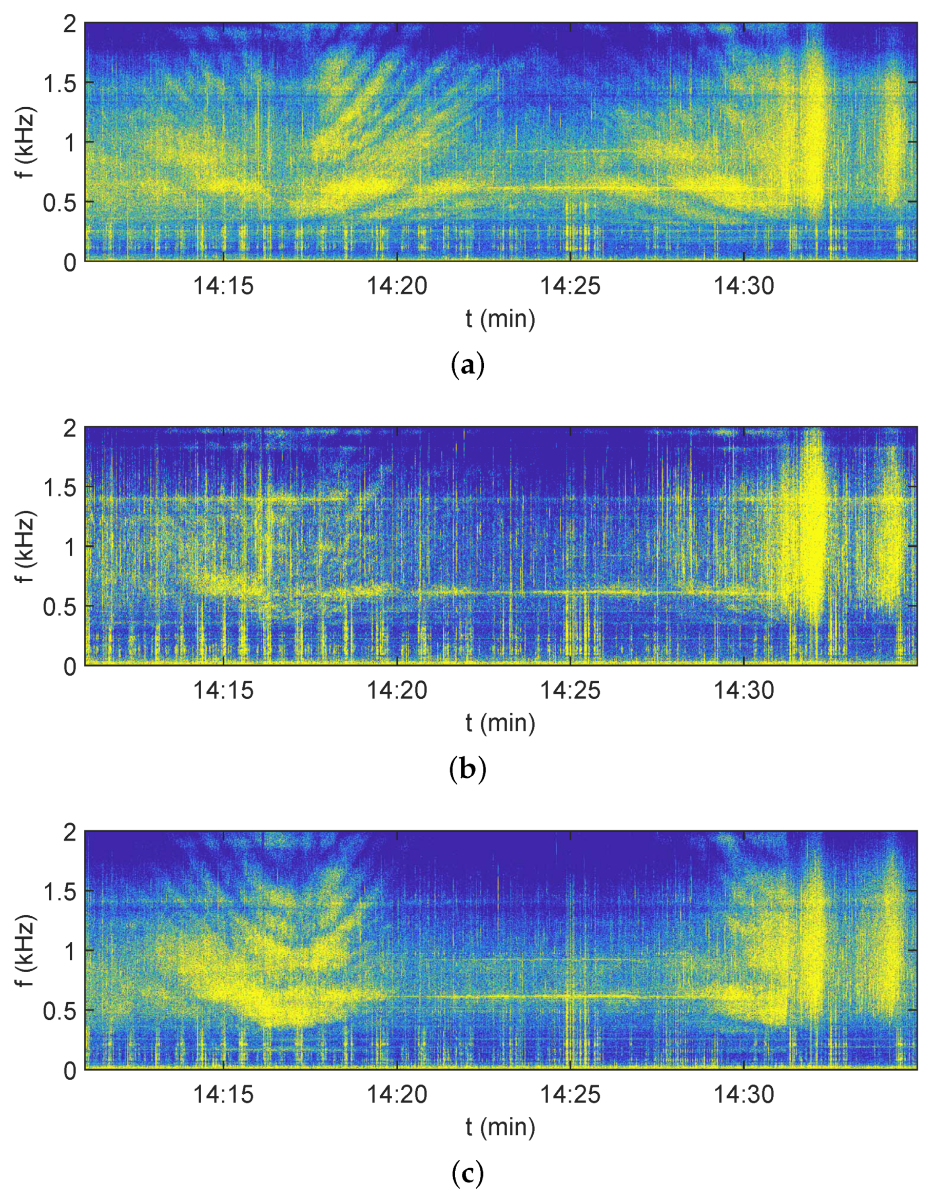
4. Experimental Results

Let us consider the experimental results of holographic signal processing in the high-frequency band in a natural shallow-water waveguide. The depth of the water layer is $H=$ 8–10 m. The distance from the coast is $r\approx 2$ km. Three VSRs (VSR1, VSR2, VSR3) were used in the experiment. Each VSR consists of three accelerometers and a scalar hydrophone. The three accelerometers of the receiver allow measuring three components of the acoustic particle acceleration $A_X$, $A_Y$, and $A_Z$. The vibration velocities (acoustic particle velocity) $V_X$, $V_Y$, and $V_Z$ are determined from the measured acceleration components $A_X$, $A_Y$, and $A_Z$ using Equation (7). The scalar hydrophone of the VSR is used to measure the sound pressure P. The VSRs are completely identical. Their working frequency band is 0–2 kHz. The VSRs (VSR1, VSR2, VSR3) are placed at the vertices of the triangle at the bottom of the waveguide (Figure 11). A small, low-noise underwater source is used in the experiment for noise signal emission. The source velocity is $v=1.5$ m/s. The source depth is $z_s=4$ m. The noise source trajectory (A→B→C) in the horizontal plane of the experimental shallow-water waveguide is shown in Figure 11.

The source trajectory parameters (Figure 11) are as follows:

• Motion time: $\Delta t$ = 0–18 min;
• Motion starting point: A;
• Motion start time: t = 14:13;
• Motion first track: along a straight line from point A to point B;
• Motion first track time: $t=$ 14:13–14:24;
• Motion turning point: B;
• Motion turning time: $t=$ 14:24;
• Motion second track: along a straight line from point B to point C;
• Motion second track time: $t=$ 14:24–14:31;
• Motion finish point: C;
• Motion finish time: $t=$ 14:31;
• Distance between point A and receiver VSR1 $\approx 990$ m;
• Distance between point A and receiver VSR2 $\approx 740$ m;
• Distance between point A and receiver VSR3 $\approx 810$ m;
• Distance between receiver VSR1 and receiver VSR2 $\approx 450$ m;
• Distance between receiver VSR1 and receiver VSR3 $\approx 440$ m;
• Distance between receiver VSR2 and receiver VSR3 $\approx 410$ m;
• Distance between receiver VSR1 and line connecting the receivers VSR2 and VSR3 $\approx 390$ m.

Let us consider the experimental results of interferograms $I_P(f,t)$, $I_X(f,t)$, and $I_Y(f,t)$ for a source moving along trajectory A→B→C (Figure 12, Figure 13 and Figure 14) in the time-frequency domain. The experimental results were obtained for frequency band $\Delta f=$ 0–2 kHz and time interval $\Delta t=$ 14:10–14:35. The motion of the first track A→B starts at 14:13. The motion of the first direct track A→B ends at 14:24. Point B is the turning point. The movement of the second reverse track B→C begins at 14:24. Th emotion of the second backwards track B→C ends at 14:31. The duration of motion along the A→B→C trajectory $\Delta t=17$ min.

During the experiment, the hydroacoustic signals of the moving noise source were recorded by four VSR channels: sound pressure P and three vibration velocity components $V_X$, $V_Y$, and $V_Z$. The experimental interferograms $I_P(f,t)$, $I_X(f,t)$, and $I_Y(f,t)$ for receiver VSR1 are shown in Figure 12. The experimental interferograms $I_P(f,t)$, $I_X(f,t)$, and $I_Y(f,t)$ for receiver VSR2 are shown in Figure 13. The experimental interferograms $I_P(f,t)$, $I_X(f,t)$, and $I_Y(f,t)$ for receiver VSR3 are shown in Figure 14. The change in the slope of the interference fringes indicates the movement of the source dynamics relative to the location of each VSR.

In the case of the source moving from point A to the traverse point for each VSR, the slope of the interference fringes is negative $\delta f⁄\delta t<0$, and the period of the interferogram decreases $T_f$. It can be seen from the trajectory geometry (Figure 11) and experimental interferograms (Figure 12, Figure 13 and Figure 14) that the traverse point time of the first motion track A→B is different for different VSRs. The traverse point times are 14:21 (VSR1), 14:17:30 (VSR2), and 14:17 (VSR3). The slope of the spurious fringes is approximately zero, $\delta f⁄\delta t=0$ for all VSRs at the traverse points. When the noise source moves from the traverse point to the turning point B, the slope of the interference fringes is positive $\delta f⁄\delta t>0$, and the period of the interferogram increases $T_f$. The turning point B time is the same for each VSR: 14:24. If the source moves from point B to the traverse point for each VSR, the slope of the fringes is negative $\delta f⁄\delta t<0$, and the period of the interferogram decreases $T_f$ again.

The traverse point time of the second track B→C is different for different VSRs. The traverse point times are 14:27 (VSR1), 14:30:00 (VSR2), and 14:31:00 (VSR3). In the case of the source moving from the traverse point C to for each VSR, the slope of the interference fringes is positive $\delta f⁄\delta t>0$, and the interferogram period increases $T_f$. When the noise source moves from the traverse point to the finish point C, the slope of the interference fringes is positive $\delta f⁄\delta t>0$, and the period of the interferogram increases $T_f$. The time of the end point C is the same for each VSR: 14:31.

The interferogram $I_P(f,t)$, the hologram $F_P(\tau ,\nu )$, and the angular distribution $G_P\left(\chi \right)$ for different moments of the source motion are shown in Figure 15, Figure 16, Figure 17, Figure 18 and Figure 19. The parameters of the holographic signal processing are as follows. The frequency band is from $0.7$ kHz to $1.7$ kHz, and $\Delta f=1.0$ kHz. The 1 Hz is a step in the frequency domain. The time interval is $\Delta t=60$ s with the parameters: $\delta t_1=1.5$ s and $\delta t_2=0.5$ s. The single interferogram consists of a spectrum of $J=30$ temporary implementations.

The source was turned off at the beginning of the experiment. The interferogram $I_P(f,t)$, the hologram $F_P(\tau ,\nu )$, and the angular distribution $G_P\left(\chi \right)$ corresponding to t = 14:13 and VSR1 are shown in Figure 15. It can be seen (Figure 15a) that the interferogram $I_P(f,t)$ is a set of horizontal and vertical fringes. As a result, the hologram $F_P(\tau ,\nu )$ (Figure 15b) is a set of random focal spots. The angular distribution $G_P\left(\chi \right)$ has a set of peaks corresponding to other distant sources moving to and from VSR1.

The interferogram $I_P(f,t)$, hologram $F_P(\tau ,\nu )$, and angular distribution $G_P\left(\chi \right)$ corresponding to $t=$ 14:20 and VSR1 are shown in Figure 16. The source moved from point A to the reverse point of VSR1 (Figure 11). It can be seen that the slope of the interference fringes is negative $\delta f⁄\delta t=-0.9<0$ kHz/min. As a result, the focal points are located at points on a straight line $\nu =\tilde{\epsilon }\tau$ with an angular coefficient $\tilde{\epsilon }=20$ Hz/s in the hologram $F_P(\tau ,\nu )$ domain (Figure 16b). The angular distribution $G_P\left(\chi \right)$ has an extreme value at the point $\chi \approx 0.012$ s⁻² (Figure 16c).

At $t=$ 14:23, the source moved from A→B from the traverse point for VSR1 to point B (Figure 11). The interferogram $I_P(f,t)$, hologram $F_P(\tau ,\nu )$, and angular distribution $G_P\left(\chi \right)$ corresponding to $t=$ 14:23 and VSR1 are shown in Figure 17. It can be seen that the slope of the interference fringes is positive $\delta f⁄\delta t=0.5>0$ kHz/min. There are two groups of focal points on different straight lines $\nu =\tilde{\epsilon }\tau$ in the hologram $F_P(\tau ,\nu )$ domain (Figure 17b). One of them corresponds to $\tilde{\epsilon }=-10$ Hz/s. The other corresponds to $\tilde{\epsilon }=-5$ Hz/s. The angular distribution $G_P\left(\chi \right)$ has a major extreme at the point $\chi \approx -0.007$ s⁻² (Figure 17c).

At the end of the experiment ($t=$ 14:30), the source moved from the traverse point for VSR1 to point C (Figure 11). The interferogram $I_P(f,t)$, hologram $F_P(\tau ,\nu )$, and angular distribution $G_P\left(\chi \right)$ corresponding to $t=$ 14:30 and VSR1 are shown in Figure 18. It can be seen that the slope of the interference fringes is positive $\delta f⁄\delta t=0.4>0$ kHz/min.

There are two groups of focal points on different straight lines $\nu =\tilde{\epsilon }\tau$ in the hologram $F_P(\tau ,\nu )$ domain (Figure 18b). One of them corresponds to $\tilde{\epsilon }=-11$ Hz/s. The other corresponds to $\tilde{\epsilon }=-6$ Hz/s. The angular distribution $G_P\left(\chi \right)$ has a large extreme at the point $\chi \approx -0.006$ s⁻² (Figure 18c).

The results of holographic signal processing noise filtering are shown in Figure 19 for VSR1, with time $t=$ 14:19 min and frequency band $\Delta f=$ 0.7–1.7 kHz. The interferogram $I_P(f,t)$, the hologram $F_P(\tau ,\nu )$, and the angular distribution $G_P\left(\chi \right)$ corresponding to $t=$ 14:30 for the experimental data are shown in Figure 19a–c. The results of the noise filtering are shown in Figure 19d–f. It can be seen that the interference fringes of the experimental interferogram $I_P(f,t)$ are blurred (Figure 19a). The focal points of the hologram $F_P(\tau ,\nu )$ are in the background noise (Figure 19b). The spectral density of the hologram $F_P(\tau ,\nu )$ is filtered in the band represented by the dotted line (Figure 19e). It can be seen that the extreme values at this point are the same for the experimental angular distribution $G_P\left(\chi \right)$ (Figure 19c) and for the angular distribution $G_P\left(\chi \right)$ after noise filtering (Figure 19f). The filtered interferogram $I_P(f,t)$ is shown in (Figure 19d). It can be seen that the filtered interferogram has more contrast. The interference fringes have the same slope angle.

Using Equation (20) $|tan\varphi |=G_Y\left({\chi }_{\max }\right)/G_X\left({\chi }_{\max }\right)$ and Equation (21), the time dependence of the source bearing $\varphi \left(t\right)$ can be calculated. The source bearing $\varphi \left(t\right)$ reconstructed by holographic signal processing of experimental data for time interval $\Delta t$ = 14:10–14:35 min and frequency band $\Delta f$ = 0.7–1.7 kHz is shown in Figure 20, Figure 21 and Figure 22. Figure 20 corresponds to VSR1. Figure 21 corresponds to VSR2. Figure 22 corresponds to VSR3. The blue solid line is the source bearing corresponding to the trajectory geometry. The red dots are the source bearings reconstructed by holographic signal processing. It can be seen that the source bearings reconstructed by holographic signal processing are close to the experimental values.

5. Conclusions

The HSP method for a single VSR in the high-frequency band in shallow water is developed in this paper. The ray description of the vector sound field (P sound pressure and $V_X$, $V_Y$, $V_Z$, and $V_R$ vibration velocity components) of a moving source in a high-frequency band is described. The paper presents the HSP methods for the following:

• The generation of 2D interferograms ($I_P$, $I_X$, $I_Y$, $I_R$) in the frequency-time domain $(f,t)$;
• The formatting of 2D holograms ($F_P$, $F_X$, $F_Y$, $F_R$) in the time-frequency domain $(\tau ,\nu )$;
• The detection of the moving source using angular distributions ($G_P$, $G_X$, $G_Y$, $G_R$) of 2D holograms;
• The estimate of the bearing of the moving source by the ratio $G_Y/G_X$ of the angular distributions of the 2D holograms ($F_X$, $F_Y$,).

The paper shows that the 2D interferogram of each channel of the VSR consists of parallel interference fingers in the presence of a moving noise source. In this case, the 2D hologram contains focal points located on a straight line and the angular distribution of the holograms has the main extreme value. The offered HSP method allows detecting the source, estimating the source bearing, and filtering the useful signal from the noise. The results of source detection, source bearing estimation, and noise filtering are presented within the framework of experimental data processing and numerical modeling. The values of the source bearing reconstructed by HSP are close to the values defined by the geometry of the source trajectory for both experimental data processing and numerical modeling. The results presented in this paper show the efficiency of the proposed HSP method. The described HSP method for the VSR is capable of solving many important problems in underwater acoustics. The proposed HSP method is a generalization of the optimal reception for a two-dimensional linear filter in the time-frequency domain.

In our future work, we intend to explore HSP in the following directions: the influence of source depth and the possibility of depth estimation by using HSP; the variations of holograms in the presence of internal waves in the SWARM’95 experiment (Prof. M. Badiey, University of Delaware, USA); a comparative analysis of HSP for a VSR with other approaches of signal processing methods; the generalization of HSP for extended vector scalar antennas.

References

1. Chuprov, S. Interference structure of a sound field in a layered ocean. Ocean Acoust. Curr. State 1982, 71–91. [Google Scholar]
2. Weston, D.; Stevens, K. Interference of wide-band sound in shallow water. J. Sound Vibr. 1972, 21, 57–64. [Google Scholar] [CrossRef]
3. Grachev, G.; Wood, J. Theory of acoustic field invariants in layered waveguides. Acoust. Phys. 1993, 39, 33–35. [Google Scholar]
4. Orlov, E.F.; Sharonov, G.A. Interference of Sound Waves in the Ocean; Dal’nauka: Vladivostok, Russia, 1998. [Google Scholar]
5. Ianniello, J. Recent developments in sonar signal processing. IEEE Signal Proc. Mag. 1998, 15, 27–40. [Google Scholar]
6. Kuperman, W.A.; D’Spain, G.L. Ocean acoustic interference phenomena and signal processing. In Ocean Acoustic Interference Phenomena and Signal Processing 621; American Institute of Physics: San Francisco, CA, USA, 2002. [Google Scholar]
7. Baggeroer, A.B.; Kuperman, W.A.; Schmidt, H. Matched field processing: Source localization in correlated noise as an optimum parameter estimation problem. J. Acoust. Soc. Am. 1998, 83, 571–587. [Google Scholar] [CrossRef]
8. Jackson, D.R.; Ewart, T.E. The effect of internal waves on matched-field processing. J. Acoust. Soc. Am. 1994, 96, 2945–2955. [Google Scholar] [CrossRef]
9. Dosso, S.E.; Nielsen, P.L.; Wilmut, M.J. Data error covariance in matched-field geoacoustic inversion. J. Acoust. Soc. Am. 2006, 119, 208–219. [Google Scholar] [CrossRef]
10. Sazontov, A.G.; Malekhanov, A.I. Matched field signal processing in underwater sound channels. Acoust. Phys. 2015, 61, 213–230. [Google Scholar] [CrossRef]
11. D’Spain, G.L.; Kuperman, W.A. Application of waveguide invariants to analysis of spectrograms from shallow water environments that vary in range and azimuth. J. Acoust. Soc. Am. 1999, 106, 2454–2468. [Google Scholar] [CrossRef]
12. Heaney, K.; Cox, H. Rapid geoacoustic characterization for limiting environmental uncertainty for sonar system performance prediction. In Impact of Littoral Environmental Variability on Acoustic Predictions and Sonar Performance; Pace, N., Jensen, F.B., Eds.; Kluwer Academic: Dordrecht, The Netherlands, 2002; pp. 123–130. [Google Scholar]
13. Thode, A.M. Source ranging with minimal environmental information using a virtual receiver and waveguide invariant theory. J. Acoust. Soc. Am. 2000, 108, 1582–1594. [Google Scholar] [CrossRef]
14. Hodgkiss, W.; Song, H.; Kuperman, W.; Akal, T.; Ferla, C.; Jackson, D. A long-range and variable focus phase-conjugation experiment in a shallow water. J. Acoust. Soc. Am. 1999, 105, 1597–1604. [Google Scholar] [CrossRef]
15. Thode, A.M.; Kuperman, W.A.; D’Spain, G.L.; Hodgkiss, W.S. Localization using Bartlett matched-field processor sidelobes. J. Acoust. Soc. Am. 2000, 107, 278–286. [Google Scholar] [CrossRef]
16. Yang, T.C. Motion compensation for adaptive horizontal line array processing. J. Acoust. Soc. Am. 2003, 113, 245–260. [Google Scholar] [CrossRef]
17. Yang, T.C. Beam intensity striations and applications. J. Acoust. Soc. Am. 2003, 113, 1342–1352. [Google Scholar] [CrossRef]
18. Rouseff, D.; Leigh, C.V. Using the waveguide invariant to analyze Lofargrams. In Proceedings of the Oceans ’02 MTS/IEEE, Biloxi, MI, USA, 29–31 October 2002; Volume 4, pp. 2239–2243. [Google Scholar]
19. Rouseff, D.; Spindel, R.C. Modeling the waveguide invariant as a distribution. AIP Conf. Proc. Amer. Inst. Phys. 2002, 621, 137–150. [Google Scholar]
20. Baggeroer, A.B. Estimation of the distribution of the interference invariant with seismic streamers. AIP Conf. Proc. Amer. Inst. Phys. 2002, 621, 151–170. [Google Scholar]
21. Heaney, K.D. Rapid geoacoustic characterization using a surface ship of opportunity. IEEE J. Ocean. Engrg. 2004, 29, 88–99. [Google Scholar] [CrossRef]
22. Cockrell, K.L.; Schmidt, H. Robust passive range estimation using the waveguide invariant. J. Acoust. Soc. Am. 2010, 127, 2780–2789. [Google Scholar] [CrossRef]
23. Rouseff, D.; Zurk, L.M. Striation-based beam forming for estimating the waveguide invariant with passive sonar. J. Acoust. Soc. Am. Express Lett. 2011, 130, 76–81. [Google Scholar] [CrossRef]
24. Harrison, C.H. The relation between the waveguide invariant, multipath impulse response, and ray cycles. J. Acoust. Soc. Am. 2011, 129, 2863–2877. [Google Scholar] [CrossRef]
25. Emmetiere, R.; Bonnel, J.; Gehant, M.; Cristol, X.; Chonavel, T. Understanding deep-water striation patterns and predicting the waveguide invariant as a distribution depending on range and depth. J. Acoust. Soc. Am. 2018, 143, 3444–3454. [Google Scholar] [CrossRef] [PubMed]
26. Emmetiere, R.; Bonnel, J.; Cristol, X.; Gehant, M.; Chonavel, T. Passive source depth discrimination in deep-water. IEEE J. Select. Topics Signal Process. 2019, 13, 185–197. [Google Scholar] [CrossRef]
27. Wang, N. Dispersionless transform and potential application in ocean acoustics. In Proceedings of the 10th Western Pacific Acoustics Conference, Beijing, China, 21–23 September 2009. [Google Scholar]
28. Gao, D.; Wang, N. Dispersionless transform and signal enhancement application. In Proceedings of the 2th International Conference on Shallow Water Acoustic, Shanghai, China, 16–20 September 2009. [Google Scholar]
29. Gao, D.; Wang, N. Dispersionless transform and signal enhancement application. In Proceedings of the 3th Oceanic Acoustics Conference, Beijing, China, 21–25 May 2012. [Google Scholar]
30. Guo, X.; Yang, K.; Ma, Y.; Yang, Q. A source range and depth estimation method based on modal dedispersion transform. Acta Phys. Sin. 2016, 65, 214302. [Google Scholar]
31. Zhang, S.; Zhang, Y.; Gao, S. Passive acoustic location with de-dispersive transform. In Proceedings of the 16th Western China Acoustics Conference, Leshan, China, 14–16 November 2016. [Google Scholar]
32. Lee, S.; Makris, N.C. A new invariant method for instantaneous source range estimation in an ocean waveguide from passive beam-time intensity data. J. Acoust. Soc. Am. 2004, 116, 2646. [Google Scholar] [CrossRef]
33. Lee, S.; Makris, N.C. The array invariant. J. Acoust. Soc. Am. 2006, 119, 336–351. [Google Scholar] [CrossRef]
34. Lee, S. Efficient Localization in a Dispersive Waveguide: Applications in Terrestrial Continental Shelves and on Europa. Ph.D. Thesis, Massachusetts Institute of Technology, Cambridge, MA, USA, 2006. [Google Scholar]
35. Duan, R.; Yang, K.; Li, H.; Yang, Q.; Wu, F.; Ma, Y. A performance study of acoustic interference structure applications on source depth estimation in deep water. J. Acoust. Soc. Am. 2019, 145, 903–916. [Google Scholar] [CrossRef] [PubMed]
36. Song, H.C.; Byun, G. Extrapolating Green’s functions using the waveguide invariant theory. J. Acoust. Soc. Am. 2020, 147, 2150–2158. [Google Scholar] [CrossRef] [PubMed]
37. Byun, G.; Song, H.C. Adaptive array invariant. J. Acoust. Soc. Am. 2020, 148, 925–933. [Google Scholar] [CrossRef]
38. Song, H.C.; Byun, G. An overview of array invariant for source-range estimation in shallow water. J. Acoust. Soc. Am. 2022, 151, 2336–2352. [Google Scholar] [CrossRef]
39. Knobles, D.P.; Neilsen, T.B.; Wilson, P.S.; Hodgkiss, W.S.; Bonnel, J.; Lin, Y.T. Maximum entropy inference of seabed properties using waveguide invariant features from surface ships. J. Acoust. Soc. Am. 2022, 151, 2885–2896. [Google Scholar] [CrossRef]
40. Yao, Y.; Sun, C.; Liu, X. Application of Waveguide Invariant Theory to Analysis of Interference Phenomenon in Deep Ocean. Acoustics 2020, 2, 595–604. [Google Scholar] [CrossRef]
41. Kim, S.; Cho, S.; Jung, S.-K.; Choi, J.W. Passive Source Localization Using Acoustic Intensity in Multipath-Dominant Shallow-Water Waveguide. Sensors 2021, 21, 2198. [Google Scholar] [CrossRef] [PubMed]
42. Su, X.; Qin, J.; Yu, X. Interference Pattern Anomaly of an Acoustic Field Induced by Bottom Elasticity in Shallow Water. J. Mar. Sci. Eng. 2023, 11, 647. [Google Scholar] [CrossRef]
43. Li, X.; Sun, C. Source Depth Discrimination Using Intensity Striations in the Frequency–Depth Plane in Shallow Water with a Thermocline. Remote Sens. 2024, 16, 639. [Google Scholar] [CrossRef]
44. Pang, J.; Gao, B. Application of a Randomized Algorithm for Extracting a Shallow Low-Rank Structure in Low-Frequency Reverberation. Remote Sens. 2023, 15, 3648. [Google Scholar] [CrossRef]
45. Li, P.; Wu, Y.; Guo, W.; Cao, C.; Ma, Y.; Li, L.; Leng, H.; Zhou, A.; Song, J. Striation-Based Beamforming with Two-Dimensional Filtering for Suppressing Tonal Interference. J. Mar. Sci. Eng. 2023, 11, 2117. [Google Scholar] [CrossRef]
46. Li, P.; Wu, Y.; Ma, Y.; Cao, C.; Leng, H.; Zhou, A.; Song, J. Prefiltered Striation-Based Beamforming for Range Estimation of Multiple Sources. J. Mar. Sci. Eng. 2023, 11, 1550. [Google Scholar] [CrossRef]
47. Kuz’kin, V.M.; Pereselkov, S.A.; Kuznetsov, G.N. Spectrogram and localization of a sound source in a shallow sea. Acoust. Phys. 2017, 63, 449–461. [Google Scholar]
48. Pereselkov, S.A.; Kuz’kin, V.M. Interferometric processing of hydroacoustic signals for the purpose of source localization. J. Acoust. Soc. Am. 2022, 151, 666–676. [Google Scholar] [CrossRef]
49. Ehrhardt, M.; Pereselkov, S.A.; Kuz’kin, V.M.; Kaznacheev, I.; Rybyanets, P. Experimental observation and theoretical analysis of the low-frequency source interferogram and hologram in shallow water. J. Sound Vibr. 2023, 544, 117388. [Google Scholar] [CrossRef]
50. Kuz’kin, V.M.; Pereselkov, S.A.; Kuznetsov, G.N.; Grigor’ev, V.A. Resolving power of the Interferometric method of source localization. Phys. Wave Phenom. 2018, 26, 150–159. [Google Scholar] [CrossRef]
51. Kuz’kin, V.M.; Pereselkov, S.A.; Matvienko, Y.V.; Lyakhov, G.A.; Tkachenko, S.A. Noise source detection in an oceanic waveguide using interferometric processing. Phys. Wave Phenom. 2020, 28, 68–74. [Google Scholar] [CrossRef]
52. Badiey, M.; Kuz’kin, V.M.; Pereselkov, S.A. Interferometry of hydrodynamics of oceanic shelf caused by intensive internal waves. Fundam. Appl. Hydrophys. 2020, 1, 45–55. [Google Scholar]
53. Pereselkov, S.; Kuz’kin, V.; Ehrhardt, M.; Tkachenko, S.; Rybyanets, P.; Ladykin, N. Three-Dimensional Modeling of Sound Field Holograms of a Moving Source in the Presence of Internal Waves Causing Horizontal Refraction. J. Mar. Sci. Eng. 2023, 11, 1922. [Google Scholar] [CrossRef]
54. Kuz’kin, V.M.; Matvienko, Y.V.; Pereselkov, S.A.; Prosovetskii, D.Y.; Kaznacheeva, E.S. Mode Selection in Oceanic Waveguides. Phys. Wave Phenom. 2022, 30, 111–118. [Google Scholar] [CrossRef]
55. Pereselkov, S.; Kuz’kin, V.; Lyakhov, G.; Tkachenko, S.; Kaznacheeva, E. Adaptive Algorithms for Interferometric Processing. Phys. Wave Phenom. 2020, 28, 267–273. [Google Scholar]
56. Pereselkov, S.A.; Kuz’kin, V.M.; Kaznacheev, I.V.; Kutsov, M.V.; Lyakhov, G.A. Interferometry in Acoustic Information Processing by Using Extended Antennas and Space-Time Analogy. Phys. Wave Phenom. 2020, 28, 326–332. [Google Scholar]
57. Gordienko, V.A. Vector-Phase Methods in Acoustics; FIZMATLIT: Moscow, Russia, 2007. (In Russian) [Google Scholar]
58. Nehorai, A.; Paldi, E. Acoustic vector sensor array processing. J. Acoust. Soc. Am. 1994, 51, 1479–1491. [Google Scholar] [CrossRef]
59. Cao, J.; Liu, J.; Wang, J.; Lai, X. Acoustic vector sensor: Reviews and future perspectives. IET Signal Process. 2017, 11, 1–9. [Google Scholar] [CrossRef]
60. Shi, J.; Dosso, S.E.; Sun, D.; Liu, Q. Geoacoustic inversion of the acoustic-pressure vertical phase gradient from a single vector sensor. J. Acoust. Soc. Am. 2019, 146, 3159–3173. [Google Scholar] [CrossRef]
61. Wang, W.; Li, X.; Zhang, K.; Shi, J.; Shi, W.; Ali, W. Robust Direction Finding via Acoustic Vector Sensor Array with Axial Deviation under Non-Uniform Noise. J. Mar. Sci. Eng. 2022, 10, 1196. [Google Scholar] [CrossRef]
62. Bozzi, F.A.; Jesus, S.M. Vector Sensor Steering-Dependent Performance in an Underwater Acoustic Communication Field Experiment. Sensors 2022, 22, 8332. [Google Scholar] [CrossRef] [PubMed]
63. Chen, Y.; Zhang, G.; Wang, R.; Rong, H.; Yang, B. Acoustic Vector Sensor Multi-Source Detection Based on Multimodal Fusion. Sensors 2023, 23, 1301. [Google Scholar] [CrossRef] [PubMed]
64. Rashid, R.; Zhang, E.; Abdi, A. Underwater Acoustic Signal Acquisition and Sensing Using a Ring Vector Sensor Communication Receiver: Theory and Experiments. Sensors 2023, 23, 6917. [Google Scholar] [CrossRef] [PubMed]
65. Zhang, Q.; Da, L.; Wang, C.; Yuan, M.; Zhang, Y.; Zhuo, J. Passive ranging of a moving target in the direct-arrival zone in deep sea using a single vector hydrophone. J. Acoust. Soc. Am. 2023, 154, 2426–2439. [Google Scholar] [CrossRef]
66. Qiao, G.; Liu, Q.; Liu, S.; Muhammad, B.; Wen, M. Symmetric Connectivity of Underwater Acoustic Sensor Networks Based on Multi-Modal Directional Transducer. Sensors 2021, 21, 6548. [Google Scholar] [CrossRef]
67. Jensen, F.B.; Kuperman, W.A.; Porter, M.B.; Schmidt, H. Computational Ocean Acoustics; Springer: Berlin/Heidelberg, Germany, 2011. [Google Scholar]
68. Brekhovskikh, L.M.; Lysanov, Y.P. Fundamentals of Ocean Acoustics; Springer: Berlin/Heidelberg, Germany, 2013. [Google Scholar]
Figure 1. Shallow water waveguide geometry. Vertical plane ( r , z ) .
Jmse 12 00704 g001
Figure 2. Shallow water waveguide geometry. Horizontal plane ( x , y ) .
Jmse 12 00704 g002
Figure 3. Model parameters for the shallow-water waveguide.
Jmse 12 00704 g003
Figure 4. Trajectory of the noise source. Horizontal plane. A, starting point. B, traverse point. C, finish point.
Jmse 12 00704 g004
Figure 5. Interferogram I P ( f , t ) of a source moving along the trajectory A→B→C in the frequency band Δ f = 2.5–11.5 kHz.
Jmse 12 00704 g005
Figure 6. Interferogram I P ( f , t ) (a), hologram F P ( τ , ν ) (b), and angular distribution G P ( χ ) (c). Time: Δ t = 2.5–4.2 min. Frequency: Δ f = 2.5–11.5 kHz.
Jmse 12 00704 g006
Figure 7. Interferogram I P ( f , t ) (a), hologram F P ( τ , ν ) (b), and angular distribution G P ( χ ) (c). Time: Δ t = 6.7–8.4 min. Frequency: Δ f = 2.5–11.5 kHz.
Jmse 12 00704 g007
Figure 8. Interferogram I P ( f , t ) (a), hologram F P ( τ , ν ) (b), and angular distribution G P ( χ ) (c). Time: Δ t = 10.8–12.5 min. Frequency: Δ f = 2.5–11.5 kHz.
Jmse 12 00704 g008
Figure 9. Angular distribution of holograms G X ( χ ) (for V X ) and G Y ( χ ) (for V Y ). Time: (a) Δ t = 2.5–4.2 min; (b) Δ t = 6.7–8.4 min; (c) Δ t = 10.8–12.5 min. Frequency: Δ f = 2.5–11.5 kHz.
Jmse 12 00704 g009
Figure 10. Time dependence of the source bearing ϕ ( t ) . Time: Δ t = 0–15 min. Frequency: Δ f = 2.5–11.5 kHz. The blue solid line is the source bearing according to the trajectory geometry. The red dots are the source bearings reconstructed by holographic signal processing.
Jmse 12 00704 g010
Figure 11. Experimental noise source trajectory. Horizontal plane. A, starting point. B, turning point. C, finish point. VSR1, VSR2, and VSR3 are the positions at the vertices of the triangle at the waveguide bottom.
Jmse 12 00704 g011
Figure 12. Experimental interferograms of a noise source moving along the trajectory A→B→C. (a) I P ( f , t ) . (b) I X ( f , t ) . (c) I Y ( f , t ) . Receiver: VSR1. Frequency Δ f = 0–2 kHz. Time Δ t = 14:10–14:35.
Jmse 12 00704 g012
Figure 13. Experimental interferograms of a noise source moving along the trajectory A→B→C. (a) I P ( f , t ) . (b) I X ( f , t ) . (c) I Y ( f , t ) . Receiver: VSR2. Frequency Δ f = 0–2 kHz. Time Δ t = 14:10–14:35.
Jmse 12 00704 g013
Figure 14. Experimental interferograms of a noise source moving along the trajectory A→B→C. (a) I P ( f , t ) . (b) I X ( f , t ) . (c) I Y ( f , t ) . Receiver: VSR3. Frequency Δ f = 0–2 kHz. Time Δ t = 14:10–14:35.
Jmse 12 00704 g014
Figure 15. Interferogram I P ( f , t ) (a), hologram F P ( τ , ν ) (b), and angular distribution G P ( χ ) (c). Time: t = 14:13 min. Frequency: Δ f = 0.7–1.7 kHz. Receiver: VSR1.
Jmse 12 00704 g015
Figure 16. Interferogram I P ( f , t ) (a), hologram F P ( τ , ν ) (b), and angular distribution G P ( χ ) (c). Time: t = 14:20 min. Frequency: Δ f = 0.7–1.7 kHz. Receiver: VSR1.
Jmse 12 00704 g016
Figure 17. Interferogram I P ( f , t ) (a), hologram F P ( τ , ν ) (b), and angular distribution G P ( χ ) (c). Time: t = 14:23 min. Frequency: Δ f = 0.7–1.7 kHz. Receiver: VSR1.
Jmse 12 00704 g017
Figure 18. Interferogram I P ( f , t ) (a), hologram F P ( τ , ν ) (b), and angular distribution G P ( χ ) (c). Time: t = 14:30 min. Frequency: Δ f = 0.7–1.7 kHz. Receiver: VSR1.
Jmse 12 00704 g018
Figure 19. Results of the noise filtering in holographic signal processing. (a) Interferogram I P ( f , t ) : experiment. (b) Hologram F P ( τ , ν ) : experiment. (c) Angular distribution G P ( χ ) : experiment. (d) Interferogram I P ( f , t ) : noise filtering result. (e) Hologram F P ( τ , ν ) : noise filtering result. (f) Angular distribution G P ( χ ) : noise filtering result. Time: t = 14:19 min. Frequency: Δ f = 0.7–1.7 kHz. Receiver: VSR1.
Jmse 12 00704 g019
Figure 20. Temporal dependence of the source bearing ϕ ( t ) . Receiver: VSR1. Time: Δ t = 14:10–14:35 min. Frequency: Δ f = 0.7–1.7 kHz. The blue solid line is the source bearing according to the trajectory geometry. The red dots are the source bearings reconstructed by holographic signal processing of the experimental data.
Jmse 12 00704 g020
Figure 21. Temporal dependence of the source bearing ϕ ( t ) . Receiver: VSR2. Time: Δ t = 14:10–14:35 min. Frequency: Δ f = 0.7–1.7 kHz. The blue solid line is the source bearing according to the trajectory geometry. The red dots are the source bearings reconstructed by holographic signal processing of the experimental data.
Jmse 12 00704 g021
Figure 22. Temporal dependence of the source bearing ϕ ( t ) . Receiver: VSR3. Time: Δ t = 14:10–14:35 min. Frequency: Δ f = 0.7–1.7 kHz. The blue solid line is the source bearing according to the trajectory geometry. The red dots are the source bearings reconstructed by holographic signal processing of the experimental data.
Jmse 12 00704 g022
Disclaimer/Publisher’s Note: The statements, opinions and data contained in all publications are solely those of the individual author(s) and contributor(s) and not of MDPI and/or the editor(s). MDPI and/or the editor(s) disclaim responsibility for any injury to people or property resulting from any ideas, methods, instructions or products referred to in the content.