Enhancing Fashion Classification with Vision Transformer (ViT) and Developing Recommendation Fashion Systems Using DINOVA2

Abstract

As e-commerce platforms grow, consumers increasingly purchase clothes online; however, they often need clarification on clothing choices. Consumers and stores interact through the clothing recommendation system. A recommendation system can help customers to find clothing that they are interested in and can improve turnover. This work has two main goals: enhancing fashion classification and developing a fashion recommendation system. The main objective of fashion classification is to apply a Vision Transformer (ViT) to enhance performance. ViT is a set of transformer blocks; each transformer block consists of two layers: a multi-head self-attention layer and a multilayer perceptron (MLP) layer. The hyperparameters of ViT are configured based on the fashion images dataset. CNN models have different layers, including multi-convolutional layers, multi-max pooling layers, multi-dropout layers, multi-fully connected layers, and batch normalization layers. Furthermore, ViT is compared with different models, i.e., deep CNN models, VGG16, DenseNet-121, Mobilenet, and ResNet50, using different evaluation methods and two fashion image datasets. The ViT model performs the best on the Fashion-MNIST dataset (accuracy = 95.25, precision = 95.20, recall = 95.25, F1-score = 95.20). ViT records the highest performance compared to other models in the fashion product dataset (accuracy = 98.53, precision = 98.42, recall = 98.53, F1-score = 98.46). A recommendation fashion system is developed using Learning Robust Visual Features without Supervision (DINOv2) and a nearest neighbor search that is built in the FAISS library to obtain the top five similarity results for specific images.

1. Introduction

Artificial intelligence (AI) is one of the most researched topics related to understanding the real world in terms of various data types. AI is applied to different problems, such as classification, object recognition, and recommendation [1,2]. Deep learning (DL) is mainly used to classify images compared with traditional machine learning. Deep learning can automatically extract image features to speed up the processing time [3]. Many researchers use convolutional neural networks (CCN) to improve the performance of image classification applications such as fashion image classification. CNNs are an extension of artificial neural networks (ANNs) [3,4] that can extract more depth features from images using different layers [5]. Fashion image classification is rapidly expanding with increasing e-commerce and online shopping. Several studies focus on recognition [6], retrieval [7], recommendation [8], and fashion trend prediction [9].

Transformers have proven successful in natural language processing, and new research attempts to apply them directly to images. Due to the necessity of self-attention, every pixel must pay attention to all other pixels. Due to the large number of pixels in images, this is a costly process [10]. Data augmentation plays a pivotal role in reducing overfitting and equipping a Vision Transformer with the capability to handle real-world complexities. Data augmentation includes some transformation operations, such as normalization and random rotation, that enable the model to generalize better and perform effectively under various conditions.

Recommendation systems are machine learning or AI programs that leverage big data based on previous purchases, search history, demographic data, and other aspects to advise or recommend more products to consumers [11,12,13]. Recommendation systems are valuable since they help users to find products and services that they would not have discovered otherwise. RSS has is in demand in every industry and domain, as satisfying a user’s preferences is essential in modern-day business [14]. Image recommendation deals with finding the most similar objects for a given object, where the object is present as an image. A fashion recommendation system involves matching features between fashion products and consumers; it can be defined as a set of criteria used to match fashion products with users or consumers [15,16].

This study has two main goals: enhancing fashion classification and developing a fashion recommendation system. The main objective of fashion classification is to apply a Vision Transformer (ViT) to enhance performance. ViT consists of a set of transformer blocks; each transformer block consists of two layers: a multi-head self-attention layer and a multilayer perceptron (MLP) layer. The hyperparameters of ViT are configured based on a fashion image dataset. CNN models have different layers, including multi-convolutional layers, multi-max pooling layers, multi-dropout layers, multi-fully connected layers, and batch normalization layers. Furthermore, ViT is compared with different models, i.e., deep CNN models, VGG16, DenseNet-121, Mobilenet, and ResNet50, using different evaluation methods and two fashion image datasets.

The main contributions of this work are as follows.

• Applying a Vision Transformer (ViT) to enhance the performance of fashion classification.
• Developing CNN models consisting of different layers of multiple convolutional layers, multiple max pooling, multiple batch normalization, multiple dropouts, flattening, and fully connected layers to compare with the ViT model.
• Developing an efficient and faster recommendation system using the DINOv2 model for feature extraction and FAISS for an efficient nearest neighbor search.
• Testing the recommendation system using private fashion images and fashion product datasets.

The paper is composed as follows. Section 2 presents the related works. Section 3 describes the methodology related to fashion image classification and recommendation. Section 4 discusses the experiments. Section 5 shows the limitations of our work. Finally, Section 6 concludes the paper.

2. Literature Review

Many authors have used deep learning models and pre-trained CNN models to classify fashion images, and others have developed a fashion recommendation system.

For the classification of fashion images, Seo, Y., and Shin, K.S [17] proposed Hierarchical Convolutional Neural Networks (H-CNN) with two architectures (VGG16 and VGG19) to classify apparel using the Fashion-MNIST dataset. Results showed that the VGG16 H-CNN model achieved better performance. Kadam et al. [18] used a variety of five architectures with varying convolutional layers, filter sizes, and fully connected layers. Meshkini et al. [19] compared DL architectures to find the best performance in classifying the Fashion-MNIST dataset. Then, they proposed a simple modification to the best architecture (SqueezeNet) to improve and accelerate the learning process. Duan et al. [20] used several consecutive 3 × 3 convolution cores to replace the larger convolution cousin AlexNet for the VGG-11 model with a batch normalization layer. The results showed that VGG-11 with the batch normalization layer was more accurate than the original VGG-11. Vijayaraj et al. [21] used two algorithms, CNN and ANN, to address the problem of distinguishing clothing elements in fashion photographs by using the Fashion-MNIST dataset.

Regarding fashion recommendation systems, Chen et al. [11] proposed an intelligent shopping recommender for image searching. They used two CNN models (VGG16 and AlexNet) versus the SVM model to classify the categories of product images. They used Jaccard to calculate the similarity scores between the two images. Tuinhof et al. [13] proposed a recommendation system consisting of a two-stage approach. First, they used a CNN (AlexNet) and the batch-normalized inception (BN inception) classifier to extract features, and then submitted them to the k-NN ranking algorithm and returned the top-N matching style recommendations. Sridevi et al. [15] proposed novel fashion recommendations for the user based on the input given. First, they extracted the features of the image using the ResNet50 classifier, and then uploaded fashion images from a website and generated similar images based on the input image’s features and texture. Wazarkar et al. [22] proposed an improved fashion recommendation system using five pre-trained models (VGG, ResNet50, AlexNet, Google Net, and Xception), which recommended fashion items according to the body type of the customer. Khalid et al. [23] proposed a system that recognizes and recommends similar images based on a stacked CNN. The results showed that the stacked CNN model accurately recommended similar photos. Abdul Hussien et al. [24] proposed a recommendation system (RS) to solve RS challenges such as cold starts, sparsity, diversity, and scalability based on a personalized recommendation algorithm. Tayade et al. [25] proposed an intelligent clothing recommendation system based on the VGG16 model and cosine similarity. The results showed that the system performed well in clothing recommendations. Liu et al. [26] proposed a content-based fashion recommendation system based on clothing images’ styles using the ResNet-50 model.

3. Materials and Methods

The proposed system consists of a classification stage and a recommendation stage, as shown in Figure 1.

3.1. Classification Stage

Fashion images are classified using pre-trained models, proposed CNN models, and ViT models.

Fashion Image Datasets

We used two public fashion image datasets, Fashion-MNIST and the fashion product dataset, to train and evaluate the models and develop a recommendation system.

• The Fashion-MNIST dataset [27] consists of grayscale images classified into 10 categories. There are 60,000 images of Zalando’s fashion objects in the training dataset and 10,000 examples in the test dataset. Each image is a 48 × 48 grayscale image. Each image in the dataset is associated with a label from 10 classes: t-shirt/top, trouser, pullover, dress, coat, sandal, shirt, sneaker, bag, and ankle boot, and the dataset contains four files: the labels, the images, and the images with labels.
• The fashion product dataset comprises fashion product category samples obtained via Kaggle using this platform [28]. Each sample of an item includes images, data for eight different categories, and the item’s name. (1) Gender: male, women, boys, and girls are among the attribute groups. (2) General category: clothing, footwear, sporting goods, and domestic items.

3.2. Pre-Trained CNN Models

• VGG16 is a neural network based on the CNN architecture, which is frequently employed for image classification applications. Thirteen convolutional layers and three fully linked layers comprise the 16 layers that make up VGG16 [29]. Five blocks comprise the convolutional layer arrangement; each has two or three 3 × 3 convolutional layers, followed by a max pooling layer. At the last level, a softmax classifier for classification is followed by fully connected layers with 4096 neurons each [30]. The uniform architecture of VGG16 is characterized by the fact that all convolutional layers and max pooling layers have the same filter size of 3 × 3 with a stride of 1 and 2 × 2 with a stride of 2, respectively [31]. This architecture performs well in various picture classification tasks with simple implementation and tuning tasks.
• DenseNet-121 is based on a convolutional neural network (CNN) architecture and was created by Huang et al. in 2017 to address the vanishing gradient issue in deep neural networks by altering the conventional CNN architecture and streamlining the connectivity pattern across layers [32]. It has been demonstrated that DenseNet-121 performs well in computer vision tasks like object detection and semantic segmentation. The main concept of DenseNet is to connect each feedforward layer to every other layer, rather than merely to the surrounding layers [33].
• MobileNet was created by Google in 2017 as a member of the CNN family. Its architecture was created for successful operation on mobile and embedded devices with constrained computational resources, providing a practical method for the development of deep learning models for mobile applications [34]. MobileNet is built on a simplified architecture that combines depthwise separable convolutions and pointwise convolutions [35].
• ResNet50 is a deep neural network architecture introduced by Microsoft Research in 2015 as part of the residual network (ResNet) family models built around residual learning. Skip connections are employed in residual learning to allow the network to pick up residual functions, which are represented as the difference between an input and an output from a layer [36,37,38].

The CNN Models

The CNN models DeepCNN1, DeepCNN2, and DeepCNN3 consist of different layers of multiple convolutional layers, multiple max pooling, multiple batch normalization, multiple dropouts, flatten, and fully connected layers, as shown in Figure 2. The different layers included in CNN models are as follows.

• The convolutional layer is the CNN’s first layer, and its primary component executes convolution processes by utilizing kernel filters. Kernels have more depth than pictures but are smaller [39]. The kernel size and number are two key hyperparameters for convolution processes. Kernels are shared across all picture locations in convolution processes, which also require weight sharing. Weight sharing in convolutional operations has the following properties: (1) kernels can learn local patterns by moving across all image positions; (2) to learn the spatial hierarchies of feature patterns, downsampling and pooling can be used; (3) compared to other neural networks, a fully connected neural network has fewer parameters to determine [39].
• The pooling layer reduces the feature map dimensions, reducing the learning parameters and network computation. It summarizes the features in a region generated by a convolution layer. It is divided into average and maximum pooling [40]. A max pooling method returns the maximum value from a region covered by a kernel in an image. With average pooling, all the values in the kernel image are averaged. Most of the CNNs use the max pooling method [40].
• Flatten layer
• The fully connected layer (FC), consisting of neurons, weights, and biases, links neurons from various layers. A completely connected layer exists between every neuron in the preceding layer, whether fully connected, pooling, or convolutional. Fully connected layers cannot be followed by convolutional layers because they are not spatially localized [41]. The Rectified Linear Unit (ReLU) is an activation function that adds nonlinearity to a deep learning model while addressing the vanishing gradient problem.
• Dropout layers reduce some neurons’ connections to the following layer while leaving others alone. Input vectors can be reduced by applying this method. Hidden layers can also be reduced using this method. A dropout layer in CNN training is essential to prevent overfitting [42].
• An output layer that has a number of neurons equal to the number of classes and uses the softmax function is used to activate multiclass classification. This step normalizes the real output values for the target class to probabilities.

3.3. Vision Transformer (ViT)

ViT has emerged as a compelling alternative to traditional CNNs for image classification. Our study builds upon the foundation laid by Dosovitskiy et al. [43], who demonstrated that a pure transformer applied directly to sequences of image patches can achieve remarkable performance in image classification tasks. Our proposed model architecture represents the systematic integration of ViT in image classification. This architectural blueprint unfolds through discrete layers, each meticulously designed to address specific facets of image comprehension and classification.

• Input and Augmentation: The initial stage encompasses the reception of input images with dimensions of 28 × 28 and a single channel. Augmentation techniques are employed, involving normalization, resizing to dimensions, and controlled geometric transformations such as rotations and zooms. This preprocessing stage is paramount, as it ensures both input homogeneity and exposure to a diverse array of visual scenarios, ultimately enhancing model adaptability and generalization. In the augmentation layer, some transformation operations are applied.
  • Input Layer: We define the expected input image shape, ensuring uniformity during training.
  • Normalization: Pixel values are standardized, promoting stable learning by adjusting the mean and standard deviation.
  • Resizing: Images are resized to a consistent dimension, ensuring uniformity and preventing bias due to different image sizes.
  • Random Rotation: A controlled random rotation is introduced, allowing the model to learn from diverse angles of the same object.
  • Random Zoom: Simulating variations in object scales and enriching the dataset.
• Patching and Encoding: The subsequent phase involves partitioning images into non-overlapping patches through the ’patches’ layer. These patches are subsequently encoded into 144 discrete patches, each represented by a 64-dimensional embedding facilitated by the ’PatchEncoder’. This step introduces granularity to the image representation, allowing the model to capture localized features effectively.
• Transformer Layers: The heart of the architecture resides within a series of eight transformer layers, each contributing to the gradual transformation of patch embeddings.
  • Layer normalization introduces stabilization before feature extraction.
  • Multi-head self-attention mechanisms facilitate the capture of contextual relationships within and across patches.
  • Skip connections facilitate information flow between consecutive layers.
  • Layer normalization is reintroduced to preserve numerical stability.
  • MLP layers contribute to nonlinearity, aiding in capturing complex patterns.
  • Concluding each layer, another skip connection combines transformed features.
• Flattening and Feature Processing: Following the transformer layers, the narrative transitions to a flattening stage, where the embedding is transformed from a patch-based structure to a linear format. This transformation is augmented by ’dropout’ regularization, enhancing the model’s resilience to overfitting.
• MLP Head: The subsequent ’MLP head’ section consists of two dense layers with 2048 and 1024 hidden units, respectively. This feature processing phase enables the model to refine the abstract representations generated by the transformer layers, facilitating higher-level abstraction and discrimination.
• Output Layer: The ultimate layer consists of a dense output layer with ten units corresponding to the number of classes in the Fashion-MNIST dataset.

Hyperparameter Configuration

We adapt the transformer-based architecture to process image patches. Our innovation lies in working with our images as chunks of data and feeding them into the model, enabling our model to understand the images and learn from them. The hyperparameter configuration includes image_size, learning_rate, weight_decay, and architectural dimensions. These settings are meticulously adjusted using a guided experimentation process that facilitates optimal performance. These configurations collectively define the architecture and hyperparameters of the ViT model. They influence how the model processes and learns from the input data, ultimately affecting its performance.

• input_size refers to the size of a single side of the input image;
• input_shape specifies the shape of the input data for the model; for grayscale images, the shape is defined as (height, width, channels), where the number of channels is 1;
• learning_rate determines the step size at which the model adjusts its parameters during training;
• weight decay is a regularization technique that discourages large weights in the model; it adds a penalty term to the loss function based on the magnitude of the weights, which helps to prevent overfitting;
• batch_size indicates how many images are processed together in a single iteration of training; the value of batch_size is 256;
• num_epochs is the number of times that the entire dataset is used to train the model; each pass through the dataset is called an epoch; the value of num_epochs is 30;
• image_size means that the size of the input images is resized before being processed by the model; larger image sizes can capture more details but might require more computation; the value of image_size is 7;
• projection_dim is the dimensionality of the projected feature embeddings in the transformer; this parameter controls the size of the intermediate representations in the transformer layers; the value of projection_dim is 64;
• num_heads is the number of attention heads in the multi-head self-attention mechanism; more heads allow the model to focus on different input parts simultaneously;
• transformer_units is the dimensionality of the feedforward sub-layers within each transformer block; it is a list representing the number of neurons in each feedforward layer;
• transformer_layers is the number of transformer blocks stacked on top of each other; each block consists of multi-head self-attention and feedforward layers;
• mlp_head_units means that the architecture of the multilayer perceptron (MLP) head takes the transformer outputs and processes them for the final classification; it is a list representing the number of neurons in each MLP layer.

3.4. Fashion Recommendation System

RS is a software tool and a method of presenting suggestions and recommendations for items that users will find helpful. In addition to buying, watching, listening to, or reading news, users make many other decisions related to these suggestions. Different applications have been developed with recommendation systems. Systems that recommend items aim to match the user’s needs with items that fit their needs [44]. It provides the best outfit combinations for users lacking fashion knowledge [45]. There are different traditional approaches to developing a recommendation system, such as cosine similarity and Pearson correlation. We develop an efficient and faster recommendation system using the DINOv2 model for feature extraction and FAISS for an efficient nearest neighbor search.

• Cosine similarity provides a helpful indicator of how similar two objects are. It is a straightforward mathematical tool to understand and apply computationally. Cosine similarity is a metric that may be applied in recommendation systems and is based on the cosine distance between two objects [46]. It serves as a distance measurement metric between two places in the plane and is represented as the cosine of the angle between two vectors [46].
• Pearson correlation is the linear correlation between two sets of data. It is effectively a normalized measurement of the covariance, with the result always falling between 0 and 1 [47]. It is the ratio between the covariance of two variables and the product of their standard deviations. The measure can only depict a linear connection of variables, similar to covariance itself [48]. It is determined as the ratio between the covariance of the two sample variables and the product of their standard deviations, where a and b are the individual sample points indexed with i [49].
• The Euclidean distance between two users is determined by the length of the connecting line segments. Available items make up the preference area, and user-rated items make up the axes. We look for products that customers with similar tastes favor based on user evaluations [50]. The likelihood that two people will appreciate comparable items increases with decreasing distance [51].

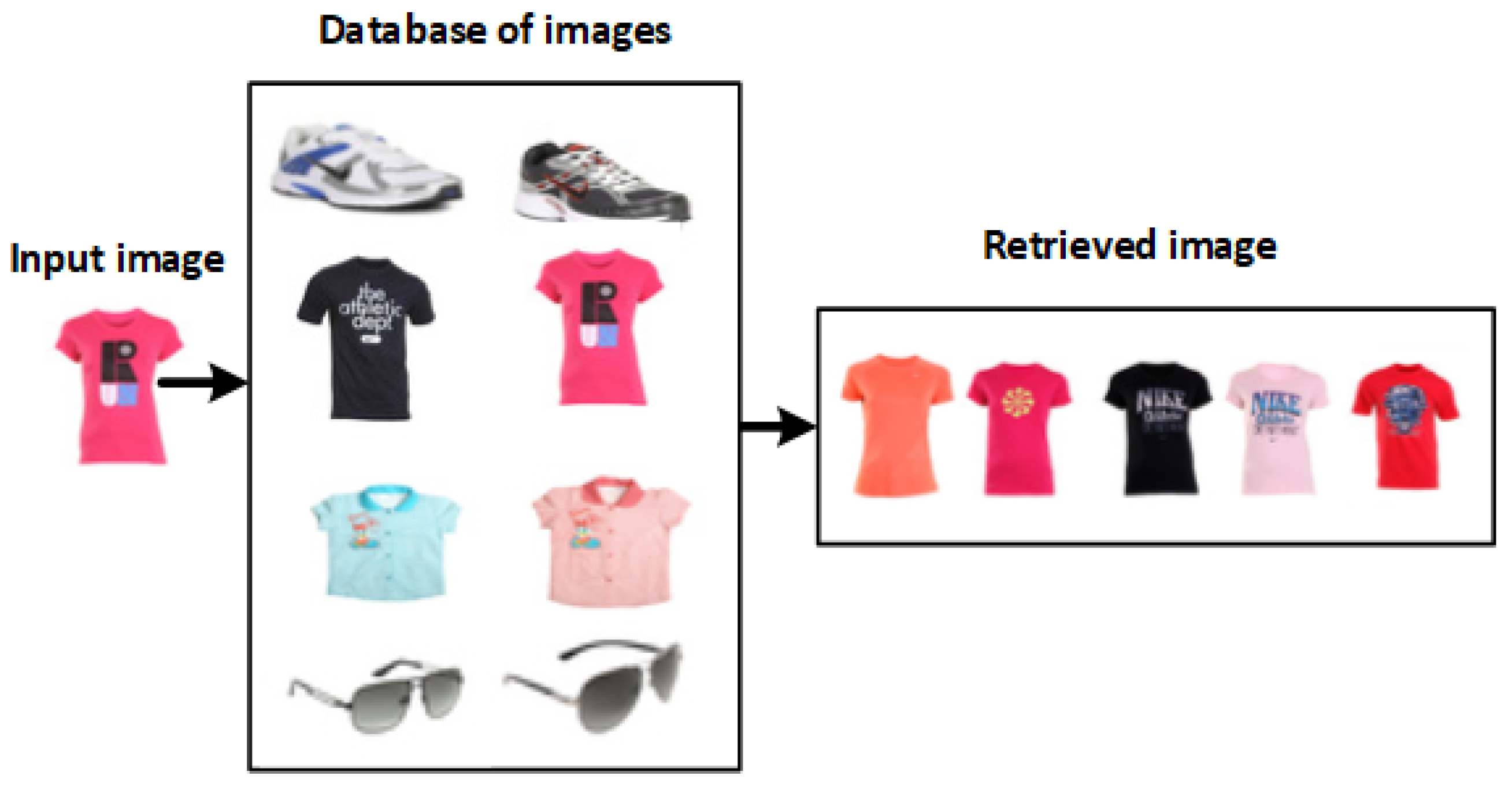
The Proposed Recommendation System Using DINOv2 Model and FAISS

This section outlines the methodology used to implement the recommendation system using the DINOv2 model for feature extraction and FAISS for an efficient nearest neighbor search. This methodology aims to demonstrate the effectiveness of DINOv2 features in retrieving nearest neighbor images from a given dataset.

Firstly, we employ the Gradio library [52] to create a user-friendly interface for interaction with the instance retrieval system. The interface allows users to upload images and immediately visualize the nearest neighbor images retrieved from the dataset. There are several main steps required to build a recommendation system, as shown in Figure 3.

• The interface allows users to upload an image, and then some of the transformation operations, such as resizing, tensor conversion, and normalization, are applied to the input image. Then, the extract_features function that is built into the DINOv2 model is applied to the transformed image to extract the features of the input image.
• We apply a nearest neighbor search with flat L2 index (Euclidean) distances to retrieve the similarity images from the database that is built in the FAISS library [53]. FAISS contains several similarity search methods. It assumes that the instances are represented as vectors and identified by an integer. The vectors can be compared with L2 (Euclidean) distances or dot products. Similar vectors are those with the lowest L2 distance or the highest dot product with the query vector. Our approach employs the FAISS library for an efficient nearest neighbor search. Central to this efficiency is the utilization of a flat L2 index. This data structure allows for the rapid retrieval of nearest neighbors based on Euclidean distances in the feature space. The following steps outline the process.
  • Index Creation: The feature vectors of the dataset images are indexed using the flat L2 index structure. This step preprocesses the dataset to facilitate quick distance calculations.
  • Distance Calculation: Given a query image’s feature vector, the flat L2 index computes the Euclidean distances between the query vector and all indexed vectors in the dataset.
  • Nearest Neighbor Identification: The index identifies the indices of dataset vectors with the smallest Euclidean distances to the query vector. These indices correspond to the nearest neighbor images.
  • Retrieval: The images associated with the nearest neighbor indices are retrieved from the dataset. These retrieved images are the nearest neighbors of the query image.

4. Experimental Results

4.1. Experimental Setup

In our study, we implemented the CNNs and pre-trained models using Keras, its Python API, running on a desktop PC with an Intel i7-6850K CPU and an NVIDIA GPU. The datasets were split into an 80% training set and a 20% testing set. We adapted some parameters for the CNN and pre-trained models: the number of epochs was 50, the activation function was softmax, the optimizer was Adam, and the loss function was categorical_crossentropy, with learning rate = 0.1. In the ViT model, some of the hyperparameters were adapted as shown in

Table 1. Hyperparameter configuration for ViT model.

Parameter	Value
input_size	28
learning_rate	0.001
weight_decay	0.0001
batch_size	256
num_epochs	50
image_size	72
num_patches	(72 // 6) × 2
projection_dim	64
num_heads	4
transformer_units	[64 × 2, 64]
transformer_layers	8
mlp_head_units	[2048, 1024]
normalization
resizing	72 × 72
random rotation	0.02
random zoom	0.02
loss function	categorical_crossentropy
activation function	softmax

.

Evaluating Models

Accuracy, precision, recall, the F1-score, the AUC, and ROC curves are metrics used to assess classification performance, as well as positive and negative predictions ($TP$ and $FP$). TN refers to the true negative state, $FN$ refers to the false negative state, $TP$ refers to the true positive state, and $FP$ refers to the false positive state, as demonstrated.

• Accuracy: During the classification of correctly classified instances, it shows the percentage of instances that are correctly classified.

  $$Accuracy=\frac{TP+TN}{TP+FP+TN+FN}.$$

  (1)
• Precision: The ratio between true positives and all positives.

  $$Precision=\frac{TP}{TP+FP}$$

  (2)
• The recall measures a model’s ability to correctly identify true positives.

  $$Recall=\frac{TP}{TP+FN}$$

  (3)
• F1-score: The precision and recall of the test values are used to calculate the F1-score.

  $$F1-score=\frac{2·precision·recall}{precision+recall}$$

  (4)
• Receiver operating characteristic curves (ROC) show how well classification models categorize data. It uses both the true positive and false positive parameters.
  In the case of true positives (TPR), commonly known as recall,

  $$\mathrm{True}\mathrm{positive}=\frac{\mathrm{True}\mathrm{positive}}{\mathrm{True}\mathrm{positive}+\mathrm{False}\mathrm{negative}}$$

  (5)
  FPR stands for the false positive rate, and it is defined as follows:

  $$\mathrm{False}\mathrm{positive}=\frac{\mathrm{False}\mathrm{positive}}{\mathrm{False}\mathrm{positive}+\mathrm{True}\mathrm{negative}}$$

  (6)
  On ROC curves, TPR and FPR are plotted against categorization levels. By lowering the categorization threshold, more items are classified as positive or false positive. As a result, both false positives and true positives increase.

4.2. The Results of Fashion-MNIST Dataset

This section compares the proposed stake model with other models. The results of models applied to Fashion-MNIST are shown in

Table 2. The results of Fashion-MNIST dataset.

Approach	Model	Accuracy	Precision	Recall	F1-Score
Pre-trained models	VGG16	89.29	89.21	89.29	89.19
	DenseNet-121	88.00	88.11	88.0	87.84
	Mobilenet	58.92	58.37	58.92	58.20
	ResNet50	84.53	84.69	84.53	84.38
Proposed CNN models	DeepCNN1	91.92	91.97	91.92	91.91
	Deep-CNN2	91.90	91.91	91.9	91.89
	Deep-CNN3	92.25	92.36	92.25	92.23
Transformer model	ViT	95.25	95.20	95.25	95.20

. As shown, the ViT model showed the highest performance (accuracy = 95.25, precision = 95.20, recall = 95.25, F1-score = 95.20), whereas Mobilenet showed the lowest performance (accuracy = 58.92, precision = 58.37, recall = 58.92, F1-score = 58.20).

We can see that the proposed CNN models recorded the highest performance compared to pre-trained models. Deep-CNN3 achieved the highest performance in terms of accuracy, precision, recall, and F1-score at 92.25, 92.36, 92.25, and 92.23, respectively, compared to DeepCNN1 and DeepCNN2. The ViT model improved the performance by 2% to 4% compared to the CNN models.

Figure 4 shows the ROC curve and AUC of DeepCNN3 for each class. Figure 5 shows each class’s ROC curve and AUC for the ViT model. The ROC curve is a graphical representation of a model’s performance across various threshold values for classification. It plots the true positive rate (TPR) against the false positive rate (FPR) as the threshold changes. The AUC is a single scalar value that quantifies the model’s overall performance. It represents the area under the ROC curve. We can see that the ROC curve for the ViT model shows the strong ability of the model to distinguish between positive and negative classes at different thresholds. ViT recorded the highest AUC for each class compared to DeepCNN3. For ViT, the AUC of eight classes was 1.00, and the AUC of two classes was 0.99, while the AUC of six classes was 100, the AUC of three classes was 0.99, and that of one class was 0.98.

4.3. The Results of Fashion Product Dataset

This section compares the proposed stake model with other models. The results of models applied to the fashion product dataset are shown in

Table 3. The results of fashion product dataset.

Approach	Model	Accuracy	Precision	Recall	F1-Score
Pre-trained model	VGG16	84.80	85.3	90.40	80.90
	DenseNet-121	77.66	77.918	78.75	77.11
	Mobilenet	75.55	75. 82	75.69	75.55
	ResNet50	82.23	82.53	82.23	82.53
Proposed CNN models	DeepCNN1	96.91	96.74	96.91	97.82
	Deep-CNN2	96.14	96.56	96.15	96.33
	Deep-CNN3	97.09	97.95	97.09	97.01
Transformer model	ViT	98.76	98.50	98.76	98.50

. As shown, ViT scored the highest results (accuracy = 98.76, precision = 98.50, recall = 98.76, F1-score = 98.50), whereas Mobilenet achieved the lowest results (accuracy = 75.55, precision = 75.82, recall = 75.69, F1-score = 75.55).

We can see that the proposed CNN models recorded the highest performance compared to pre-trained models. Deep-CNN3 achieved the highest performance (accuracy = 97.09, precision = 97.95, recall = 97.09, F1-score = 97.01) compared to DeepCNN1 and DeepCNN2. The ViT model improved the performance by 1% to 2% compared to CNN models.

Figure 6 shows the ROC curve and AUC of DeepCNN3 for each class. Figure 7 shows each class’s ROC curve and the AUC of the ViT model. The ROC curve is a graphical representation of a model’s performance across various threshold values for classification. It plots the true positive rate (TPR) against the false positive rate (FPR) as the threshold changes. The AUC is a single scalar value that quantifies the model’s overall performance. It represents the area under the ROC curve. We can see that the ROC curve for the ViT model shows the strong ability of the model to distinguish between positive and negative classes at different thresholds. ViT recorded the highest AUC for each class compared to DeepCNN3. For ViT, the AUC of five classes was 1.00, and the AUC of one class was 0.87.

4.4. The Best Models for Two Datasets

Figure 8 shows the best models for the Fashion-MNIST dataset. The highest results were recorded by ViT (accuracy = 95.25, precision = 95.20, recall = 95.25, F1-score = 95.20). The worst average rate was recorded by VGG16 (accuracy = 89.29, precision = 89.21, recall = 89.29, F1-score = 89.19).

Figure 9 shows the best models for the fashion product dataset. The highest results were recorded by ViT (accuracy = 98.76, precision = 98.50, recall = 98.76, F1-score = 98.50). The lowest were recorded by VGG16 (accuracy = 84.8, precision = 85.30, recall = 90.40, F1-score = 80.90).

4.5. Comparing the Proposed Model with Previous Studies

We compared the proposed model with other models, as shown in

Table 4. Comparing the proposed model with previous studies.

Paper	Dataset	Model	Performance
[17]	Fashion-MNIST	VGG16 H-CNN	Accuracy = 93
[18]	Fashion-MNIST	CNN	Accuracy = 93.5
[19]	Fashion-MNIST	SqueezeNet	Accuracy = 93.50
[20]	Fashion-MNIST	VGG-11	Accuracy = 91.5
[21]	Fashion-MNIST	CNN	Accuracy = 90
[55]	Fashion-MNIST	MCNN15	Accuracy = 94.04
[26]	Fashion Product Images	ResNet-50	Accuracy = 86.24
[54]	Fashion Product Images	DNN	Accuracy = 83.29
[56]	Fashion Product Images	VGG16	Accuracy = 83.96
Our work	Fashion-MNIST	ViT	Accuracy = 95.25
Our work	Fashion Product Images	ViT	Accuracy = 98.76

. The ViT models for the two datasets recorded the highest accuracy compared to other models. For Fashion-MNIST, the VGG16 H-CNN recorded 93% For fashion product images, ResNet-50 recorded 86.24% accuracy in [26]. In [54], the authors used a DNN with 83.29% accuracy.

Fashion Recommendation System Using DINOVA2

We test the fashion recommendation system using a private custom fashion image dataset collected from different resources and including different main categories, such as pullovers, shirts, trousers, watches, and shoes. We build an interface using the Gradio library [52] to allow users to upload images and visualize the retrieved similarity results, as shown in Figure 10. The coding of the fashion recommendation system has been uploaded to GitHub [57].

The main steps are as follows. (1) The user uploads images, and transformation operations such as resizing, tensor conversion, and normalization are applied to the input image; then, the extract_features function that is built into the DINOv2 model is applied to the transformed image to extract the features of the input image. (2) The similarity between the input image and the images from the database is calculated by the nearest neighbor search function that is built into the FAISS library with flat L2. It utilizes flat L2, a data structure that allows the rapid retrieval of nearest neighbors based on the Euclidean distances in the feature space. Using the flat L2 index significantly enhances the efficiency of the nearest neighbor search process, allowing for faster and more effective instance retrieval. Figure 11, Figure 12 and Figure 13 show examples of images that were uploaded, and the recommendation fashion system retrieved similar images.

5. Limitations

Despite the importance of our proposed model, it may bring several challenges related to the dataset and the implementation of the model, which could be summarized as follows.

• The performance of recommendation systems heavily relies on the availability and quality of data. One limitation is that our proposed system’s effectiveness is contingent upon the availability of comprehensive and accurate data related to user preferences, item characteristics, and user–item interactions. Limited or biased data can impact the system’s ability to generate accurate and diverse recommendations.
• The proposed system may face challenges in scenarios where there are limited or no historical data available for new users or items, which makes it difficult to personalize recommendations for users who have recently joined the platform or for new items that have a limited interaction history.
• As the user base and item catalog grow, the scalability of the recommendation system becomes crucial. The proposed system’s performance and efficiency might be affected when dealing with large-scale datasets and a high volume of concurrent user interactions.
• Our proposed system aims to provide accurate recommendations; ensuring diversity in the recommended items is also important. The system may have limitations in terms of generating diverse recommendations, which can impact user satisfaction and engagement.
• Although our research focused on the development and evaluation of the recommendation system, we did not conduct specific user feedback or evaluation experiments. Gathering direct user feedback and conducting user studies to assess user satisfaction, preferences, and system usability would provide valuable insights and further validate the effectiveness of the proposed system.

6. Conclusions

The study’s primary goal was to apply a Vision Transformer (ViT) to enhance the performance of the classification of fashion images using two public datasets. ViT is a set of transformer blocks consisting of a multi-head self-attention layer and a multilayer perceptron (MLP) layer. The hyperparameters of the ViT model were adapted to enhance the performance of the models. The ViT models were compared with CNN models and pre-trained models. CNN models consist of different layers, i.e., convolutional layers, multi-max pooling layers, multi-dropout layers, multi-fully connected layers, and a batch normalization layer. Accuracy, precision, recall, the F1-score, and the AUC were used to evaluate the models. The results showed that the proposed models achieved the highest performance values for two datasets. For the Fashion-MNIST dataset, ViT showed the highest performance (accuracy = 95.25, precision = 95.20, recall = 95.25, F1-score = 95.20) compared to other models. For the fashion product dataset, ViT LR showed the highest performance (accuracy = 98.53, precision = 98.42, recall = 98.53, F1-score = 98.46) compared to other models. A fashion recommendation system was developed using Learning Robust Visual Features without Supervision (DINOv2) and a nearest neighbor search built into the FAISS library to retrieve the top five similar images for specific images. The future work directions are as follows. (1) Conducting user studies and gathering direct user feedback are crucial steps to evaluate the proposed recommendation system. This can involve collecting user satisfaction ratings, conducting surveys or interviews to understand user preferences and perceptions, and comparing the system’s recommendations with user expectations. Incorporating user feedback will provide valuable insights for further refinement and improvement. (2) We could consider incorporating contextual information such as temporal dynamics, location, or social connections into the recommendation system. Context-aware recommendation algorithms can enhance the system’s ability to provide personalized and relevant recommendations by considering the situational context in which users interact with the system. (3) We could explore hybrid recommendation approaches that combine the strengths of different models or techniques. This could involve integrating content-based and collaborative filtering methods or combining deep learning models with traditional recommendation algorithms. (4) We could investigate methods to enhance the explainability and transparency of the recommendation system. Users often desire explanations as to why specific items are recommended to them. (5) We will consider evaluating the models using the Matthews correlation coefficient (MCC). (6) We intend to analyze the model from the complexity analysis perspective to ensure efficiency.

References

- Diaz, O.; Kushibar, K.; Osuala, R.; Linardos, A.; Garrucho, L.; Igual, L.; Radeva, P.; Prior, F.; Gkontra, P.; Lekadir, K. Data preparation for artificial intelligence in medical imaging: A comprehensive guide to open-access platforms and tools. Phys. Medica 2021, 83, 25–37. [Google Scholar] [CrossRef] [PubMed]
- Singh, A. Feature engineering for images: A valuable introduction to the HOG feature descriptor. Medium, Analytics Vidhya, 4 September 2019. [Google Scholar]
- Taye, M.M. Theoretical understanding of convolutional neural network: Concepts, architectures, applications, future directions. Computation 2023, 11, 52. [Google Scholar] [CrossRef]
- Elmannai, H.; Saleh, H.; Algarni, A.D.; Mashal, I.; Kwak, K.S.; El-Sappagh, S.; Mostafa, S. Diagnosis Myocardial Infarction Based on Stacking Ensemble of Convolutional Neural Network. Electronics 2022, 11, 3976. [Google Scholar] [CrossRef]
- Wu, J. Introduction to convolutional neural networks. arXiv 2017, arXiv:1511.08458. [Google Scholar]
- Kuang, Z.; Zhang, X.; Yu, J.; Li, Z.; Fan, J. Deep embedding of concept ontology for hierarchical fashion recognition. Neurocomputing 2021, 425, 191–206. [Google Scholar] [CrossRef]
- Goenka, S.; Zheng, Z.; Jaiswal, A.; Chada, R.; Wu, Y.; Hedau, V.; Natarajan, P. Fashionvlp: Vision language transformer for fashion retrieval with feedback. In Proceedings of the IEEE/CVF Conference on Computer Vision and Pattern Recognition, New Orleans, LA, USA, 18–24 June 2022; pp. 14105–14115. [Google Scholar]
- Chakraborty, S.; Hoque, M.S.; Rahman Jeem, N.; Biswas, M.C.; Bardhan, D.; Lobaton, E. Fashion recommendation systems, models and methods: A review. Informatics 2021, 8, 49. [Google Scholar] [CrossRef]
- Ma, Y.; Ding, Y.; Yang, X.; Liao, L.; Wong, W.K.; Chua, T.S. Knowledge enhanced neural fashion trend forecasting. In Proceedings of the 2020 International Conference on Multimedia Retrieval, Dublin, Ireland, 8–11 June 2020; pp. 82–90. [Google Scholar]
- Bazi, Y.; Bashmal, L.; Rahhal, M.M.A.; Dayil, R.A.; Ajlan, N.A. Vision transformers for remote sensing image classification. Remote Sens. 2021, 13, 516. [Google Scholar] [CrossRef]
- Chen, L.; Yang, F.; Yang, H. Image-Based Product Recommendation System with Convolutional Neural Networks; Stanford University: Stanford, CA, USA, 2017. [Google Scholar]
- Lin, Y.R.; Su, W.H.; Lin, C.H.; Wu, B.F.; Lin, C.H.; Yang, H.Y.; Chen, M.Y. Clothing recommendation system based on visual information analytics. In Proceedings of the 2019 International Automatic Control Conference (CACS), Keelung, Taiwan, 13–16 November 2019; pp. 1–6. [Google Scholar]
- Tuinhof, H.; Pirker, C.; Haltmeier, M. Image-based fashion product recommendation with deep learning. In Proceedings of the Machine Learning, Optimization, and Data Science: 4th International Conference, LOD 2018, Volterra, Italy, 13–16 September 2018; Revised Selected Papers 4. Springer: Berlin, Germany, 2019; pp. 472–481. [Google Scholar]
- Ko, H.; Lee, S.; Park, Y.; Choi, A. A survey of recommendation systems: Recommendation models, techniques, and application fields. Electronics 2022, 11, 141. [Google Scholar] [CrossRef]
- Sridevi, M.; ManikyaArun, N.; Sheshikala, M.; Sudarshan, E. Personalized fashion recommender system with image based neural networks. IOP Conf. Ser. Mater. Sci. Eng. 2020, 981, 022073. [Google Scholar] [CrossRef]
- Guan, C.; Qin, S.; Long, Y. Apparel-based deep learning system design for apparel style recommendation. Int. J. Cloth. Sci. Technol. 2019, 31, 376–389. [Google Scholar] [CrossRef]
- Seo, Y.; Shin, K.S. Hierarchical convolutional neural networks for fashion image classification. Expert Syst. Appl. 2019, 116, 328–339. [Google Scholar] [CrossRef]
- Kadam, S.S.; Adamuthe, A.C.; Patil, A.B. CNN model for image classification on MNIST and fashion-MNIST dataset. J. Sci. Res. 2020, 64, 374–384. [Google Scholar] [CrossRef]
- Meshkini, K.; Platos, J.; Ghassemain, H. An analysis of convolutional neural network for fashion images classification (fashion-mnist). In Proceedings of the Fourth International Scientific Conference “Intelligent Information Technologies for Industry” (IITI’19) 4, Prague, Czech Republic, 2–7 December 2019; pp. 85–95. [Google Scholar]
- Duan, C.; Yin, P.; Zhi, Y.; Li, X. Image classification of fashion-MNIST data set based on VGG network. In Proceedings of the 2019 2nd International Conference on Information Science and Electronic Technology (ISET 2019), Taiyuan, China, 21–22 September 2019; Volume 19. [Google Scholar]
- Vijayaraj, A.; Raj, V.; Jebakumar, R.; Gururama Senthilvel, P.; Kumar, N.; Suresh Kumar, R.; Dhanagopal, R. Deep learning image classification for fashion design. Wirel. Commun. Mob. Comput. 2022, 2022, 7549397. [Google Scholar] [CrossRef]
- Wazarkar, S.; Patil, S.; Gupta, P.S.; Singh, K.; Khandelwal, M.; Vaishnavi, C.S.; Kotecha, K. Advanced Fashion Recommendation System for Different Body Types using Deep Learning Models. Res. Sq. 2022. [Google Scholar] [CrossRef]
- Khalid, M.; Keming, M.; Hussain, T. Design and implementation of clothing fashion style recommendation system using deep learning. Rom. J. Inf. Technol. Autom. Control 2021, 31, 14. [Google Scholar] [CrossRef]
- Abdul Hussien, F.T.; Rahma, A.M.S.; Abdulwahab, H.B. An e-commerce recommendation system based on dynamic analysis of customer behavior. Sustainability 2021, 13, 10786. [Google Scholar] [CrossRef]
- Tayade, A.; Sejpal, V.; Khivasara, A. Deep Learning Based Product Recommendation System and its Applications. Int. Res. J. Eng. Technol. 2021, 8, 4. [Google Scholar]
- Liu, K.H.; Chuang, H.L.; Liu, T.J. Clothing recommendation based on deep learning. In Proceedings of the 2022 IEEE International Conference on Consumer Electronics, Osaka, Japan, 18–21 October 2022; pp. 281–282. [Google Scholar]
- Fashion MNIST. Available online: https://www.kaggle.com/datasets/zalando-research/fashionmnist (accessed on 5 July 2023).
- Fashion Product Images Dataset. Available online: https://www.kaggle.com/datasets/paramaggarwal/fashion-product-images-dataset (accessed on 9 July 2023).
- Vedaldi, A.; Zisserman, A. Vgg Convolutional Neural Networks Practical; Department of Engineering Science, University of Oxford: Oxford, UK, 2016; Volume 66. [Google Scholar]
- Bagaskara, A.; Suryanegara, M. Evaluation of VGG-16 and VGG-19 deep learning architecture for classifying dementia people. In Proceedings of the 2021 4th International Conference of Computer and Informatics Engineering (IC2IE), Depok, Indonesia, 14–15 September 2021; pp. 1–4. [Google Scholar]
- Belaid, O.N.; Loudini, M. Classification of brain tumor by combination of pre-trained vgg16 cnn. J. Inf. Technol. Manag. 2020, 12, 13–25. [Google Scholar]
- Zhou, Y.; Bai, Y.; Bhattacharyya, S.S.; Huttunen, H. Elastic neural networks for classification. In Proceedings of the 2019 IEEE International Conference on Artificial Intelligence Circuits and Systems (AICAS), Hsinchu, Taiwan, 18–20 March 2019; pp. 251–255. [Google Scholar]
- Albelwi, S.A. Deep Architecture based on DenseNet-121 Model for Weather Image Recognition. Int. J. Adv. Comput. Sci. Appl. 2022, 13, 10. [Google Scholar] [CrossRef]
- Hoeser, T.; Kuenzer, C. Object detection and image segmentation with deep learning on earth observation data: A review-part I: Evolution and recent trends. Remote Sens. 2020, 12, 1667. [Google Scholar] [CrossRef]
- Popescu, D.; Ichim, L.; Dimoiu, M.; Trufelea, R. Comparative Study of Neural Networks Used in Halyomorpha Halys Detection. In Proceedings of the 2022 30th Mediterranean Conference on Control and Automation (MED), Athens, Greece, 28 June–1 July 2022; pp. 182–187. [Google Scholar]
- Theckedath, D.; Sedamkar, R. Detecting affect states using VGG16, ResNet50 and SE-ResNet50 networks. SN Comput. Sci. 2020, 1, 1–7. [Google Scholar] [CrossRef]
- Chu, Y.; Yue, X.; Yu, L.; Sergei, M.; Wang, Z. Automatic image captioning based on ResNet50 and LSTM with soft attention. Wirel. Commun. Mob. Comput. 2020, 2020, 8909458. [Google Scholar] [CrossRef]
- Elpeltagy, M.; Sallam, H. Automatic prediction of COVID-19 from chest images using modified ResNet50. Multimed. Tools Appl. 2021, 80, 26451–26463. [Google Scholar] [CrossRef] [PubMed]
- Albawi, S.; Mohammed, T.A.; Al-Zawi, S. Understanding of a convolutional neural network. In Proceedings of the 2017 International Conference on Engineering and Technology (ICET), Antalya, Turkey, 21–23 August 2017; pp. 1–6. [Google Scholar]
- Brownlee, J. A Gentle Introduction to Pooling Layers for Convolutional Neural Networks. 2019. Available online: https://machinelearningmastery.com/pooling-layers-for-convolutional-neural-networks/ (accessed on 22 August 2023).
- Basha, S.S.; Dubey, S.R.; Pulabaigari, V.; Mukherjee, S. Impact of fully connected layers on performance of convolutional neural networks for image classification. Neurocomputing 2020, 378, 112–119. [Google Scholar] [CrossRef]
- Bisong, E.; Bisong, E. Regularization for deep learning. In Building Machine Learning and Deep Learning Models on Google Cloud Platform: A Comprehensive Guide for Beginners; Apress: Berkeley, CA, USA, 2019; pp. 415–421. [Google Scholar]
- Tolstikhin, I.O.; Houlsby, N.; Kolesnikov, A.; Beyer, L.; Zhai, X.; Unterthiner, T.; Yung, J.; Steiner, A.; Keysers, D.; Uszkoreit, J.; et al. Mlp-mixer: An all-mlp architecture for vision. Adv. Neural Inf. Process. Syst. 2021, 34, 24261–24272. [Google Scholar]
- Agarwal, P.; Vempati, S.; Borar, S. Personalizing similar product recommendations in fashion e-commerce. arXiv 2018, arXiv:1806.11371. [Google Scholar]
- Wong, W.K.; Zeng, X.; Au, W.; Mok, P.Y.; Leung, S.Y.S. A fashion mix-and-match expert system for fashion retailers using fuzzy screening approach. Expert Syst. Appl. 2009, 36, 1750–1764. [Google Scholar] [CrossRef]
- Lahitani, A.R.; Permanasari, A.E.; Setiawan, N.A. Cosine similarity to determine similarity measure: Study case in online essay assessment. In Proceedings of the 2016 4th International Conference on Cyber and IT Service Management, Bandung, Indonesia, 26–27 April 2016; pp. 1–6. [Google Scholar]
- Cleophas, T.J.; Zwinderman, A.H. Modern Bayesian Statistics in Clinical Research; Technical Report; Springer: Berlin, Germany, 2018. [Google Scholar]
- Good, P. Robustness of Pearson correlation. Interstat 2009, 15, 1–6. [Google Scholar]
- Zou, K.H.; Tuncali, K.; Silverman, S.G. Correlation and simple linear regression. Radiology 2003, 227, 617–628. [Google Scholar] [CrossRef]
- Vittayakorn, S.; Yamaguchi, K.; Berg, A.C.; Berg, T.L. Runway to realway: Visual analysis of fashion. In Proceedings of the 2015 IEEE Winter Conference on Applications of Computer Vision, Lake Tahoe, NV, USA, 12–15 March 2015; pp. 951–958. [Google Scholar]
- Arslan, T. A weighted Euclidean distance based TOPSIS method for modeling public subjective judgments. Asia-Pac. J. Oper. Res. 2017, 34, 1750004. [Google Scholar] [CrossRef]
- Gradio App. Available online: https://www.gradio.app (accessed on 22 August 2023).
- Johnson, J.; Douze, M.; Jégou, H. Billion-scale similarity search with GPUs. IEEE Trans. Big Data 2019, 7, 535–547. [Google Scholar] [CrossRef]
- Gharaei, N.Y.; Dadkhah, C.; Daryoush, L. Content-based clothing recommender system using deep neural network. In Proceedings of the 2021 26th International Computer Conference, Computer Society of Iran (CSICC), Tehran, Iran, 3–4 March 2021; pp. 1–6. [Google Scholar]
- Nocentini, O.; Kim, J.; Bashir, M.Z.; Cavallo, F. Image classification using multiple convolutional neural networks on the fashion-MNIST dataset. Sensors 2022, 22, 9544. [Google Scholar] [CrossRef]
- Rohrmanstorfer, S.; Komarov, M.; Mödritscher, F. Image classification for the automatic feature extraction in human worn fashion data. Mathematics 2021, 9, 624. [Google Scholar] [CrossRef]
- Coding of Recommendation System. Available online: https://github.com/hagersalehahmed/recommendation_system (accessed on 22 August 2023).