1. Introduction
Across geosciences, many investigated phenomena relate to specific complex systems consisting of intricately intertwined interacting subsystems. These can be suitably represented as networks, an approach that is gaining increasing attention in the complex systems community [
1,
2]. The meaning of the existence of a link between nodes of a network depends on the area of application, but in many cases it is related to some form of information exchange between the nodes.
This approach has already been adopted for the analysis of various phenomena in the global climate system [
3,
4,
5,
6,
7]. For a recent review discussing the progress, opportunities and challenges, see [
8]. Typically, a graph is constructed by considering two locations linked by a connection, if there is an instantaneous dependence between the localized values of a variable of interest.
This dependence can be conveniently quantified by mutual information, an entropy-based general measure of statistical dependence that takes into account nonlinear contributions to the coupling. In practice, for reasons of theoretical and numerical simplicity, linear Pearson’s correlation coefficient might be sufficient, although potentially neglecting the nonlinear contributions to interactions. In particular, while initial works by Donges
et al. stressed the role of mutual information in detecting important features of global climate networks [
9,
10], more detailed recent work has shown that the differences between correlation and mutual information graphs are mostly (but not necessarily completely) spurious, such as due to natural and instrumental (related to data collection) nonstationarities of the data [
11].
However, these methods do not allow to assess the directionality of the links and of the underlying information flow. This motivates the use of more sophisticated measures, known also as causality analysis methods. Indeed, it has been recently suggested that data-driven detection of climate causality networks could be used for deriving hypotheses about causal relationships between prominent modes of atmospheric variability [
12,
13].
The family of causality methods include linear approaches such as Granger causality analysis [
14], as well as more general nonlinear methods. A prominent representative of nonlinear causality assessment is the conditional mutual information [
15], especially in the form of transfer entropy [
16].
Arguably, the nonlinear methods, due to their model-free nature, have the theoretical advantage of being sensitive to forms of interactions that linear methods may detect only partially or not at all. On the other hand, this advantage may be more than outweighed by a potentially lower precision. Depending on specific circumstances, this may adversely affect the reliability of the detection of network patterns.
Apart from uncertainty about the general network pattern, reliability is important when the focus lies on detecting changes in time, with the need to distinguish them from random variability of the estimates among different sections of time series under investigation—a task that is relevant in many areas of geoscience including climate research. In other words, before analyzing a complex dynamical system using network theory, a key initial question is that of the reliability of the network construction, and how it depends on the choice of a causality method and its parameters.
We study this question for a selection of standard causality methods, using a timely application in the study of a climate network and its variability. In particular, surface air temperature data from the NCEP/NCAR reanalysis dataset [
17,
18] is used. The original data contains more than 10,000 time series—a relatively dense grid covering the whole globe. For efficient computation and visualization of the results, it is convenient to reduce the dimensionality of the data. We use principal component analysis and select only components that have significantly high explained variance compared with the corresponding spatially independent but temporally dependent (
i.e., “colored”) random noise.
As the causality network construction reliability may crucially depend on the specific choice of causality estimator, we test different causality measures and their parametrization by quantifying the similarity of causality matrices reconstructed from independent realizations of a stationary model of data. These realizations are either independently generated, or they represent individual non-overlapping temporal windows of a single stationary realization. Optimal parameter choices of the applied nonlinear methods are detected, and the reliability of networks constructed using linear and nonlinear methods is compared. The latter method, i.e., comparing networks reconstructed from temporal windows, allows also to assess the network variability on real data and to compare it with the variability observed in the analysis of stationary model time series.
2. Data and Methods
2.1. Causality Assessment Methods
2.1.1. Granger Causality Analysis
A prominent method for assessing causality is Granger causality analysis, named after Sir Clive Granger, who proposed this approach to time series analysis in a classical paper [
14]. However, the basic idea can be traced back to Wiener [
19], who proposed that if the prediction of one time series can be improved by incorporating the knowledge of a second time series, then the latter can be said to have a causal influence on the former. This idea was formalized by Granger in the context of linear regression models. In the following, we outline the methods of assessment of Granger causality, following the description given in [
20,
21,
22].
Consider two stochastic processes
and
and assume they are jointly stationary. Let further the autoregressive representations of each process be:
and joint autoregressive representation
where the covariance matrix of the noise terms is:
The causal influence from
Y to
X is then quantified based on the decrease in the residual model variance when we include the past of
Y in the model of
X,
i.e., when we move from the independent model given by Equation (
1) to the joint model given by Equation (
3):
Similarly, the causal influence from
X to
Y is defined as:
Clearly, the causal influence defined in this way is always nonnegative.
The original introduction of the concept of statistical inference of causality [
14] includes a third (potentially highly multivariate) process
Z, representing all other intervening processes that should be controlled for in assessing the causality between
X and
Y. The bivariate (or “pairwise”) implementation of the estimator thus constitutes a computational simplification of the original process, for the sake of numerical stability as well as comparability with the bivariate transfer entropy (conditional mutual information) approach introduced later. See
Section 4 for further discussion of related issues.
2.2. Estimation of GC
Practical estimation of Granger causality involves fitting the joint and univariate models described above to experimental data. While the theoretical framework is formulated in terms of infinite sums, the fitting procedure requires selection of the model order p for the models. For our report, we have selected , corresponding to links of lag 1, since this lag was also chosen in the nonlinear methods considered later. This is a common choice for Granger causality in literature and amounts to looking for links with lag 1 time unit.
2.3. Transfer Entropy
The information-theoretic analog to Granger causality is the concept of
transfer entropy (TE [
16]). TE can be defined in terms of
conditional mutual information as shown below, closely following [
15]. In particular, we can define that
X causes
Y if the knowledge of the past of
X decreases the uncertainty about
Y (above what the knowledge of past of
Y and potentially all other relevant confounding variables already informs).
For two discrete random variables
with sets of values Ξ and
Υ and probability distribution functions (PDFs)
and joint PDF
, the Shannon entropy
is defined as
and the joint entropy
of
X and
Y as
The conditional entropy
of
X given
Y is
The amount of shared information contained in the variables
X and
Y is quantified by the mutual information
defined as
The conditional mutual information
of the variables
given the variable
Z is given as
Entropy and mutual information are measured in bits if the base of the logarithms in their definitions is 2. It is straightforward to extend these definitions to more variables, and to continuous rather than discrete variables.
The transfer entropy from
X to
Y then corresponds to the conditional mutual information between
and
conditional on
:
While the definition of these information-theoretic functionals is very general and elegant, the practical estimation faces challenges related to the problem of efficient estimation of the PDF from finite size samples. It is important to bear in mind the distinction between the quantities of the underlying stochastic process and their finite-sample estimators.
2.4. Potential Causes of Observed Difference
Interestingly, it can be shown that for linear Gaussian processes, transfer entropy is equivalent to linear Granger causality, up to a multiplicative factor [
23]:
However, in practice, the estimates of transfer entropy and linear Granger causality may differ. There are principally two main reasons for this divergence between the results. Firstly, when the underlying process is not linear Gaussian, the true transfer entropy may differ from the true linear Granger causality corresponding to the linear approximation of the process. A second reason for divergence between sample estimates of transfer entropy and linear Granger causality, valid even for linear Gaussian processes, is the difference in the properties of the estimators of these two quantities, in particular bias and variance of the estimates.
2.5. TE Estimation
There are many algorithms for the estimation of information-theoretical functionals that can be adapted to compute transfer entropy estimates. Two basic classes of nonparametric methods for the estimation of conditional mutual information are the
binning methods and the
metric methods. The former discretize the space into regions usually called bins or boxes—a robust example is the equiquantal method based on discretization of studied variables into
Q equiquantal bins (EQQ [
24]). In the latter methods, the probability distribution function estimation depends on the distances between the samples computed using some metric. An example of a metric method is the
k-nearest neighbor (kNN [
15,
25]) algorithm. For more detail on methods of estimation of conditional mutual information and their comparison, see [
15].
Note that both types of algorithms require setting an additional parameter. While some heuristic suggestions have been published in the literature, suitable values of these parameters may depend on specific aspects of the application including the character of the time series. For the purpose of this study, we use a range of parameter values and subsequently select the parameter values providing the most stable results for further comparison with linear methods, see below.
2.6. Data
2.6.1. Dataset
Data from the NCEP/NCAR reanalysis dataset [
17] has been used. In particular, we utilize the time series
of daily and monthly mean surface air temperature from January 1948 to December 2007 (
and
time points, respectively), sampled at latitudes
and longitude
forming a regular grid with a step of
. The points located at the poles have been removed, giving a total of
spatial sampling points.
2.6.2. Preprocessing
To minimize the bias introduced by periodic changes due to solar irradiation, the mean annual cycle has been removed to produce anomaly time series. The data were further standardized such that the time series at each grid point has unit variance. The time series are then scaled by the cosine of the latitude to account for grid points closer to the poles representing smaller areas and being closer together (thus biasing the correlation with respect to grid points farther apart). The poles are thus omitted entirely by effectively removing data for latitude .
2.6.3. Computing the Components
First, the covariance matrix of the scaled time series obtained by preprocessing is computed. Note that this covariance matrix is equal to the correlation matrix, where each correlation is scaled by the inverse of the product of the cosines of the latitudes of the time series entering the correlation.
Next, the eigendecomposition of the covariance matrix is computed. The eigenvectors corresponding to genuine components are extracted (the estimation of the number of components is explained in the next paragraph). The eigenvectors are then rotated using the VARIMAX method [
26].
The rotated eigenvectors are the resulting components. Each component is represented by a scalar field of intensities over the globe, and by a corresponding time series. See
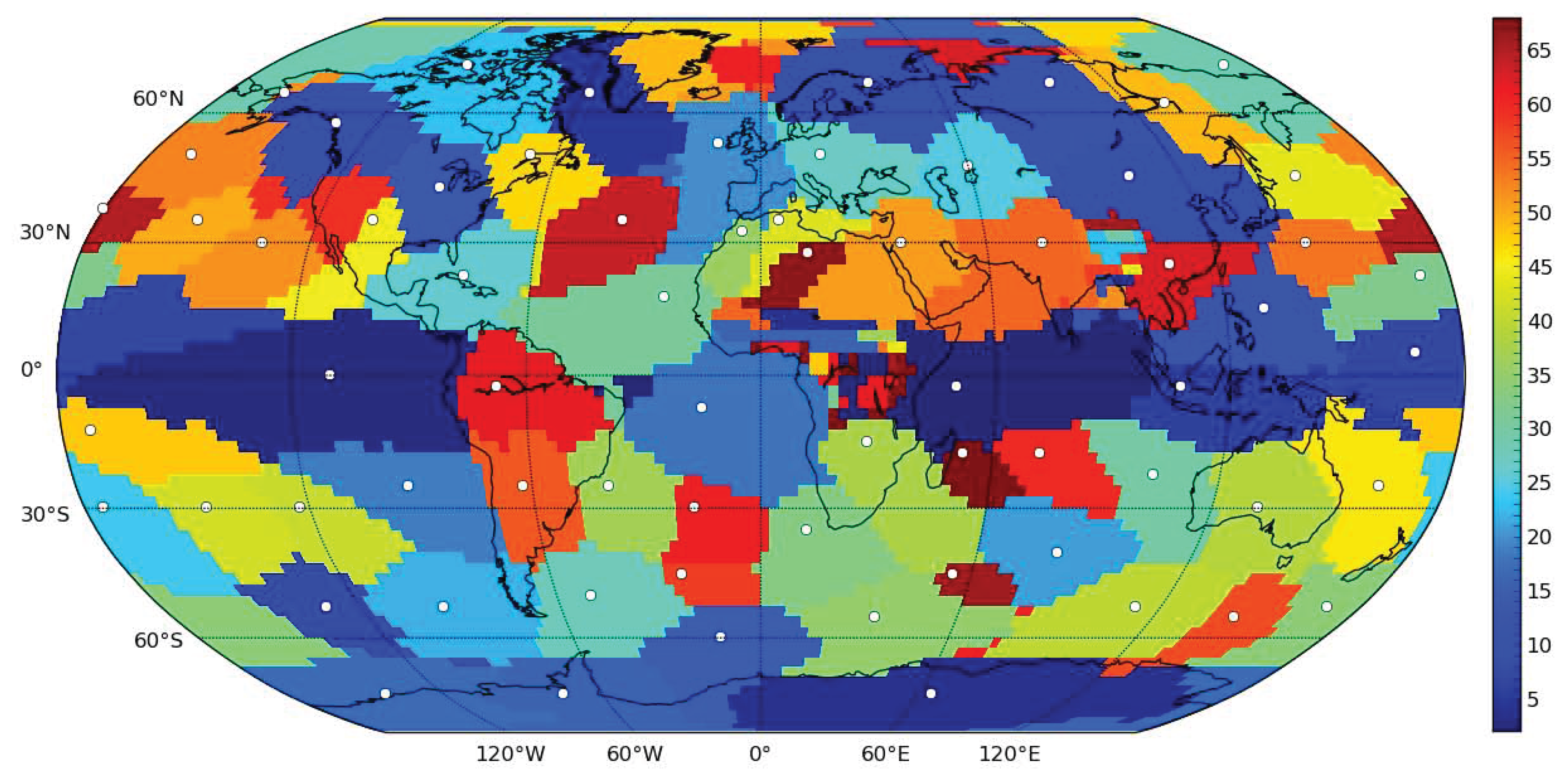
Figure 1 for a parcellation of the globe by the components. For each location, the color corresponding to the component with maximal intensity is used—due to good spatial localization and smoothness of the components, this leads to the parcellation of the globe into generally contiguous regions.
Figure 1.
Location of areas dominated by specific components of the surface air temperature data using VARIMAX-rotated PCA decomposition. For each location, the color corresponding to the component with maximal intensity was used. White dots represent approximate centers of mass of the components, used in subsequent figures for visualization of the nodes of the networks.
2.6.4. Estimating the Dimensionality of the Data
To reduce the dimensionality, only a subset of the components is selected for further analysis. The main idea rests in determining significant components by comparing the eigenvalues computed from the original data to eigenvalues computed from a control dataset corresponding to the null hypothesis of uncoupled time series with the same temporal structure as the original data. To accomplish this, the time series in the control datasets are generated as realizations of autoregressive (AR) models that are fitted to each time series independently. The dimension of the AR process is estimated for each time series separately using the Bayesian Information Criterion [
27].
This model is used to generate 10,000 realizations in the control dataset. The eigendecomposition of each realization is computed and aggregated, providing a distribution for each eigenvalue (1st, 2nd, ...) under the above null hypothesis. Finding the significant eigenvalues then reduces to a multiple comparison problem, which we resolved using the False Discovery Rate (FDR) technique [
28], leading to the identification of 67 components.
For computational reasons, the decomposition was carried out on the monthly data and the resulting component weights were used to extract daily time series from the corresponding preprocessed daily data (anomalization, standardization, cosine transform). The method thus provides full-resolution component localization on the 10224-point grid while also yielding a high-resolution time series associated with each component. Indeed, carrying out the decomposition directly on the daily data might have provided a slightly different set of components, as the decomposition would also take into account high-frequency variability. The current decomposition has both conceptual and practical motivation. Conceptually, it provides information about the high-frequency behavior of the variability modes detected in the monthly data (a timescale more commonly used for decomposition in the climate community). The practical reason is that the decomposition of the full matrix of daily data is computationally demanding, particularly in combination with the bootstrap testing procedure described above.
2.7. Network Construction
Formally, in the graph-theoretical approach, a network is represented by a graph , where V is the set of nodes of G, is the number of nodes and is the set of the edges (or links) of G. In weighted graphs, each edge connecting nodes i and j can be assigned a weight representing the strength of the link. Thus, the pairwise causality matrix with entries can be understood as a weighted graph. Commonly, the graph is transformed into an unweighted matrix by suitable thresholding, keeping only links with weights higher than some threshold (and setting their weights to 1) while removing the weaker links (setting their weights to zero).
There are three principal strategies to choose the threshold. One can choose a fixed value based on expert judgment of what constitutes a strong link, or adaptively to enforce a required density of the graph (relative number of links with respect to the maximum number possible, i.e., in a full graph of given size). The third option is to use statistical testing to detect statistically significant links. In the current paper, we start with the original unthresholded graphs, but provide also example results for thresholded graphs using the above approaches.
2.8. Reliability Assessment
In line with the terminology of psychometrics or classical test theory, by reliability we mean the overall consistency of a measure (consistency here does not mean the statistical sense of asymptotic behavior). In the context of network construction, we considered a method reliable if the networks constructed from different samples of the same dynamical process are similar to each other. Note that this does not necessarily imply validity or accuracy of the method—under some circumstances, a method could consistently arrive at wrong results. In a way, reliability/consistency can be considered a first step to validity. In practical terms, even if the validity was undoubted, reliability can give the researcher an estimate on the confidence he/she can have in the reproducibility of the results.
To assess the similarity of two matrices, many methods are available, including the (entry-wise) Pearson’s linear correlation coefficient. Inspection of the causality matrices suggests a heavily non-normal distribution of the values with many outliers. Therefore, the correlation of ranks, using Spearman’s correlation coefficient, may be more suitable.
Apart from reliability of the full weighted causality graphs, we also study the unweighted graphs derived by thresholding. Based on inspection of the causality matrices, a density of 0.01 (keeping 1 percent of strongest links) was chosen for the analysis. To assess the similarity of two binary matrices, we use the Jaccard similarity coefficient. This is the relative number of links that are shared by the matrices with respect to the total number of links that appear at least in one of the matrices. Such a ratio is a natural measure of matrix overlap, ranging from 0 for matrices with no common links to 1 for identical matrices.
2.8.1. Model
A convenient method for assessing the reliability of a method on time series is to compare the results obtained from different temporal windows. However, dissimilarity among the results can be theoretically attributed to both lack of reliability of the method and hypothetical true changes in the underlying system over time (nonstationarity).
Therefore, to isolate the effect of method properties, we test the methods on a realistic but stationary model of the data. To provide such a stationary model of the potentially non-stationary data, surrogate time series were constructed.
Technically, surrogate time series are conveniently constructed as multivariate Fourier transform (FT) surrogates [
29,
30]. They are computed by first performing a Fourier transform of the series and keeping unchanged the magnitudes of the Fourier coefficients (the amplitude spectrum). Then the same random number is added to the phases of coefficients of the same frequency bin. The surrogate is then the inverse FT into the time domain.
The surrogate data represent a realization of a linear stationary process conserving the linear structure (covariance and autocovariance) of the original data, and hence also the linear component of causality. Note that any nonlinear component of causality should be removed, and the nonlinear methods should therefore converge to the linear methods (as discussed in
Section 2.1).
After testing the reliability on the stationary linear model, we assess the stability of the methods also on real data. The variability here should reflect a mixture of method non-reliability and true climate changes. Note that also the nonlinear methods may potentially diverge from the linear ones due to nonlinear causalities in the data.
2.8.2. Implementation Details
For estimation, both the stationary model and the real data time series were split into 6 windows (one for each decade, i.e., with approximately 3650 time points). For each of the windows, the causality matrix has been estimated with several causality methods.
In particular, we have used pairwise Granger causality as a representative linear method and computed transfer entropy by two standard algorithms using a range of critical parameter values. The first is an algorithm based on the discretization of studied variables into
Q equiquantal bins (EQQ [
24],
) and the second is a
k-nearest neighbor algorithm (kNN[
15,
25],
).
Each of these algorithms provides a matrix of causality estimates among the 67 climate components within the respective decade. We further assess the similarity of these matrices across both time and methods, first in stationary data (where temporal variability is attributable to method instability only) and then in real data. Apart from direct visualization, the similarity of the constructed causality matrices is quantified by the Spearman’s rank correlation coefficient of off-diagonal entries. The reliability is then estimated as the average Spearman’s rank correlation coefficient across all pairs of temporal windows.
To inspect the robustness of the results, the analysis was repeated with several possible alterations to the approach. Firstly, the similarity among the thresholded rather than unweighted graphs was assessed by means of the Jaccard similarity coefficient instead of Spearman’s rank correlation coefficient. Secondly, we repeated the analysis using linear multivariate AR(1) process for the generation of the stationary model instead of Fourier surrogates. Thirdly, the analysis was repeated on sub-sampled data (by averaging each 6 days to give one data point). This way, the same methods should provide causality on a longer time scale. To keep the same (and sufficiently high) number of time points, the sub-sampled data were not split into windows, but 6 realizations were generated from a fitted multivariate AR(1) process.
Finally, to assess the role that the reliability of different methods may have for statistical inference, we tested the number of links that the method was able to statistically distinguish compared with an empirical distribution corresponding to independent linear processes. This null hypothesis was realized by computing the causalities on a set of univariate Fourier surrogates. Under the hypothesis of no dependence between the processes, the probability of the data’s causality value for a given pair of variables being the highest among the total 20 values available is , providing a convenient nonparametric test of causality.
4. Discussion
The series of examinations provided evidence that both nonlinear and linear methods may be used to construct directed climate networks in a reliable way under a range of settings, with the basic linear Granger causality outperforming the studied nonlinear methods. On the side of nonlinear causality methods, we focused on the prominent family of methods based on the estimation of conditional mutual information in the form of transfer entropy. Two algorithms were used that represent key approaches of estimating conditional mutual information and have been extensively used and proven efficient on real-world data. Alternative approaches also exist, including the use of recurrence plots [
31].
Indeed, for the sake of tractability, we have limited the investigation in several ways. As the motivation of the current study was to explore the rationale for use of linear/nonlinear methods in causal climate network construction and to provide a basis for more detailed analyses of climate networks, some simple pragmatic methodological choices have been made mainly for testing the method’s differences, rather than studying specific phenomena.
Most prominently, linear Granger causality was chosen for its theoretical equivalence to transfer entropy (under the assumption of linearity), as this provides a fair comparison. However, the use of the strictly pairwise causality estimators suffers from severe inherent limitations. To give an example, a system consisting of three processes
, where
Z drives both
X and
Y, but with different temporal lags, may erroneously show causal influence between
X and
Y even though these were not directly coupled. To deal with such situations, the concepts can be generalized to the multivariate case [
32]. In the case of linear Granger causality this leads to fitting a multivariate linear process including, apart form
X and
Y, also a (possibly multivariate)
Z.
On the other side, there is a price for including too many variables in the model, as for short time series the theoretical advantage of including possible common causes may be outweighed by the numerical instability of fitting a higher order model. In
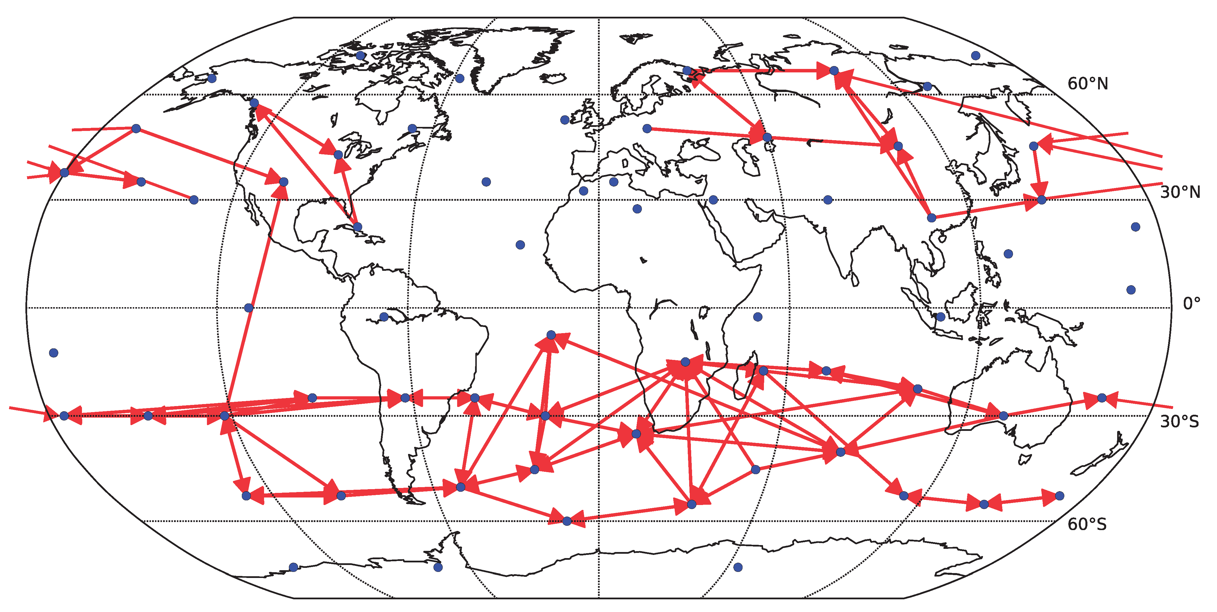
Figure 9 we include an example result for applying the fully multivariate linear Granger causality, with the pairwise causality for each pair taking into account variability explained by all the other 65 component time series. Note that many of the links recovered by the simplified bivariate linear Granger causality are recovered (see
Figure 7), however, the multivariate model leads to the detection of many long-ranging links crossing the equator, which are likely spurious and a result of lower reliability of the algorithm. Quantitatively, the average similarity (Spearman’s rank correlation coefficient) among the multivariate linear Granger causality matrices obtained for six decades of linear surrogate data was
, compared with
obtained for the simplified bivariate linear Granger causality. We do not provide analogous results for nonlinear methods, as the estimation of information-theoretical functionals in the fully multivariate setting is computationally prohibitively difficult.
Figure 9.
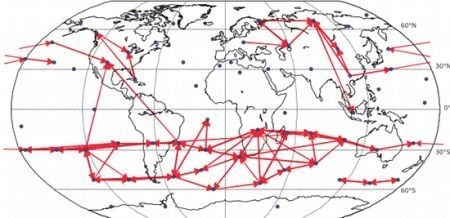
Causality network obtained by averaging the results for the six decades (total time span 1948–2007) for decomposed data (67 components represented by center of mass). Only the 100 strongest links are shown. For each decade, the network was detected by the fully multivariate linear Granger causality.
Figure 9.
Causality network obtained by averaging the results for the six decades (total time span 1948–2007) for decomposed data (67 components represented by center of mass). Only the 100 strongest links are shown. For each decade, the network was detected by the fully multivariate linear Granger causality.
Similarly, the assumption of a single possible lag (1 time step of 1 or 6 days respectively in our investigation) may not be suitable in real context, although at least the relative reliability of different methods may not be strongly affected by this within reasonable range of parameters. For precise geophysical interpretation, fitting an appropriate model order and allowing multiple lags would be warranted.
In general, estimation of these generalized causality patterns from relatively short time series is technically challenging, particularly in the context of nonlinear, information-theory based causality measures, due to the exponentially increasing dimension of probability distributions to be estimated. However, recent work has provided promising approaches to tackle this curse of dimensionality by decomposing TE into low-dimensional contributions [
32]. For theoretical and numerical considerations on how a causal coupling strength can be defined in the multivariate context, see [
33]. Assessment of the performance of these novel methods in the detection of causal climate networks is a subject of future work. For completeness we mention that apart from the time-domain treatment of causality, the whole problem can also be reformulated in the spectral domain, leading to frequency-resolved causality indices such as partial directed coherence (PDC [
34]) or Directed Transfer Function (DTC [
35]).
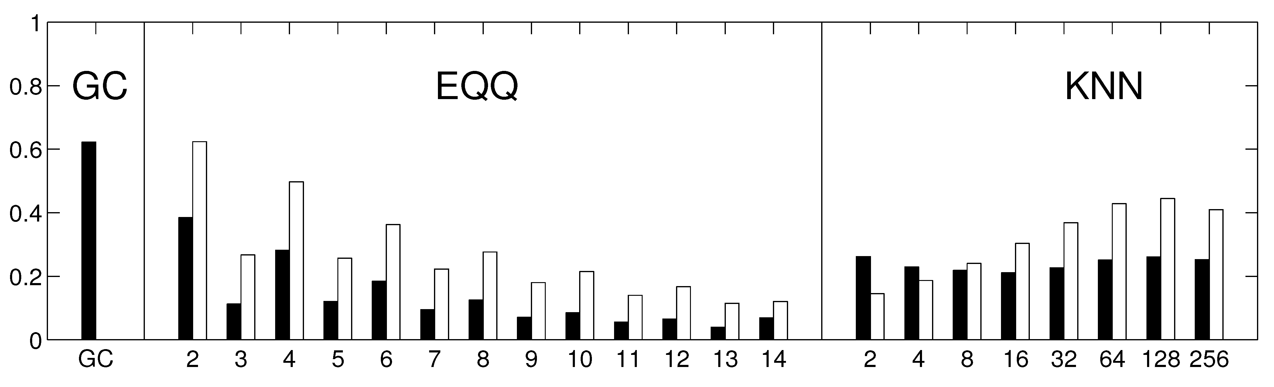
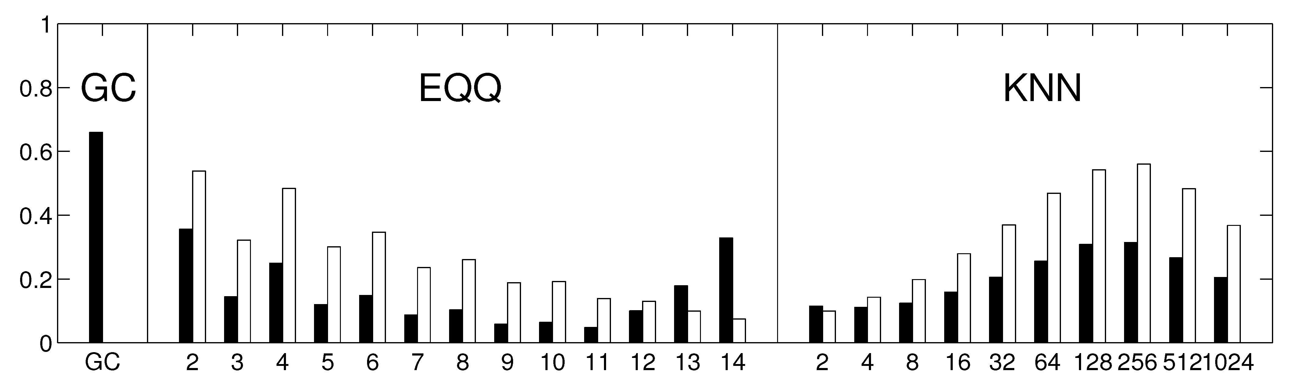
Our study also shows some key properties of the conditional mutual information estimates. Note that for instance for the 6-days networks (
Figure 5), the EQQ method reliability increases again for
, however, the similarity to the linear estimate further decreases. A direct check of the causality networks shows that they tend to a trivial column-wise structure, with the intensities for each column highly correlated to the autoregressive coefficient of the given time series. This corresponds to a manifestation of a dominant autocorrelation-dependent bias in the EQQ estimator for too high
Q values (note that
corresponds to less than one time point per average in a 4D bin, an unsuitable sampling of the space for effective probability distribution function approximation).
Reconstruction of networks directly from gridded climatic field data is challenging and perhaps not always the best approach, for reasons including efficient computation and visualization of the results. Instead, we apply here a decomposition of the data in order to get the most important components, i.e., by using a varimax-rotated principle component analysis. This provides a useful dimension-reduction of the studied problem. In particular, the gridded data does not reflect the real climate subsystems, which may be better approximated by the decomposition modes. However, as the decomposition is an implicit (weighted) coarse-graining, the detected difference between the linear and nonlinear methods may be different from that in the original time series data. In particular, the spatial averaging may increase the reliability of both approaches by suppressing noise, but also suppress any highly spatially localized heterogeneous patterns of both nonlinear and linear character. This might be reflected in the specific results of the paper, in particular the obtained quantitative reliability estimates.
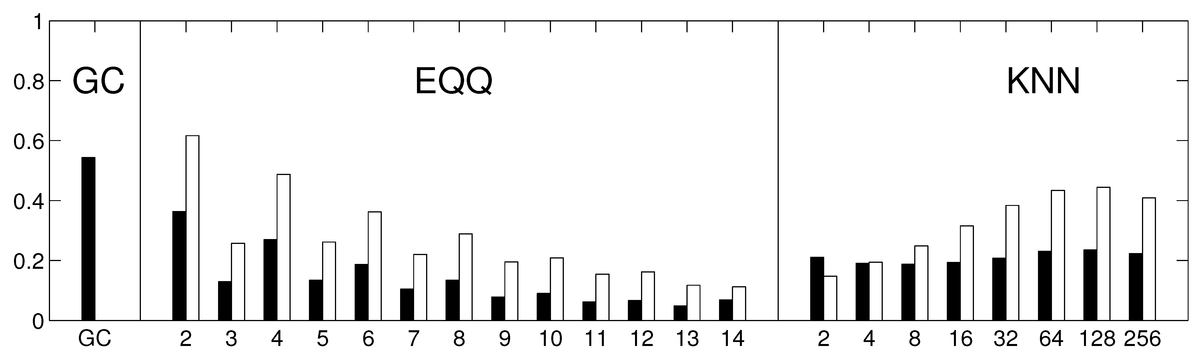
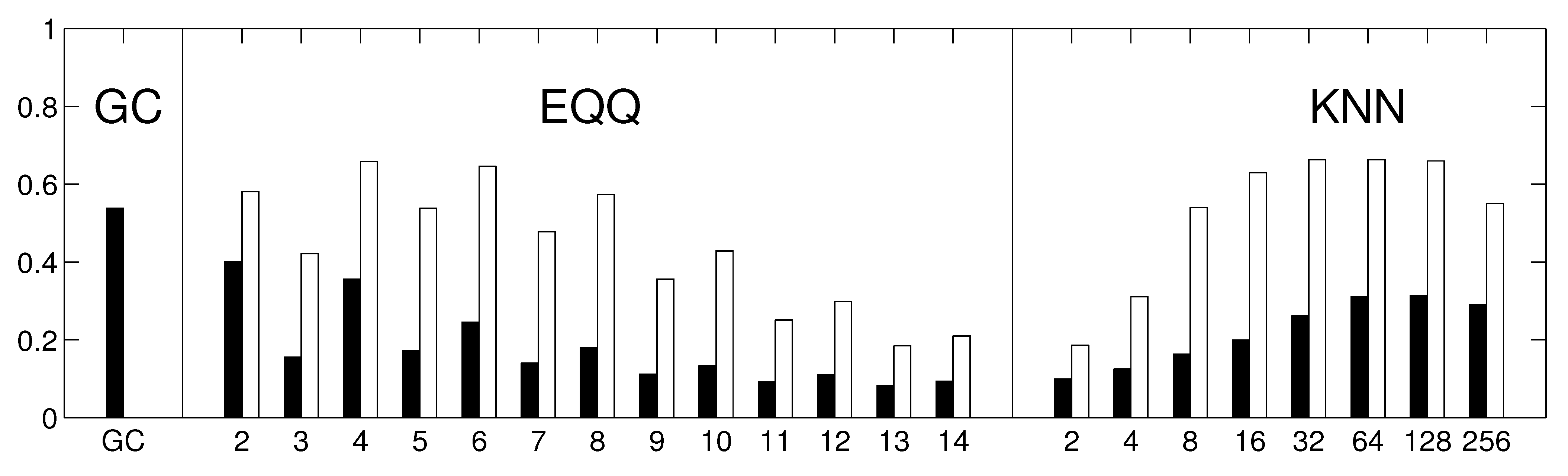
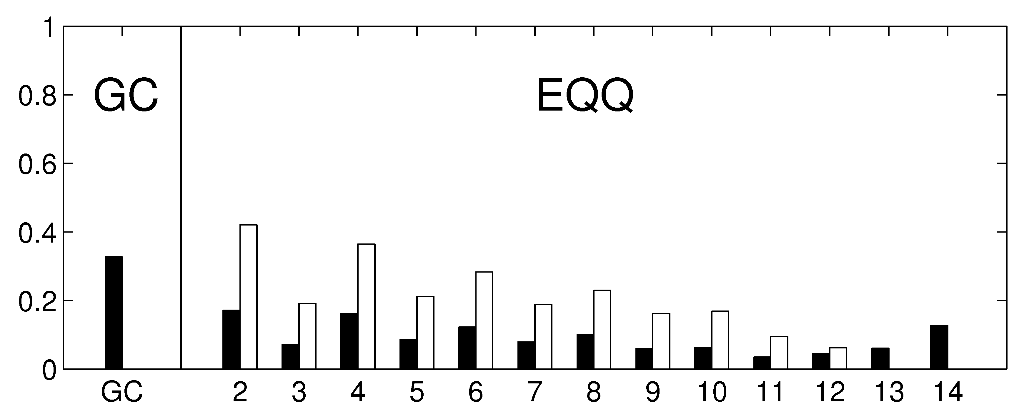
To assess how the results generalize to gridded data, we carried out a partial analysis using an approximately equidistant grid consisting of 162 spatial locations. The time series were preprocessed by removing anomalies in mean as well as in variance. The reliability assessment for the gridded data shows qualitatively similar results, see
Figure 10. As for the component data, the linear Granger causality has proven to be most reliable, and also relatively reliable results are obtained for nonlinear conditional mutual information with a small number of bins (
). The overall decrease in reliability is probably due to a combination or larger matrix size and less sophisticated dimensionality reduction strategy. The kNN algorithm was not assessed on this data to limit additional computational time demands. The average graphs for linear and nonlinear causality are shown in
Figure 11 and
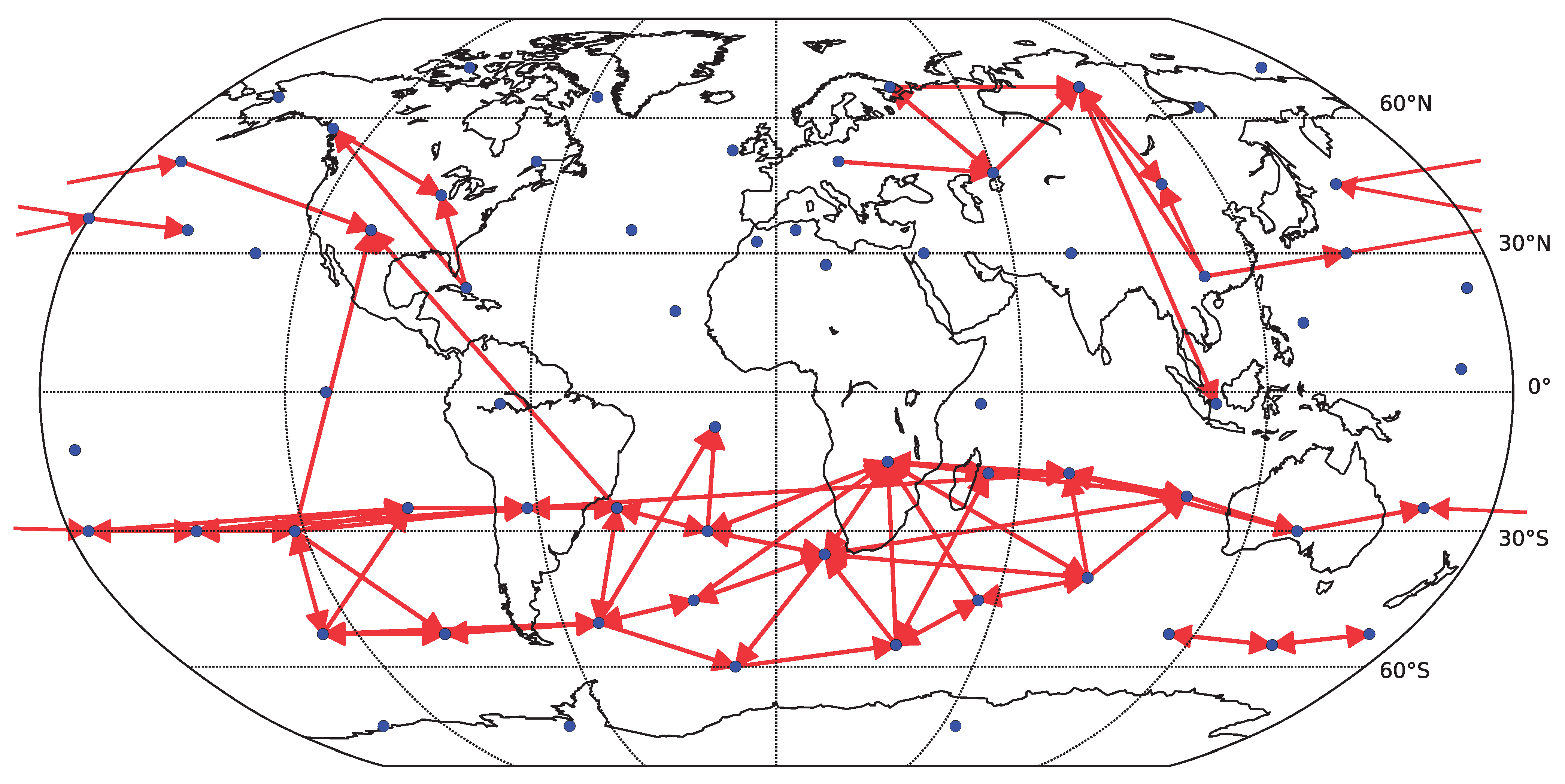
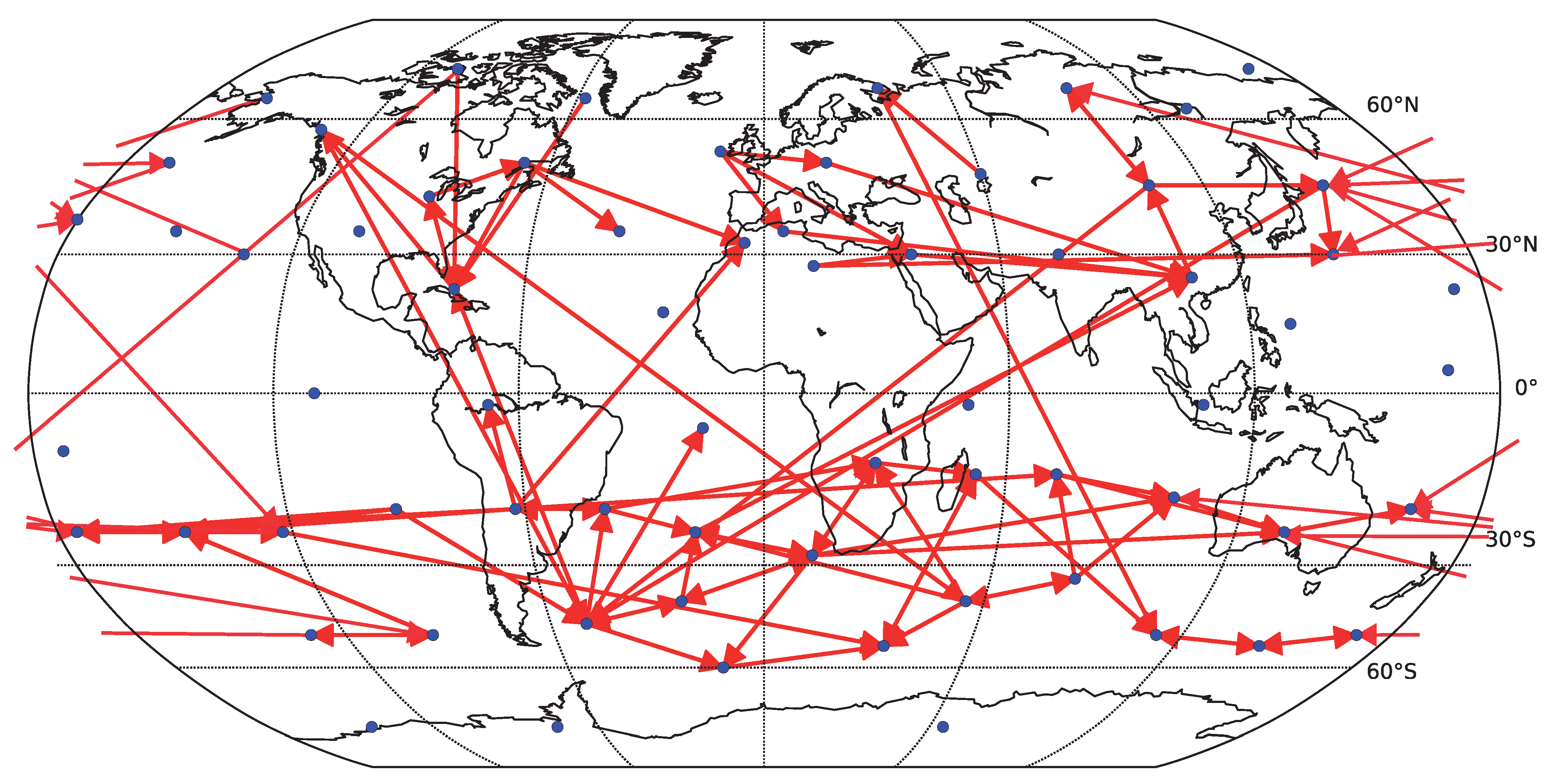
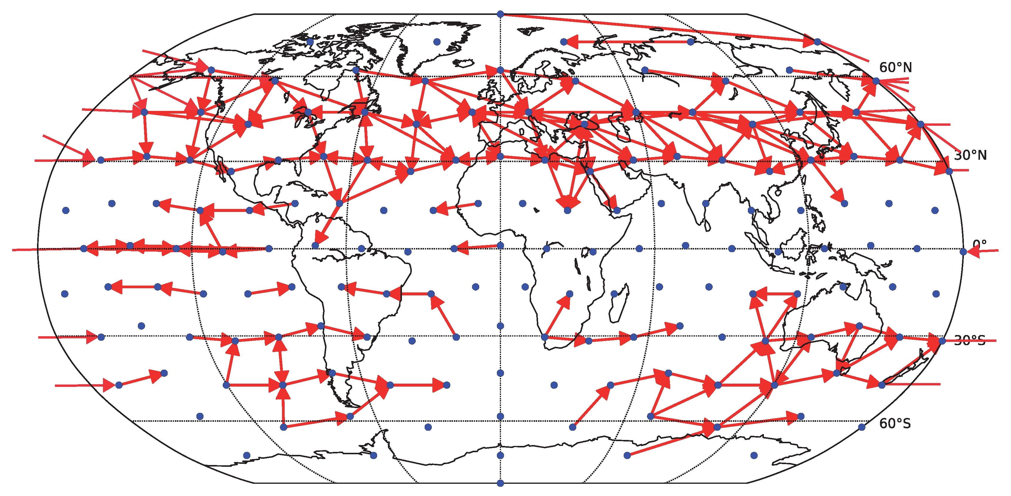
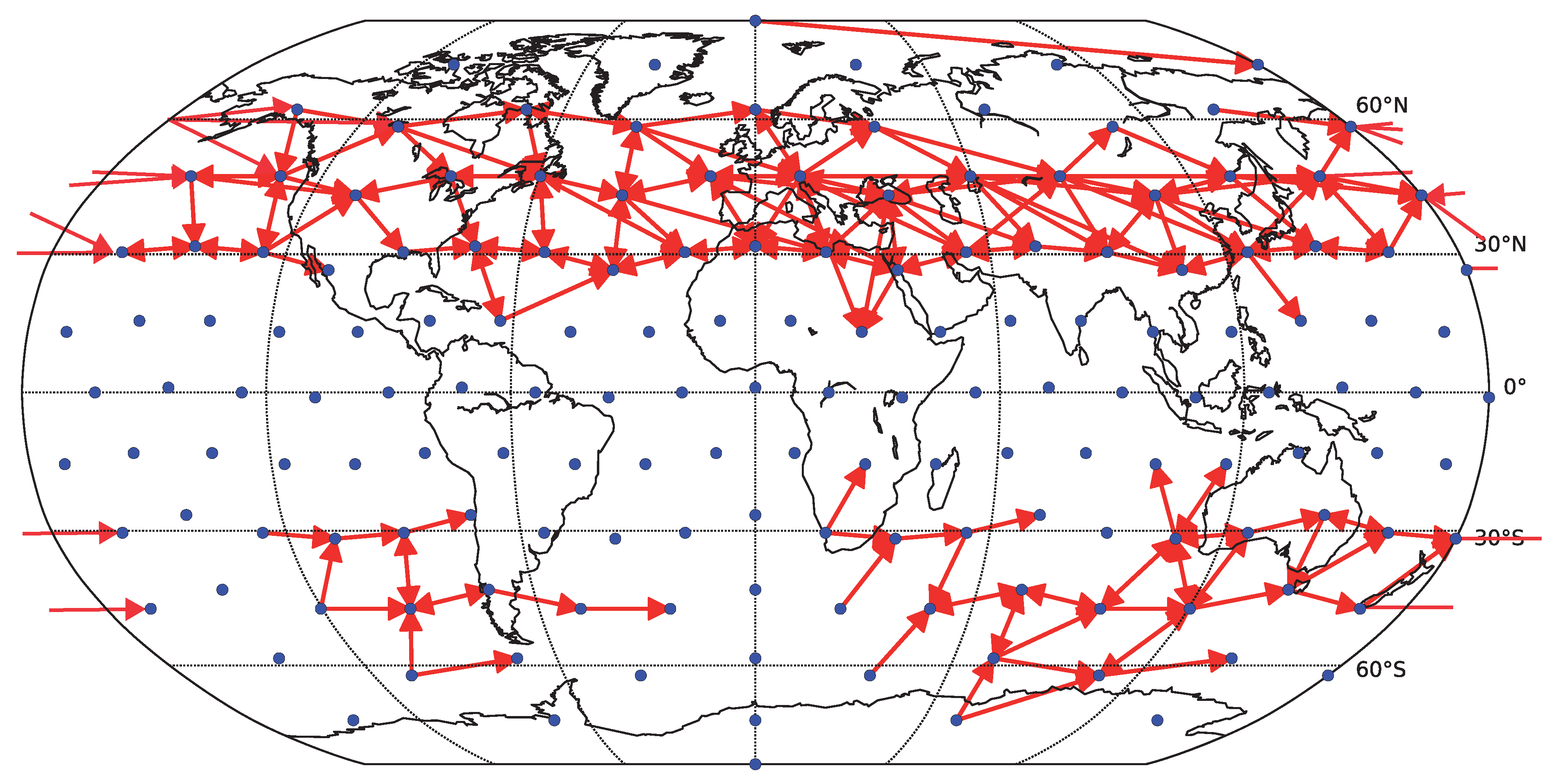
Figure 12 respectively. Interestingly, the spatial sparsity may be more suited to the 1-day lag causality estimation, as the detected average causality graphs hold structure that is easier to interpret. In particular, the direction of detected information flow in the extra-tropical areas approximately between
and
on both hemispheres almost without exception resembles the prevailing eastward direction of air circulation in the Ferrell cells (mid-latitude westerlies). On the other side, in particular the graph in
Figure 11, the direction of detected information flow corresponding to the strongest 200 links for the more robust linear Granger causality method also includes many arrows aiming westwards in the tropical regions (e.g., in the Pacific), which may correspond to the easterly trade winds in the regions corresponding to Hadley cells.
Figure 10.
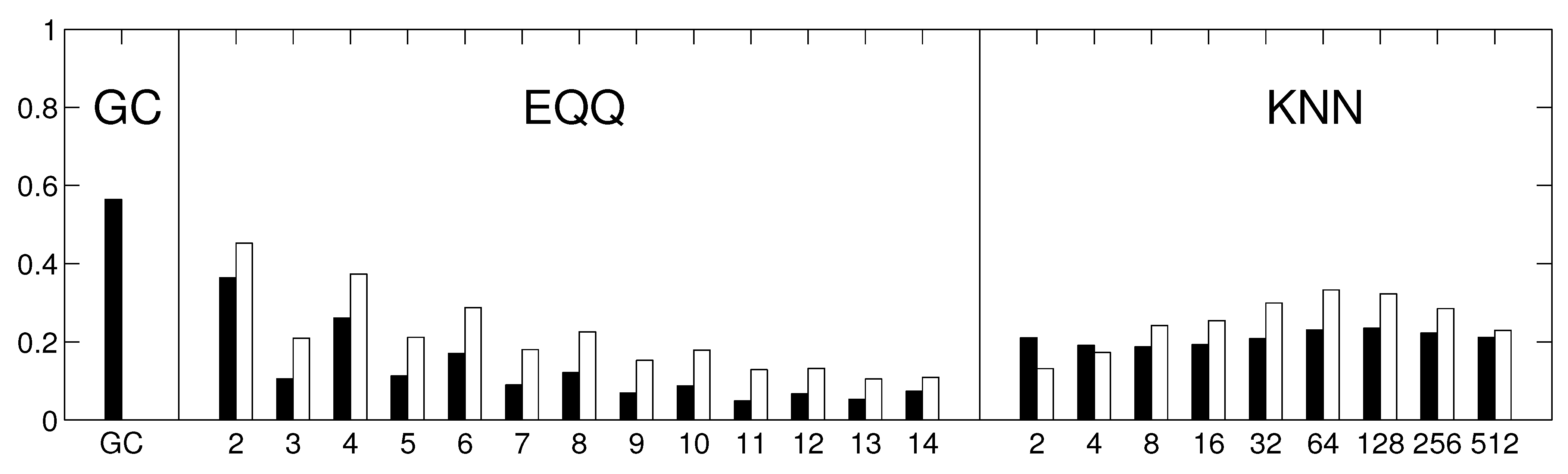
The reliability of causality network detection using different causality estimators and the similarity to linear causality network estimates for the Fourier surrogates model. For each estimator, six causality networks are estimated, one for each decade-long section of the model stationary data (a Fourier surrogate realization of the original data). Black: the height of the bar corresponds to the average Spearman’s correlation across all 15 pairs of decades. White: the height of the bar corresponds to the average Spearman’s correlation of nonlinear causality network and linear causality network across 6 decades.
Figure 10.
The reliability of causality network detection using different causality estimators and the similarity to linear causality network estimates for the Fourier surrogates model. For each estimator, six causality networks are estimated, one for each decade-long section of the model stationary data (a Fourier surrogate realization of the original data). Black: the height of the bar corresponds to the average Spearman’s correlation across all 15 pairs of decades. White: the height of the bar corresponds to the average Spearman’s correlation of nonlinear causality network and linear causality network across 6 decades.
Figure 11.
Causality network obtained by averaging the results for the six decades (total time span 1948–2007) for gridded data (162 spatial locations). Only the 200 strongest links are shown. For each decade, the network was estimated by linear Granger causality.
Figure 11.
Causality network obtained by averaging the results for the six decades (total time span 1948–2007) for gridded data (162 spatial locations). Only the 200 strongest links are shown. For each decade, the network was estimated by linear Granger causality.
Figure 12.
Causality network obtained by averaging the results for the six decades (total time span 1948–2007) for gridded data (162 spatial locations). Only the 200 strongest links are shown. For each decade, the network was estimated by (nonlinear) conditional mutual information, using the equiqantal binning method with .
In general, the differences in reliability may have important consequences for the detectability of causal links as well as their changes. Of course, theoretically this is not necessary since a nonlinear system may have links that have negligible linear causality but strong enough nonlinear causality fingerprint. Recent works have proposed approaches for the explicit quantification of the nonlinear contribution of equal-time dependence [
36], applied to neuroscientific [
36] as well as climate data [
11]. However, the generalization to higher dimensional information-theoretic functionals is not straightforward and is the subject of ongoing work. Thus, we give here at least an illustrative example of the trade-off between the generality of transfer entropy and the higher reliability of linear Granger causality: using the original 67 components data (divided into 6 decadal sections, see
Section 2), the basic statistical test at the 5% significant level (described in
Section 2) marked on average 1592 links as statistically significant (out of 4422 possible), while the EQQ method showed in general a lower number of significant links, depending on the parameter value in a way similar to the reliability estimate, with a maximum of 983 significant links for
and a minimum of 287 significant links for
. Note that given the significance level of the test, on average
significant links would be expected to appear by chance in a collection of completely unrelated processes.
5. Conclusions
A meaningful interpretation of climate networks and their observed temporal variability requires knowledge and minimization of the methodological limitations. In the present work, we discussed the problem of the reliability of network construction from time series of finite length, quantitatively assessing the reliability for a selection of standard bivariate causality methods. These included two major algorithms for estimating transfer entropy with a wide range of parameter choices, as well as linear Granger causality analysis, which can be understood as linear approximation of transfer entropy. Overall, the causality methods provided reproducible estimates of climate causality networks, with the linear approximations outperforming the studied nonlinear methods in reliability. Interestingly, optimizing the nonlinear methods with respect to reliability has led to improved similarity of the detected networks to those discovered by linear methods, in line with the hypothesis of near-linearity of the investigated climate reanalysis data, in particular the surface air temperature time series.
The latter hypothesis regarding the surface air temperature has been supported by the study in [
11] which extended the older results of [
37] who tested for possible nonlinearity in the dynamics of the station (Prague-Klementinum) SAT time series and found that the dependence between the SAT time series
and its lagged twin
was well-explained by a linear stochastic process. This result about a linear character of the temporal evolution of SAT time series, as well as the results of the present study, cannot be understood as arguments for a linear character of atmospheric dynamics
per se. Rather, these results characterize the properties of measurement or reanalysis data at a particularly coarse level of resolution. The data, thus, reflect a spatially and temporally averaged mixture of dynamical processes. For instance, a closer look on the dynamics of the specific temporal scales in temperature and other meteorological data has led to the identification of oscillatory phenomena with nonlinear behavior, exhibiting phase synchronization [
38,
39,
40,
41,
42]. Also the leading modes of atmospheric variability exhibit nonlinear behavior [
43,
44] and can Inferring the directionality of coupling with conditional mutual information. in a nonlinear way [
45].
Further work is needed to assess the usability and advantages of more sophisticated, recently proposed causality estimation methods. The current work also provides an important step towards the reliable characterization of climate networks and the detection of potential changes over time.

 ,
, 


