Multi-Granulation Entropy and Its Applications

Abstract

In the view of granular computing, some general uncertainty measures are proposed through single-granulation by generalizing Shannon’s entropy. However, in the practical environment we need to describe concurrently a target concept through multiple binary relations. In this paper, we extend the classical information entropy model to a multi-granulation entropy model (MGE) by using a series of general binary relations. Two types of MGE are discussed. Moreover, a number of theorems are obtained. It can be concluded that the single-granulation entropy is the special instance of MGE. We employ the proposed model to evaluate the significance of the attributes for classification. A forward greedy search algorithm for feature selection is constructed. The experimental results show that the proposed method presents an effective solution for feature analysis.

1. Introduction

Uncertainty analysis represents one of the most significant challenging tasks in intelligent computation. Since Shannon introduced the information entropy to measure the uncertainty of the system, a series of measures were proposed for machine learning, data mining and pattern recognition, etc. [1,2,3].

In the field of granular computing, Yu et al. introduced the fuzzy entropy for attribute reduction [4]. Hu et al. presented kernel entropy by extended Yu’s work [5]. In [6], the authors defined neighborhood entropy by using a neighborhood relation. In the view of granular computing, there are two modules in the entropy methodology mentioned above: (1) granulation of data (samples) into a set of information granules according to the relation of objects; (2) calculating the sum of the uncertainty quantity of all the information granules. We will give an example to illustrate this two-step process in detail in Section 2. It shows that granulation plays a key role in these entropy models. However, the classical information entropy theory utilizes solely the granularity structure of the given data, which is expressed by one suitable binary relation. The neighborhood entropy is only based on the neighborhood granulation; the fuzzy entropy on the fuzzy granulation; and the kernel entropy on the kernel granulation. In [7], Qian at el. proposed that there is a contradiction between two different binary relations in some data analysis issues. In other words, the decision or the view of each of decision makers may be independent for the same object in the process of some decision making. Accordingly, Qian et al. proposed multi-granulation rough set (MGRS) according to a user’s different requirements or targets of problem solving. Since then, many researchers have extended the classical MGRS by using various generalized binary relations. Lin et al. [8] proposed a covering-based pessimistic multi-granulation rough set. Xu et al. [9] proposed another generalized version, called variable precision multi-granulation rough set. There are two essential problems to be addressed when employing the rough sets model to real-world applications as similar as the information entropy model: (1) information granulation [10,11]; (2) approximate classification realized in the presence of such induced information granules [12,13]. The idea of multi-granulation is expressed through the approximation classification realizing. For example, one of the contributions in MGRS is to describe the lower and upper approximations by the multiple equivalence relations instead of the single equivalence relation. As a matter of fact, we can construct the multi-granulation structure in the process of the information granulation. Based on this idea, the contribution of this paper includes: (1) we extend the classical information entropy model to a multi-granulation entropy model (MGE) by using a series of general binary relations; (2) moreover, a number of theorems are obtained; (3) furthermore, we employ the proposed model to evaluate the significance of the attributes for classification. A forward greedy search algorithm for feature selection is constructed. The experimental results show that the proposed method presents an effective solution for feature analysis.

The paper is organized as follows: in Section 2, some basic concepts about entropy in the view of granular computing are briefly reviewed. In Section 3, the MGE model is proposed. A series of theorems about MGE is discussed. Section 4 shows the applications of MGE to feature evaluating and feature selection. Numeric experiments are reported in Section 5. Finally, Section 6 concludes the paper.

2. Entropy in the View of Granular Computing

Knowledge representation is realized via the information system ($IS$) which is a tabular form, similar to databases. An information system is pair $IS=\left(U,A\right)$, where $U=\left\{x_1,x_2,\dots ,x_n\right\}$ is a nonempty finite set of objects, $A$ is a nonempty finite set of attributes, and $f_a:U\to V_a$ is a mapping for any $a\in A$, where $V_a$ is called the value set of $a$.

Relations, as a fundamental concept in mathematics, represent the connections of a set elements in the domain. A binary relation on $U$ can be represented as a matrix. The matrix $M_R={\left(r_{ij}\right)}_{n\times n}$ is called the relation matrix of $R$ on the universe $U$. The matrix $M_R={\left(r_{ij}\right)}_{n\times n}$ is denoted as:

$$M_R=\left(\begin{array}{cccc}{r}_{11}& r_{12}& \cdots & r_{1n}\\ r_{21}& r_{22}& \cdots & r_{2n}\\ ⋮& ⋮& ⋮& ⋮\\ r_{n1}& r_{n2}& \cdots & r_{nn}\end{array}\right)$$

(1)

In the classical set theory, the relations take values in the set $\left\{0,1\right\}$. In this case the relation matrix is a Boolean matrix. In the fuzzy set theory, the relations take values in the interval $\left[0,1\right]$. In this paper, we use a general binary relation $R$ to denote any instantiated relation, such as fuzzy relation and kernel relation, etc. The fuzziness of relations is the essential characteristic in these cases. Therefore, $r_{ij}\in \left[0,1\right]$ in our study.

Given an information system $IS=\left(U,A\right)$ and a binary relation $R$, $U=\left\{x_1,x_2,\dots ,x_n\right\}$, $\forall x_i\in U$ the information granule ${\left[x_i\right]}_R$ is defined as:

$${\left[x_i\right]}_R=\frac{r_{1i}}{x_1}+\frac{r_{2i}}{x_2}+\cdots +\frac{r_{ni}}{x_n}$$

(2)

With each sample, we express the information granule in the form of fuzzy sets. Here, we give an instance about kernel entropy to illustrate the information entropy model in the view of kernel granulation [5]:

Example 1. Given an information system $IS=\left(U,A\right)$ as follows:

Table 1. $IS$ description.

	$a_1$	$a_2$
$x_1$	0.1	0.4
$x_2$	0.2	0.3

Table 1. $IS$ description.

	$a_1$	$a_2$
$x_1$	0.1	0.4
$x_2$	0.2	0.3

where $U=\left\{x_1,x_2\right\}$ and $A=\left\{a_1,a_2\right\}$, the two modules in the kernel entropy methodology are as follows, respectively:

(1) Information granulation:

The kernel relation is computed with Gaussian kernel as follows, where $\Vert x_i-x_j\Vert$ is the Euclidean distance between samples $x_i$ and $x_j$:

$$r_{ij}=\exp \left(-\frac{{\Vert x_i-x_j\Vert }^2}{2{\sigma }^2}\right)$$

(3)

Hence, we have $r_{12}=r_{21}\approx 0.37$ and $r_{11}=r_{22}=1$ if $\sigma$ is set to 0.1. The kernel granules can be constructed according Equation (2).

(2) Calculating the kernel entropy:

The cardinality of ${\left[x_i\right]}_R$ is computed in the form of $\left|{\left[x_i\right]}_R\right|={\displaystyle {\sum }_{j=1}^n{r}_{ij}}$. Thus, the expected cardinality of ${\left[x_i\right]}_R$ is computed as follows, where $\left|U\right|$ is cardinality of set $U$.

$$\overline{Card}\left({\left[x_i\right]}_R\right)=\frac{\left|{\left[x_i\right]}_R\right|}{\left|U\right|}$$

(4)

The kernel entropy is defined as follows:

$$KH(A)=-\frac{1}{\left|U\right|}{\displaystyle \sum _{i=1}^n{\log }_2\overline{Card}\left({\left[x_i\right]}_R\right)}$$

(5)

Then, the kernel entropy of this $IS$ is $KH\left(A\right)=-\frac{1}{2}\left({\log }_2\frac{1.37}{2}+{\log }_2\frac{1.37}{2}\right)\approx 0.55$

Remark. To deal with nominal attributes and numerical attributes, which are common in practice, we use a extended Euclidean distance as the method introduced in literature [13]. This distance function is computed as follows:

$$\Vert x_i-x_j\Vert =\sqrt{{\displaystyle \sum _{l=1}^N{d}_{a_l}}{\left(x_i,x_j\right)}^2}$$

(6)

$$d_{a_l}(x_i,x_j)=\{\begin{array}{l}nom\_dif{f}_{a_l}\left(x_i,x_j\right)\text{\hspace{0.17em}\hspace{0.17em}\hspace{0.17em}\hspace{0.17em}if\hspace{0.17em}}{a}_l\text{\hspace{0.17em}is a nominal attribute}\\ num\_dif{f}_{a_l}\left(x_i,x_j\right)\text{\hspace{0.17em}\hspace{0.17em}\hspace{0.17em}\hspace{0.17em}if\hspace{0.17em}}{a}_l\text{\hspace{0.17em}is a numerical attribute}\end{array}$$

(7)

where $nom\_dif{f}_{a_l}\left(x_i,x_j\right)=\{\begin{array}{l}0\text{\hspace{0.17em}\hspace{0.17em}\hspace{0.17em}\hspace{0.17em}if\hspace{0.17em}}{x}_i^l=x_j^l\\ 1\text{\hspace{0.17em}\hspace{0.17em}\hspace{0.17em}\hspace{0.17em}if\hspace{0.17em}}{x}_i^l\ne x_j^l\end{array}$ and $num\_dif{f}_{a_l}\left(x_i,x_j\right)=\left|x_i^l-x_j^l\right|$.

In a real environment, we often need to concurrently describe a target concept through multiple binary relations (e.g., neighborhood relation, kernel relation, and fuzzy relation) according to a user’s requirements or targets of problem solving. Therefore, we will study the multi-granulation entropy model in the next section.

3. Multi-Granulation Entropy

In this section, two types of multi-granulation entropy (MGE) are introduced to measure the uncertainty of knowledge in information systems. Then, the joint entropy and conditional entropy are presented in the view of multi-granulation. A number of theorems will be discussed in detail.

3.1. Two Types of MGE

Definition 1. Let $IS=\left(U,A\right)$ be an information system, where $U=\left\{x_1,x_2,\dots ,x_n\right\}$ is a nonempty finite set of objects. Given a set of general binary relations $\Re =\left\{R_1,R_2,\dots R_t\right\}$, the optimistic granule ${\left[x_i\right]}_{OR}$ is computed as follows, where “$\vee$” means “max”:

$${\left[x_i\right]}_{OR}=\underset{j=1}{\overset{t}{\vee }}{\left[x_i\right]}_{R_j}$$

(8)

The granule ${\left[x_i\right]}_{R_j}$ is defined in forms of fuzzy set for the “max” operation. The word “optimistic” is used to express the idea that the information granulation seeks common ground while reversing difference among these general binary relations.

Definition 2. Let $IS=\left(U,A\right)$ be an information system, where $U=\left\{x_1,x_2,\dots ,x_n\right\}$ is a nonempty finite set of objects. Given a set of general binary relations $\Re =\left\{R_1,R_2,\dots R_t\right\}$, the pessimistic granule ${\left[x_i\right]}_{OR}$ is computed as follows, where “$\wedge$” means “min”:

$${\left[x_i\right]}_{PR}=\underset{j=1}{\overset{t}{\wedge }}{\left[x_i\right]}_{R_j}$$

(9)

The granule ${\left[x_i\right]}_{R_j}$ is defined in forms of fuzzy set for the “min” operation. The word “pessimistic” is used to express the idea that the information granulation seeks common ground while rejection difference among these general binary relations.

Then, the expected cardinality of ${\left[x_i\right]}_{OR}$ and ${\left[x_i\right]}_{PR}$ are computed as follows, respectively:

$$\overline{Card}\left({\left[x_i\right]}_{OR}\right)=\frac{\left|{\left[x_i\right]}_{OR}\right|}{\left|U\right|}$$

(10)

$$\overline{Card}\left({\left[x_i\right]}_{PR}\right)=\frac{\left|{\left[x_i\right]}_{PR}\right|}{\left|U\right|}$$

(11)

Here, we give the definition about the two types of MGE.

Definition 3. Let $IS=\left(U,A\right)$ be an information system, where $U=\left\{x_1,x_2,\dots ,x_n\right\}$ is a nonempty finite set of objects. Given a set of general binary relations $\Re =\left\{R_1,R_2,\dots R_t\right\}$, $B\subseteq A$, the first type of MGE, called optimistic multi-granulation entropy (OMGE), is denoted by:

$$OH{(B)}_{\Re }=-\frac{1}{\left|U\right|}{\displaystyle \sum _{i=1}^n{\log }_2\overline{Card}\left({\left[x_i\right]}_{OR}\right)}$$

(12)

Definition 4. Let $IS=\left(U,A\right)$ be an information system, where $U=\left\{x_1,x_2,\dots ,x_n\right\}$ is a nonempty finite set of objects. Given a set of general binary relations $\Re =\left\{R_1,R_2,\dots R_t\right\}$, $B\subseteq A$, the second type of MGE, called pessimistic multi-granulation entropy (PMGE), is denoted by:

$$PH{(B)}_{\Re }=-\frac{1}{\left|U\right|}{\displaystyle \sum _{i=1}^n{\log }_2\overline{Card}\left({\left[x_i\right]}_{PR}\right)}$$

(13)

The following example will illustrate the two types of MGE in detail.

Example 2. Given a nonempty finite set of objects $U=\left\{x_1,x_2,x_3,x_4,x_5\right\}$. Two relation matrixes about $R_1$ and $R_2$ are denoted as:

$$M_{R_1}=\left(\begin{array}{ccccc}1& 0.4& 0.5& 0.6& 0.8\\ 0.2& 1& 0.4& 0.5& 0.1\\ 0.6& 0.9& 1& 0.1& 0.2\\ 0.3& 0.5& 0.8& 1& 0.2\\ 0.4& 0.5& 0.6& 0.1& 1\end{array}\right),M_{R_2}=\left(\begin{array}{ccccc}1& 0.6& 0.1& 0.2& 0.1\\ 0.2& 1& 0.8& 0.5& 0.1\\ 0.6& 0.9& 1& 0.2& 0.2\\ 0.3& 0.7& 0.6& 1& 0.3\\ 0.4& 0.5& 0.8& 0.1& 1\end{array}\right)$$

(14)

The optimistic and pessimistic relation matrixes are denoted by $M_O$ and $M_P$ respectively as follows:

$$M_O=\left(\begin{array}{ccccc}1& 0.6& 0.5& 0.6& 0.8\\ 0.2& 1& 0.8& 0.5& 0.1\\ 0.6& 0.9& 1& 0.2& 0.2\\ 0.3& 0.7& 0.8& 1& 0.3\\ 0.4& 0.5& 0.8& 0.1& 1\end{array}\right),M_P=\left(\begin{array}{ccccc}1& 0.4& 0.1& 0.2& 0.1\\ 0.2& 1& 0.4& 0.5& 0.1\\ 0.6& 0.9& 1& 0.1& 0.2\\ 0.3& 0.5& 0.6& 1& 0.2\\ 0.4& 0.5& 0.6& 0.1& 1\end{array}\right)$$

(15)

Every row of the matrixes denotes the information granule (e.g., ${\left[x_1\right]}_{OR}=\frac{1}{x_1}+\frac{0.6}{x_2}+\frac{0.5}{x_3}+\frac{0.6}{x_4}+\frac{0.8}{x_5}$).

OMGE and PMGE are computed according to Equations (12) and (13):

$$OH{(A)}_{\left\{R_1,R_2\right\}}=-\frac{1}{\left|U\right|}{\displaystyle \sum _{i=1}^n{\log }_2\overline{Card}\left({\left[x_i\right]}_{OR}\right)}\approx 0.54$$

(16)

$$PH{(A)}_{\left\{R_1,R_2\right\}}=-\frac{1}{\left|U\right|}{\displaystyle \sum _{i=1}^n{\log }_2\overline{Card}\left({\left[x_i\right]}_{PR}\right)\approx 0.49}$$

(17)

Definition 5. Let $IS=\left(U,A\right)$ be an information system, where $U=\left\{x_1,x_2,\dots ,x_n\right\}$ is a nonempty finite set of objects. Given a set of general binary relations $\Re =\left\{R_1,R_2,\dots R_t\right\}$, $B_1,B_2\subseteq A$,the optimistic information granules ${\left[x_i\right]}_{PR}^1$ and ${\left[x_i\right]}_{PR}^2$ are induced by $B_1$ and $B_2$. The optimistic joint entropy is expressed as:

$$OH{(B_1\cup B_2)}_{\Re }=-\frac{1}{\left|U\right|}{\displaystyle \sum _{i=1}^n{\log }_2\overline{Card}\left({\left[x_i\right]}_{OR}^1\wedge {\left[x_i\right]}_{OR}^2\right)}$$

(18)

where “$\wedge$” means “min”.

The pessimistic joint entropy is defined as follows:

$$PH{(B_1\cup B_2)}_{\Re }=-\frac{1}{\left|U\right|}{\displaystyle \sum _{i=1}^n{\log }_2\overline{Card}\left({\left[x_i\right]}_{PR}^1\wedge {\left[x_i\right]}_{PR}^2\right)}$$

(19)

Definition 6. Let $IS=\left(U,A\right)$ be an information system, where $U=\left\{x_1,x_2,\dots ,x_n\right\}$ is a nonempty finite set of objects. Given a set of general binary relations $\Re =\left\{R_1,R_2,\dots R_t\right\}$, $B_1,B_2\subseteq A$, the optimistic conditional entropy of $B_2$ to $B_1$ is expressed as:

$$OH{(B_2|B_1)}_{\Re }=OH{(B_2\cup B_1)}_{\Re }-OH{(B_1)}_{\Re }$$

(20)

Similarly, we have the pessimistic conditional entropy:

$$PH{(B_2|B_1)}_{\Re }=PH{(B_2\cup B_1)}_{\Re }-PH{(B_1)}_{\Re }$$

(21)

The conditional entropy reflects the uncertainty of $B_2$ if $B_1$ is given.

3.2. Some Theorems about MGE

Theorem 1. Let $IS=\left(U,A\right)$ be an information system, where $U=\left\{x_1,x_2,\dots ,x_n\right\}$ is a nonempty finite set of objects. Given only one equivalence binary relation $\Re =\left\{R_e\right\}$, we have:

$$OH{(A)}_{\Re }=PH{(A)}_{\Re }=H\left(A\right)$$

(22)

where $H(A)$ is Shannon’s entropy.

Proof $OH{(A)}_{\Re }=PH{(A)}_{\Re }$ is straightforward. The equivalence binary relation is computed as:

$$r_{ij}=\{\begin{array}{l}1if{x}_i=x_j\\ 0if{x}_i\ne x_j\end{array}$$

(23)

The samples are divided into disjoint $X_1,X_2,\dots X_m$, where $x_i=x_j\in X_k$. Assumed there are $w_k$ samples in $X_k$, then $H\left(A\right)=-{\displaystyle {\sum }_{i=1}^w\frac{w_k}{\left|U\right|}{\log }_2\frac{w_k}{\left|U\right|}}$. $\overline{card}\left({\left[x_i\right]}_R\right)=\frac{\left|X_k\right|}{\left|U\right|}=\frac{w_k}{\left|U\right|}$ if $x_i\in X_k$, we have:

$$\begin{array}{cc}\hfill OH{(A)}_{\Re }& =PH{(A)}_{\Re }\hfill \\ & =-\frac{1}{\left|U\right|}{\displaystyle \sum _{i=1}^n{\log }_2\overline{Card}\left({\left[x_i\right]}_R\right)}\hfill \\ & =-\frac{1}{\left|U\right|}{\displaystyle \sum _{x\in X_1}{\log }_2\frac{w_1}{\left|U\right|}}+\cdots +\left(-\frac{1}{\left|U\right|}{\displaystyle \sum _{x\in X_k}{\log }_2\frac{w_k}{\left|U\right|}}\right)\hfill \\ & =-\frac{w_1}{\left|U\right|}{\log }_2\frac{w_1}{\left|U\right|}+\cdots +\left(-\frac{w_k}{\left|U\right|}{\log }_2\frac{w_k}{\left|U\right|}\right)\hfill \\ & =H\left(A\right)\hfill \end{array}$$

(24)

It is shown that the MGE is a natural generalization of the Shannon’s entropy in the view of granulation by the proof above. In [14,15], the authors generalized Shannon’s entropy to fuzzy entropy, kernel entropy and neighborhood entropy, respectively. These entropy models utilize solely the granularity structure of the given data, which is expressed by one suitable binary relation. The neighborhood entropy is only based on the neighborhood granulation; the fuzzy entropy on the fuzzy granulation; and the kernel entropy on the kernel granulation. Hence, it also can be concluded that the single-granulation entropy, such as neighborhood entropy, kernel entropy, fuzzy entropy, etc., is the special instance of MGE.

Theorem 2. Let $IS=\left(U,A\right)$ be an information system, where $U=\left\{x_1,x_2,\dots ,x_n\right\}$ is a nonempty finite set of objects. Given a set of general binary relations $\Re =\left\{R_1,R_2,\dots R_t\right\}$, ${\Re }_1\subseteq {\Re }_2\subseteq \Re$, we have:

$$OH{(A)}_{{\Re }_1}\ge OH{(A)}_{{\Re }_2}$$

(25)

$$PH{(A)}_{{\Re }_1}\le PH{(A)}_{{\Re }_2}$$

(26)

Proof $\forall x_i\in U$, ${\Re }_1\subseteq {\Re }_2\subseteq \Re$, we have ${\left[x_i\right]}_{O{\Re }_1}\subseteq {\left[x_i\right]}_{O{\Re }_2}$. Therefore, $\overline{card}\left({\left[x_i\right]}_{O{\Re }_1}\right)\le \overline{card}\left({\left[x_i\right]}_{O{\Re }_2}\right)$. Obviously, $OH{(A)}_{{\Re }_1}\ge OH{(A)}_{{\Re }_2}$. Similarly, ${\left[x_i\right]}_{P{\Re }_1}\supseteq {\left[x_i\right]}_{P{\Re }_2}$, $PH{(A)}_{{\Re }_1}\le PH{(A)}_{{\Re }_2}$.

For convenience, the monotonicity of entropy value induced by the set of relations is called the granulation monotonicity.

Corollary 1. Let $IS=\left(U,A\right)$ be an information system, where $U=\left\{x_1,x_2,\dots ,x_n\right\}$ is a nonempty finite set of objects. Given a set of general binary relations $\Re =\left\{R_1,R_2,\dots R_t\right\}$, we have:

$$OH{(A)}_{\Re }\le PH{(A)}_{\Re }$$

(27)

Proof $\forall x_i\in U$ we have $\underset{j=1}{\overset{t}{\wedge }}{\left[x_i\right]}_{R_j}={\left[x_i\right]}_{PR}\subseteq {\left[x_i\right]}_{OR}=\underset{j=1}{\overset{t}{\vee }}{\left[x_i\right]}_{R_j}$. Therefore, $\overline{card}\left({\left[x_i\right]}_{PR}\right)\le \overline{card}\left({\left[x_i\right]}_{OR}\right)$. Obviously, $OH{(A)}_{\Re }\le PH{(A)}_{\Re }$.

Corollary 2. Let $IS=\left(U,A\right)$ be an information system, where $U=\left\{x_1,x_2,\dots ,x_n\right\}$ is a nonempty finite set of objects. Given a set of general binary relations $\Re =\left\{R_1,R_2,\dots R_t\right\}$, ${\Re }_1\subseteq {\Re }_2\subseteq \Re$, $B_1,B_2\subseteq A$, we have:

$$OH{(B_2|B_1)}_{{\Re }_2}\ge OH{(B_2|B_1)}_{{\Re }_2}$$

(28)

$$PH{(B_2|B_1)}_{{\Re }_1}\ge PH{(B_2|B_1)}_{{\Re }_2}$$

(29)

Proof According to Lemma 4.1 in Ref. [16], we know that the combination of information granules by “$\vee$” operator will increase the conditional entropy monotonously. Similarly, it can be concluded that the conditional entropy will decrease through combining information granules by “$\wedge$” operator. QED

4. Feature Selection Based on MGE

One of the most important applications of information entropy theory is to evaluate the classification power of the attributes in a decision system by computing the significance of the condition attributes for the resulting decision. This entropy-based model was widely used in feature selection algorithms for categorical data [17]. However, classical entropy models cannot be used to express multi-granulation which represents the different points of view for describing one concept. Here, we show a feature selection technique based on MGE.

If the set of samples is assigned with a decision attribute $D$, we call this information system $IS=\left(U,C,D\right)$ a decision system, where $C$ are conditional attributes. Therefore, as we explain in Definition 6 that multi-granulation conditional entropy $OH\left(D|C\right)$ ($PH\left(D|C\right)$) is the uncertainty of $D$ if condition attributes $C$ are given, conditional entropy reflects the relevance between condition attributes and decision.

Definition 7. Let $IS=\left(U,C,D\right)$ be a decision system, where $U=\left\{x_1,x_2,\dots ,x_n\right\}$ is a nonempty finite set of objects. Given a set of general binary relations $\Re =\left\{R_1,R_2,\dots R_t\right\}$, $B\subseteq C$, we thus define significance of attribute subset $B$ in the multi-granulation of view:

$$OSIG{\left(B,D\right)}_{\Re }=OH{\left(D\right)}_{\Re }-O{\left(D|B\right)}_{\Re }=OH{\left(D\right)}_{\Re }+OH{\left(B\right)}_{\Re }-OH{\left(D\cup B\right)}_{\Re }$$

(30)

$$PSIG{\left(B,D\right)}_{\Re }=PH{\left(D\right)}_{\Re }-P{\left(D|B\right)}_{\Re }=PH{\left(D\right)}_{\Re }+PH{\left(B\right)}_{\Re }-PH{\left(D\cup B\right)}_{\Re }$$

(31)

$OSIG{\left(B,D\right)}_{\Re }$ is used to evaluate the significance of attribute subset $B$ by the optimistic multi-granulation. Similar to $OSIG{\left(B,D\right)}_{\Re }$, $PSIG{\left(B,D\right)}_{\Re }$ is another evaluation measure of the attributes. The pessimistic granules, which are formed by the binary relations $\Re$, are used to compute $PSIG{\left(B,D\right)}_{\Re }$. It is easy to observe that $OSIG{\left(B,D\right)}_{\Re }$($PSIG{\left(B,D\right)}_{\Re }$) becomes a symmetric uncertainty measure. In fact this is mutual information of $B$ and $D$ defined in Shannon’s information theory if $B$ and $D$ generate Boolean equivalence relations according to Equation (23) [18]. As it is well-known, mutual information is widely applied in evaluating features and constructing decision trees [19,20], the classical definition of mutual information can just be used to deal with only one granulation. The multi-granulation significance defined here can be used to express lots of views with a series of binary relations. Equations (30) and (31) can be used to find the significant features for classification. Actually, it is impractical to get the optimal subset of features from $2^n-1$ candidates through exhaustive search, where $n$ is the number of features. The greedy search guided by some heuristics is usually more efficient than the plain brute-force exhaustive search. In a forward greedy search, one starts with an empty set of attributes, and keeps adding features to the subset of selected attributes one by one. Each selected attribute maximizes the increment of significance of the current subset. A forward search algorithm for feature selection based on MGE is written as follows. Here, $OSIG$ and $PSIG$ are denoted as $SIG$ uniformly.

Algorithm 1. Feature selection based on MGE(OMGE or PMGE)

Input: decision system $IS=\left(U,C,D\right)$, binary relations $\Re =\left\{R_1,R_2,\dots R_t\right\}$ and stopping threshold $\epsilon$.

Output: selected features $red$.

• $red\leftarrow \phi$
• while $red\ne C$
•  for each $a_i\in \left(C-red\right)$
•   compute $si{g}_i=SIG\left(a_i\cup red,D\right)$
•  end for
•  find the maximal $si{g}_i$ and the corresponding attribute $a_i$
•  if $si{g}_i-SIG(red,D)>\epsilon$
•   $red\leftarrow red\cup a_i$
•  else
•   exit while
•  end if
• end while
• return $red$

The time complexity of the algorithm is $O\left(n^{2}m\log m\right)$, where $n$ and $m$ are the numbers of features and samples, respectively. It is worth noting that the proposed measures of mutual information can be incorporated with other search strategies used in other feature selection algorithms, such as ABB (Automatic Branch and Bound), probabilistic search [21] and GP (Genetic programming) [22]. In this study, we are not going to compare the influence of search strategies on the results of feature selection. Here we focus on the comparison of the proposed method when dealing with different evaluation measures.

5. Experimental Analysis

In this section, we compare the effectiveness of MGE in evaluating feature quality. The data sets are downloaded from the UCI Machine Learning Repository. They are described in Table 2. The numerical attributes of the samples are linearly normalized as follows:

$$x=\left(x-x_{\min }\right)/\left(x_{\max }-x_{\min }\right)$$

(32)

where $x_{\min }$ and $x_{\max }$ are the bounds of the given attribute. Three popular leaning algorithms such as CART, liner SVM and RBF SVM are introduced to evaluate the quality of selected features. The experiments were run in a 10-fold cross validation mode. The parameters of the linear SVM and RBF SVM are taken as the default values (the use of the MATLAB toolkit osu_svm3.00).

Table 2. Data description.

ID	Data	Samples	Features	Class
1	wine	178	13	3
2	wdbc	569	31	2
3	iono	351	34	2
4	heart	270	13	2
5	glass	214	9	7
6	wpbc	198	33	2
7	sonar	208	60	2

Table 2. Data description.

ID	Data	Samples	Features	Class
1	wine	178	13	3
2	wdbc	569	31	2
3	iono	351	34	2
4	heart	270	13	2
5	glass	214	9	7
6	wpbc	198	33	2
7	sonar	208	60	2

In the experiment, we employ three symmetric membership functions for multi-granulation. One is the kernel relation defined as Equation (3) in Example 1; the other two are computed as follows, respectively:

$$r_{ij}=\{\begin{array}{l}1if\Vert x_i-x_j\Vert \le \delta \\ 0if\Vert x_i-x_j\Vert >\delta \end{array}$$

(33)

$$r_{ij}=\{\begin{array}{l}1-4\times \Vert x_i-x_j\Vert ,if\Vert x_i-x_j\Vert \le 0.25\\ 0,if\Vert x_i-x_j\Vert >0.25\end{array}$$

(34)

Equation (33), called neighborhood relation, is used to compute neighborhood entropy (NE) in Ref. [6] where the threshold $\delta \ge 0$. According to this definition, the samples in a neighborhood granule have the distance is less than the threshold $\delta$. Literature [6] has explained that the result is optimum if threshold $\delta$ is set between 0.1 and 0.2. In the following, if not specified, $\delta =0.15$. Similarly, the fuzzy entropy (FE) is proposed based on the fuzzy relation according to Equation (34) [4]. We compare MGE with kernel entropy (KE), NE and FE, where the compared methods are the typical single-granulation entropy. The parameters of the KE and NE are kept consistent in Ref. [5] and Ref. [6]. We compute the significance of single feature with five evaluation functions, such as OMGE, PMGE, KE, NE and FE. At the same time, we reported the classification accuracies of the each feature based on the use of the linear SVM and RBF SVM.

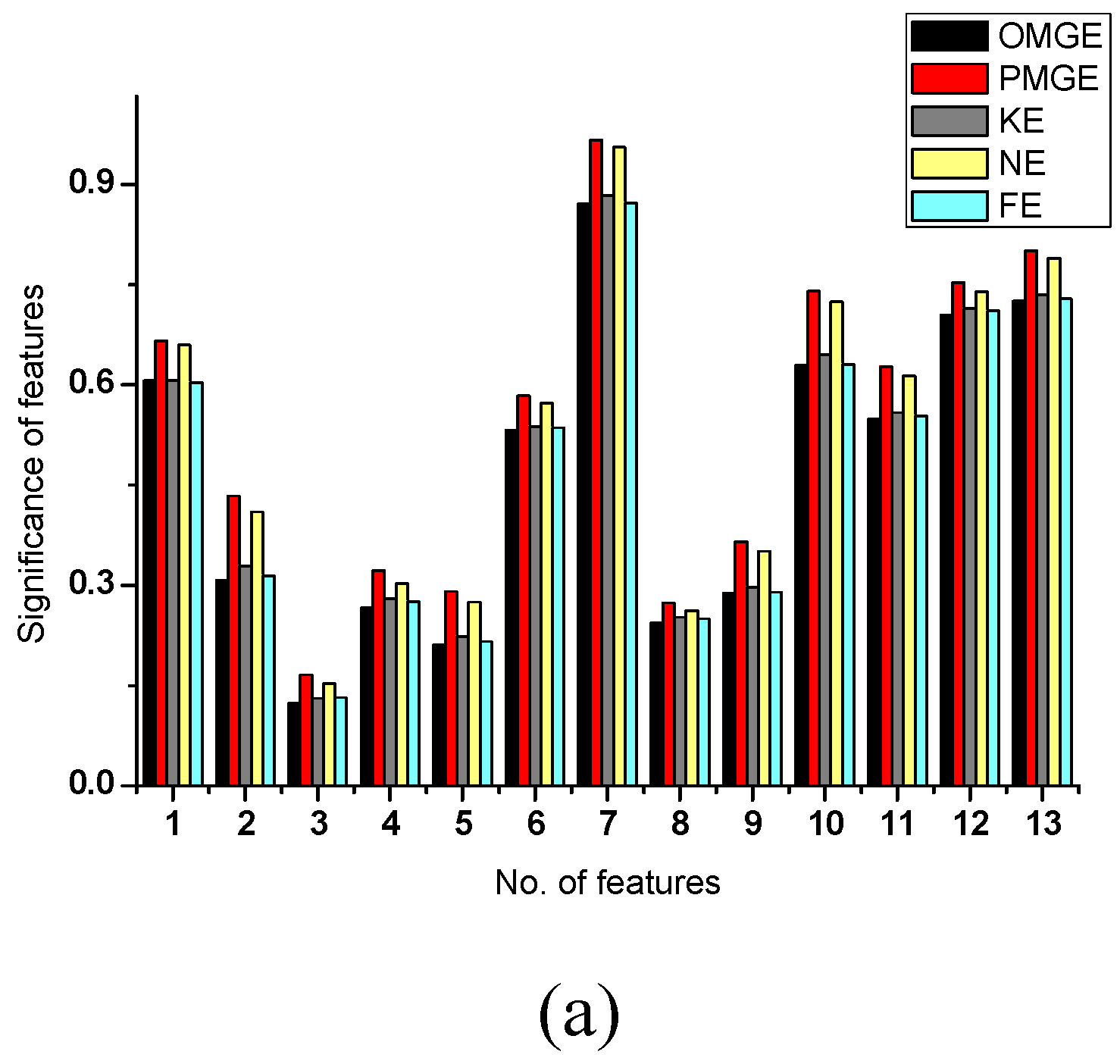
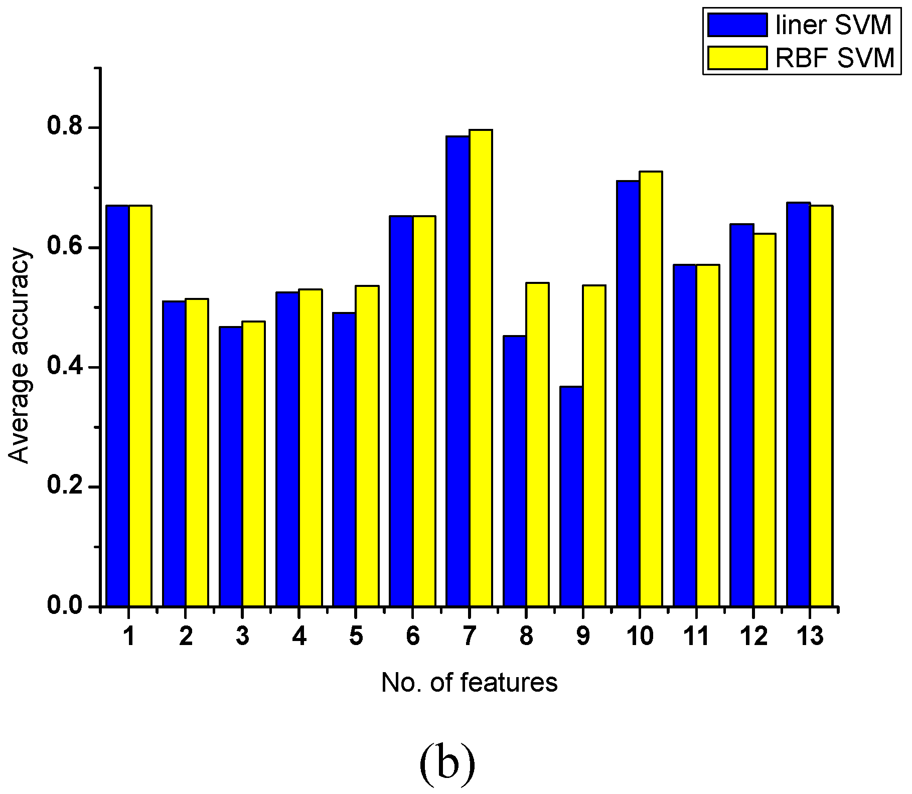
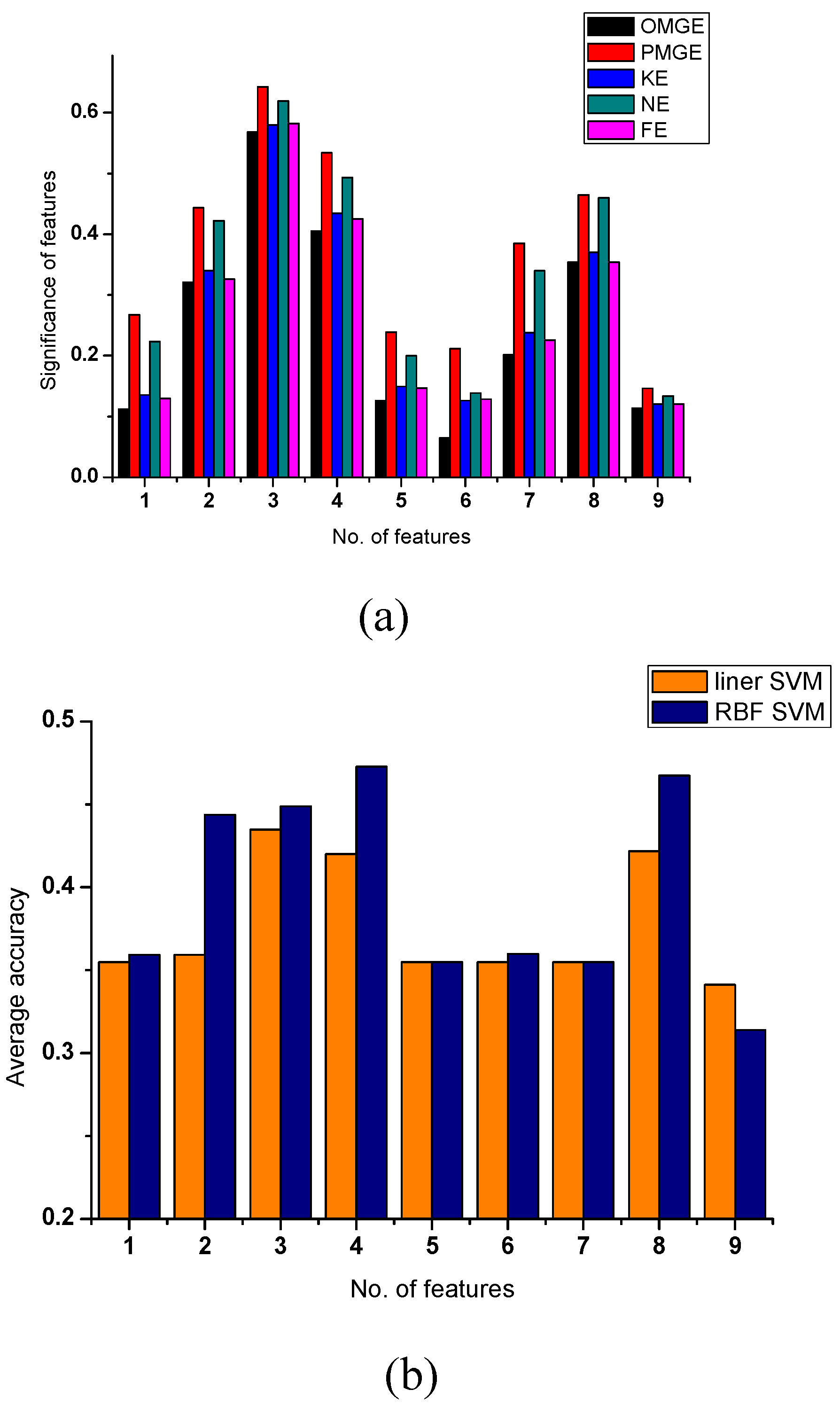
Two data sets wine and glass are used in the experiment. There are 13 features in the wine and nine features in the glass dataset. The results are given in Figure 1 and Figure 2. As to the wine data, the features 1, 6, 7, 10, 11, 12, 13 produce higher values of all evaluation functions, as shown in Figure 1a; at the same time, we can also find that the classification accuracies of these features are better than others (again shown in Figure 1b). As to the glass data, features 2, 3, 4, 8 are better than others in terms of the five evaluating functions, corresponding the classification accuracies of features 2, 3, 4, 8 are also higher than the other features. These results show that all five evaluating functions can produce good estimates of classification ability of the features. It can be concluded that OMGE and PMGE are competent with other entropy models.

Figure 1. Significance and accuracy of single feature (wine). (a) Significance of a single feature computed with different evaluating. (b) Classification accuracies obtained for single features when using linear SVM and RBF SVM.

Figure 1. Significance and accuracy of single feature (wine). (a) Significance of a single feature computed with different evaluating. (b) Classification accuracies obtained for single features when using linear SVM and RBF SVM.

Figure 2. Significance and accuracy of single feature(glass). (a) Significance of a single feature computed with different evaluating. (b) Classification accuracies obtained for single features when using linear SVM and RBF SVM.

Figure 2. Significance and accuracy of single feature(glass). (a) Significance of a single feature computed with different evaluating. (b) Classification accuracies obtained for single features when using linear SVM and RBF SVM.

The above results show MGE can be used to evaluate single attributes. Now, we show the effectiveness in attribute reduction. The selected features with different algorithms are presented in Table 3 and Table 4, respectively. Regarding OMGE, PMGE, FE, NE and KE, the orders of the features presented in the tables are the orders that the features are kept being added to the feature space. These orders reflect the relative significance of features in terms of the corresponding measures. Some results can be derived from the selected attributes. First, whatever attribute selection techniques have been used, most of the attributes in all datasets can be deleted. The reduction rate is high to 90% for some datasets, such as sonar and wpbc. Second, some selected attributes are slightly different. Especially, some of the selected features are the subset of attributes selected by other models.

Table 3. Subsets of features selected with OMGE and PMGE.

Data	OMGE	PMGE
wine	7,1,10,13	7,1,11,4
wdbc	29,22,23,12,9	24,29,23,30,26,9,13,10,28,3,27
iono	5,6,8,25,28,24,10,21	5,6,34,29,8,23
heart	13,12,3,11,1,7,4	13,12,3,1,10,4
glass	3,7,4,9,5	3,7,4,9,5,1
wpbc	34,2,13,14,7	2,34,13,7,23
sonar	12,27,21,37,32,30,54	12,16,26,40,48

Table 3. Subsets of features selected with OMGE and PMGE.

Data	OMGE	PMGE
wine	7,1,10,13	7,1,11,4
wdbc	29,22,23,12,9	24,29,23,30,26,9,13,10,28,3,27
iono	5,6,8,25,28,24,10,21	5,6,34,29,8,23
heart	13,12,3,11,1,7,4	13,12,3,1,10,4
glass	3,7,4,9,5	3,7,4,9,5,1
wpbc	34,2,13,14,7	2,34,13,7,23
sonar	12,27,21,37,32,30,54	12,16,26,40,48

Table 4. Subsets of features selected with FE, NE and KE.

Data	FE	NE	KE
wine	7, 1, 10,13	7,1,11,4	7,1,10,13
wdbc	29,22,23,12,9	24,29,23,30,8,27,26,13,10,3,19	29,22,23,9,12
iono	5,6,8,25,28,24,34,7	5,6,34,29,8,23	5,6,8,25,28,24,34,7
heart	13,12,3,10,1,7,11,2,8,4	13,12,3,10,1,4,5	13,12,3,10,1,7,11
glass	3,7,4,9,5	3,7,4,9,5,1	3,7,4,9,5
wpbc	34,2,13,14,7	2,34,13,7,23	34,2,13,14,7
sonar	12,27,21,37,32,30,54	12,16,26,40,48	12,16,26,37,22,32,28

Table 4. Subsets of features selected with FE, NE and KE.

Data	FE	NE	KE
wine	7, 1, 10,13	7,1,11,4	7,1,10,13
wdbc	29,22,23,12,9	24,29,23,30,8,27,26,13,10,3,19	29,22,23,9,12
iono	5,6,8,25,28,24,34,7	5,6,34,29,8,23	5,6,8,25,28,24,34,7
heart	13,12,3,10,1,7,11,2,8,4	13,12,3,10,1,4,5	13,12,3,10,1,7,11
glass	3,7,4,9,5	3,7,4,9,5,1	3,7,4,9,5
wpbc	34,2,13,14,7	2,34,13,7,23	34,2,13,14,7
sonar	12,27,21,37,32,30,54	12,16,26,40,48	12,16,26,37,22,32,28

As we know, we consider the ranking of features in feature selection, sometimes, a little difference in feature qualities may lead to completely different ranking. Therefore, the great difference between these selected features is the difference between the qualities of features computed with diverse granularities. In other words, there is a inconsistent relationship between its values under one-granularity and those under the another granularity. In [7], the authors give a tentative study that multi-granulation model will display its advantage for rule extraction when two granularities process a contradiction relationship. We will test this idea by the following experiment. We build classification models with the selected features and test their classification performance based on 10-fold cross validation. The average value and standard deviation are used to measure the classification performance. We compare the raw data, MGE, FE, NE and KE in Table 5, Table 6 and Table 7, where learning algorithms CART, linear SVM and RBF SVM are introduced to evaluate the selected features.

Table 5. Classification accuracies based on CART (%).

Data	Raw data	OMGE	PMGE	FE	NE	KE
wine	86.4 ± 7.9	92.2 ± 7.5	89.9 ± 8.5	92.2 ± 7.5	89.9 ± 8.5	92.2 ± 7.5
wdbc	90.3 ± 6.0	93.0 ± 3.8	93.5 ± 3.9	93.0 ± 3.8	94.0 ± 3.2	93.0 ± 3.8
iono	86.4 ± 7.2	87.5 ± 5.6	88.6 ± 6.5	88.1 ± 6.0	88.6 ± 6.5	88.1 ± 6.0
heart	77.0 ± 5.5	78.5 ± 7.3	80.4 ± 9.0	75.2 ± 9.2	80.0 ± 7.7	77.8 ± 9.2
glass	69.2 ± 13.2	65.7 ± 12.9	65.1 ± 14.6	65.7 ± 12.9	65.1 ± 14.6	65.7 ± 12.9
wpbc	70.2 ± 5.4	70.7 ± 10.3	71.1 ± 11.9	70.7 ± 10.3	71.1 ± 11.9	70.7 ± 10.3
sonar	57.7 ± 9.2	73.1 ± 12.6	72.2 ± 15.3	73.1 ± 12.6	72.2 ± 15.3	62.6 ± 13.2

Table 5. Classification accuracies based on CART (%).

Data	Raw data	OMGE	PMGE	FE	NE	KE
wine	86.4 ± 7.9	92.2 ± 7.5	89.9 ± 8.5	92.2 ± 7.5	89.9 ± 8.5	92.2 ± 7.5
wdbc	90.3 ± 6.0	93.0 ± 3.8	93.5 ± 3.9	93.0 ± 3.8	94.0 ± 3.2	93.0 ± 3.8
iono	86.4 ± 7.2	87.5 ± 5.6	88.6 ± 6.5	88.1 ± 6.0	88.6 ± 6.5	88.1 ± 6.0
heart	77.0 ± 5.5	78.5 ± 7.3	80.4 ± 9.0	75.2 ± 9.2	80.0 ± 7.7	77.8 ± 9.2
glass	69.2 ± 13.2	65.7 ± 12.9	65.1 ± 14.6	65.7 ± 12.9	65.1 ± 14.6	65.7 ± 12.9
wpbc	70.2 ± 5.4	70.7 ± 10.3	71.1 ± 11.9	70.7 ± 10.3	71.1 ± 11.9	70.7 ± 10.3
sonar	57.7 ± 9.2	73.1 ± 12.6	72.2 ± 15.3	73.1 ± 12.6	72.2 ± 15.3	62.6 ± 13.2

Table 6. Classification accuracies based on liner SVM (%).

Data	Raw data	OMGE	PMGE	FE	NE	KE
wine	98.3 ± 2.7	97.2 ± 3.9	94.4 ± 5.2	97.2 ± 3.9	94.4 ± 5.2	97.2 ± 3.9
wdbc	98.0 ± 1.9	96.1 ± 2.1	96.3 ± 2.1	96.1 ± 2.1	95.9 ± 2.1	96.1 ± 2.1
iono	87.5 ± 6.4	83.4 ± 5.3	85.0 ± 5.9	85.0 ± 5.3	85.0 ± 5.9	85.0 ± 5.3
heart	84.1 ± 9.3	83.0 ± 8.9	81.9 ± 7.2	82.9 ± 9.4	82.2 ± 6.0	82.6 ± 8.6
glass	55.7 ± 7.7	60.4 ± 9.1	57.1 ± 8.7	60.4 ± 9.1	57.1 ± 8.7	60.4 ± 9.1
wpbc	77.3 ± 5.7	76.3 ± 3.0	76.3 ± 3.0	76.3 ± 3.0	76.3 ± 3.0	76.3 ± 3.0
sonar	64.4 ± 15.7	64.9 ± 11.6	67.8 ± 15.7	64.9 ± 11.6	67.8 ± 15.7	65.5 ± 13.5

Table 6. Classification accuracies based on liner SVM (%).

Data	Raw data	OMGE	PMGE	FE	NE	KE
wine	98.3 ± 2.7	97.2 ± 3.9	94.4 ± 5.2	97.2 ± 3.9	94.4 ± 5.2	97.2 ± 3.9
wdbc	98.0 ± 1.9	96.1 ± 2.1	96.3 ± 2.1	96.1 ± 2.1	95.9 ± 2.1	96.1 ± 2.1
iono	87.5 ± 6.4	83.4 ± 5.3	85.0 ± 5.9	85.0 ± 5.3	85.0 ± 5.9	85.0 ± 5.3
heart	84.1 ± 9.3	83.0 ± 8.9	81.9 ± 7.2	82.9 ± 9.4	82.2 ± 6.0	82.6 ± 8.6
glass	55.7 ± 7.7	60.4 ± 9.1	57.1 ± 8.7	60.4 ± 9.1	57.1 ± 8.7	60.4 ± 9.1
wpbc	77.3 ± 5.7	76.3 ± 3.0	76.3 ± 3.0	76.3 ± 3.0	76.3 ± 3.0	76.3 ± 3.0
sonar	64.4 ± 15.7	64.9 ± 11.6	67.8 ± 15.7	64.9 ± 11.6	67.8 ± 15.7	65.5 ± 13.5

Table 7. Classification accuracies based on RBF SVM (%).

Data	Raw data	OMGE	PMGE	FE	NE	KE
wine	97.8 ± 2.9	96.7 ± 3.9	95.0 ± 4.1	96.7 ± 3.9	95.0 ± 4.1	96.7 ± 3.9
wdbc	97.0 ± 2.6	96.7 ± 2.1	97.2 ± 2.3	96.7 ± 2.1	97.5 ± 2.5	96.7 ± 2.1
iono	94.0 ± 4.2	93.7 ± 4.8	92.6 ± 5.7	94.0 ± 4.6	92.6 ± 5.7	94.0 ± 4.6
heart	79.2 ± 9.6	81.1 ± 7.9	83.3 ± 7.6	82.6 ± 9.4	84.0 ± 7.8	81.5 ± 9.2
glass	68.3 ± 12.1	62.7 ± 11.9	64.1 ± 11.2	62.7 ± 11.9	64.1 ± 11.2	62.7 ± 11.9
wpbc	78.9 ± 6.0	74.3 ± 7.4	75.3 ± 7.7	74.3 ± 7.4	75.3 ± 7.7	74.3 ± 7.4
sonar	58.5 ± 16.0	65.9 ± 14.9	64.1 ± 11.2	65.9 ± 14.9	64.1 ± 11.2	61.1 ± 7.2

Table 7. Classification accuracies based on RBF SVM (%).

Data	Raw data	OMGE	PMGE	FE	NE	KE
wine	97.8 ± 2.9	96.7 ± 3.9	95.0 ± 4.1	96.7 ± 3.9	95.0 ± 4.1	96.7 ± 3.9
wdbc	97.0 ± 2.6	96.7 ± 2.1	97.2 ± 2.3	96.7 ± 2.1	97.5 ± 2.5	96.7 ± 2.1
iono	94.0 ± 4.2	93.7 ± 4.8	92.6 ± 5.7	94.0 ± 4.6	92.6 ± 5.7	94.0 ± 4.6
heart	79.2 ± 9.6	81.1 ± 7.9	83.3 ± 7.6	82.6 ± 9.4	84.0 ± 7.8	81.5 ± 9.2
glass	68.3 ± 12.1	62.7 ± 11.9	64.1 ± 11.2	62.7 ± 11.9	64.1 ± 11.2	62.7 ± 11.9
wpbc	78.9 ± 6.0	74.3 ± 7.4	75.3 ± 7.7	74.3 ± 7.4	75.3 ± 7.7	74.3 ± 7.4
sonar	58.5 ± 16.0	65.9 ± 14.9	64.1 ± 11.2	65.9 ± 14.9	64.1 ± 11.2	61.1 ± 7.2

Comparing the performance of raw data and granulation-based selection, we can find although most of features have been removed, most of the classification accuracies derived from the reduced data sets do not decrease, but increase. It shows there are redundant and irrelevant attributes in the raw data.

The experimental results show that no matter which classification algorithms are used, MGE is better than or equivalent to KE. Table 6 shows that MGE outperforms FE and NE with respect to liner SVM. As to CART learning algorithm in Table 5, MGE is better than or equivalent to NE for six of the seven databases. It can be concluded that MGE is a better choice for the diverse granularities. Actually, the different decision makers have different granulation points of view. Therefore, it is necessary to take diverse factors into consideration for granular computing in the real world.

6. Conclusions

In this paper, the classical single-granulation entropy theory has been extended. As a result of this extension, a multi-granulation entropy model (MGE) has been developed. The uncertainty of the information system is defined by using multiple relations on the universe. These relations can be chosen according to a user’s requirements or targets of problem solving.

In MGE model, we introduce OMGE and PMGE to describe the relations between different granularities. Based on the mutual information defined through MGE, we proposed the forward greed features selection algorithms, which will be helpful for applying this theory to practical issues. MGE provides an effective approach in the context of multiple granulations. We conclude that the single-granulation entropy is the special instance of MGE. The experimental result shows that MGE will display its advantage for rule extraction and knowledge discovery when the different granularities in information systems possess a contradiction or inconsistent relationship.

The future work could move along two directions. First, the existing feature selection algorithms based entropy sometimes might not be robust enough for real-world applications. How to improve it is an important issue. Second, we will continue to construct MGE models with various binary relations for discussing the common properties of this kind of entropy model.

References

- Knuth, K.H. Lattice duality: The origin of probability and entropy. Neurocomputing 2005, 67, 245–274. [Google Scholar] [CrossRef]
- Harremoës, P.; Vajda, I. On the bahadur-efficient testing of uniformity by means of the entropy. IEEE Trans. Inform. Theory 2008, 54, 321–331. [Google Scholar] [CrossRef]
- Santhanam, N.P.; Modha, D. Lossy Lempel-Ziv like compression algorithms for memoryless sources. In Proceedings of 49th Annual Allerton Conference, Monticello, IL, USA, 28–30 September 2011; pp. 1751–1756.
- Yu, D.R.; Hu, Q.H.; Wu, C.X. Uncertainty measures for fuzzy relations and their applications. Appl. Soft Comput. 2007, 7, 1135–1143. [Google Scholar] [CrossRef]
- Hu, Q.H.; Zhang, L.; Chen, D.G.; Pedrycz, W.; Yu, D.R. Gaussian kernel based fuzzy rough sets: model, uncertainty measures and applications. Int. J. Approx. Reason. 2010, 51, 453–471. [Google Scholar] [CrossRef]
- Hu, Q.H.; Zhang, L.; Zhang, D.; Pan, W.; An, S.; Pedrycz, W. Measuring relevance between discrete and continuous features based on neighborhood mutual information. Expert Syst. Appl. 2011, 38, 10737–10750. [Google Scholar] [CrossRef]
- Qian, Y.H.; Liang, J.Y.; Yao, Y.Y.; Dang, C.Y. MGRS: A multi-granulation rough set. Inform. Sci. 2010, 180, 949–970. [Google Scholar] [CrossRef]
- Lin, G.P.; Li, J.J. A covering-based pessimistic multigranulation rough set. In Proceedings of International Conference on Intelligent Computing, Zhengzhou, China, 11–14 August, 2011; pp. 673–680.
- Xu, W.H.; Zhang, X.T.; Wang, Q.R. A generalized multi-granulation rough set approach. In Proceedings of International Conference on Intelligent Computing, Zhengzhou, China, 11–14 August, 2011; pp. 681–689.
- Qin, K.Y.; Yang, J.L.; Pei, Z. Generalized rough sets based on reflexive and transitive relations. Inform. Sci. 2008, 178, 4138–4141. [Google Scholar] [CrossRef]
- Zhu, W.; Wang, S.P. Rough matroids based on relations. Inform. Sci. 2013, 232, 241–252. [Google Scholar] [CrossRef]
- Tang, J.G.; She, K.; Min, F.; Zhu, W. A matroidal approach to rough set theory. Theor. Comput. Sci. 2013, 471, 1–11. [Google Scholar] [CrossRef]
- Jing, S.Y.; She, K.; Ali, S. A Universal neighbourhood rough sets model for knowledge discovering from incomplete heterogeneous data. Expert Syst. 2013, 30, 89–96. [Google Scholar] [CrossRef]
- Al-Sharhan, S.; Karray, F.; Gueaieb, W.; Basir, O. Fuzzy entropy: a brief survey. In The 10th IEEE International Conference on Fuzzy Systems; IEEE: Melbourne, Australia, 2001; Volume 3, pp. 1135–1139. [Google Scholar]
- Hu, Q.H.; Yu, D.R. Neighborhood Entropy. In Proceedings of the Eighth International Conference on Machine Learning and Cybernetics, Baoding, China, 12–15 July 2009; Volume 3, pp. 1776–1782.
- Wang, G.Y. Rough reduction in algebra view and information view. Int. J. Intell. Syst. 2003, 18, 679–688. [Google Scholar] [CrossRef]
- Slezak, D. Approximate entropy reducts. Fund. Informat. 2002, 53, 365–390. [Google Scholar]
- Hu, Q.H.; Yu, D.R.; Xie, Z.X.; Liu, J.F. Fuzzy probabilistic approximation spaces and their information measures. IEEE Trans. Fuzzy Syst. 2006, 14, 191–201. [Google Scholar]
- Yu, L.; Liu, H. Efficient feature selection via analysis of relevance and redundancy. J. Mach. Learn. Res. 2004, 5, 1205–1224. [Google Scholar]
- Battiti, R. Using mutual information for selecting features in supervised neural net learning. IEEE T. Neural Networ. 1994, 5, 537–550. [Google Scholar] [CrossRef] [PubMed]
- Dash, M.; Liu, H. Consistency-based search in feature selection. Artif. Intell. 2003, 151, 155–176. [Google Scholar] [CrossRef]
- Muni, D.P.; Pal, N.R.; Das, J. Genetic programming for simultaneous feature selection and classifier design. IEEE T. Syst. Man. Cy. B 2006, 36, 106–117. [Google Scholar] [CrossRef]
© 2013 by the authors; licensee MDPI, Basel, Switzerland. This article is an open access article distributed under the terms and conditions of the Creative Commons Attribution license (http://creativecommons.org/licenses/by/3.0/).
Share and Cite
MDPI and ACS Style
Zeng, K.; She, K.; Niu, X. Multi-Granulation Entropy and Its Applications. Entropy 2013, 15, 2288-2302. https://doi.org/10.3390/e15062288
AMA Style
Zeng K, She K, Niu X. Multi-Granulation Entropy and Its Applications. Entropy. 2013; 15(6):2288-2302. https://doi.org/10.3390/e15062288
Chicago/Turabian StyleZeng, Kai, Kun She, and Xinzheng Niu. 2013. "Multi-Granulation Entropy and Its Applications" Entropy 15, no. 6: 2288-2302. https://doi.org/10.3390/e15062288