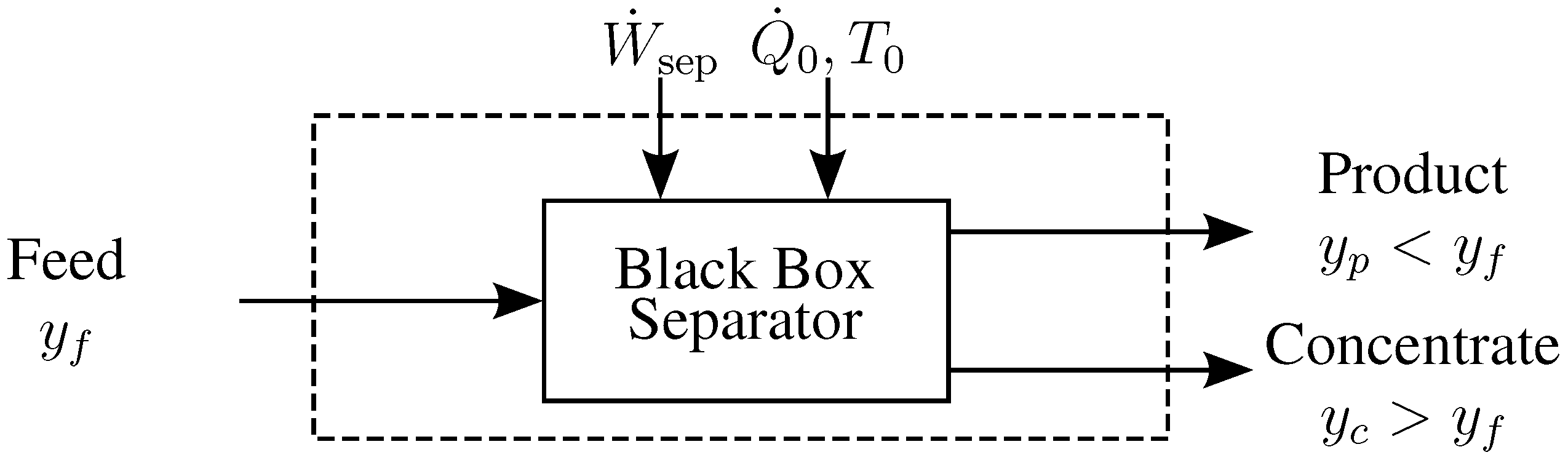
In order to illustrate the application of Equations (23) and (24), energetic and economic analysis of several desalination systems are considered. First, a simplified calculation of and is performed for a multistage flash (MSF) plant and an MED plant using cost data available in the literature coupled with some simple approximations. Second, a much more detailed analysis of an RO system is performed in which the energetics are modeled by evaluating all of the irreversibilities in the system. The energetic model is coupled with a full cost model in order to show how economic costs are influenced by energetics. Third, a complete energetic and economic model of a solar powered direct contact membrane distillation (DCMD) is analyzed in order to demonstrate how systems powered using “free” energy should be studied.
4.1. Multistage Flash and Multiple Effect Distillation
MSF and MED are the two most common thermal desalination technologies [
20]. Both are distillation methods in which the overall energy requirements are reduced through the use of energy recovery in each stage or effect of the system [
21]. Cost information for representative 100,000 m
3/d MSF and MED plants is provided by [
22,
23,
24,
25,
26]. It is shown that the total cost of water production for the MSF and MED plants is $0.89/m
3 and $0.72/m
3. A breakdown of the costs is provided in
Table 1. Additionally, the thermal and electrical energy requirements are provided.
Table 1.
Breakdown of costs for a 100,000 m
3/d multistage flash (MSF) and multiple effect distillation (MED) system [
22].
Table 1.
Breakdown of costs for a 100,000 m3/d multistage flash (MSF) and multiple effect distillation (MED) system [22].
| MSF | MED |
|---|
| Costs [$/m3]: |
| Amortization | 0.29 | 0.22 |
| Maintenance | 0.01 | 0.01 |
| Chemical | 0.05 | 0.08 |
| Labor | 0.08 | 0.08 |
| Thermal energy | 0.27 | 0.27 |
| Electrical energy | 0.19 | 0.06 |
| Total | 0.89 | 0.72 |
| Energy requirements: |
| Thermal energy [kWht/m3] | 78 | 69 |
| Electrical energy [kWhe/m3] | 4.0 | 1.0 |
Using the information in
Table 1, it is possible to calculate both
and
as well as to compare all of the contributions to the total cost of producing water for the two systems provided some additional assumptions are made. The feed is assumed to be standard seawater at 25 °C and 35 g/kg [
27,
28] while the steam temperature is assumed to be 100 °C. Note that the minimum least heat of separation is a function of steam temperature, so the exact values found in the following calculation are subject to change based on the actual (but unreported) steam temperature. However, since this example is used to demonstrate a methodology, rather than to draw significant comparisons between the two plants, this broad approximation is deemed acceptable. Finally, it is assumed that thermal energy is the primary energy input to the system. While MSF and MED plants are typically operated in cogeneration schemes, without further information, it is not possible to characterize the actual conversion efficiencies involved in the cogeneration power plant [
4].
Using the generalized least energy of separation equation from Mistry and Lienhard [
4]:
the least heat of separation is equal to the least work of separation divided by Carnot efficiency. Using Equation (2) and a standard seawater property package [
27,
28], the minimum least heat of separation for seawater using a steam temperature of 100 °C is 13.5 kJ/kg (3.7 kWh
t/m
3) [
22].
The price of both the thermal and electrical energy is evaluated by dividing the cost by the energy requirements. Note that the cost of energy is heavily dependent on location and source. Therefore, it is not expected that the cost of heat and electricity will be the same for the two plants considered. For MSF, this corresponds to heat and electricity prices of $0.0034kWht and $0.0467kWhe, respectively. For MED, this corresponds to $0.0040kWht and $0.0576kWhe.
Finally, the total energy input for both systems is equal to the sum of the exergies of the heat and work. Expressed in terms of heat (i.e., ), the effective thermal input to the MSF and MED systems is 97.9kWht/m3 and 74.0kWht/m3, respectively. Using these values coupled with the minimum least heat of separation, for the MSF and MED plants is 3.8% and 5.1%, respectively.
Similarly,
can be evaluated by multiplying the price of the primary energy (heat for thermal systems) and the minimum least heat of separation and dividing the result by the total cost of water production. Using the prices for heat determined above,
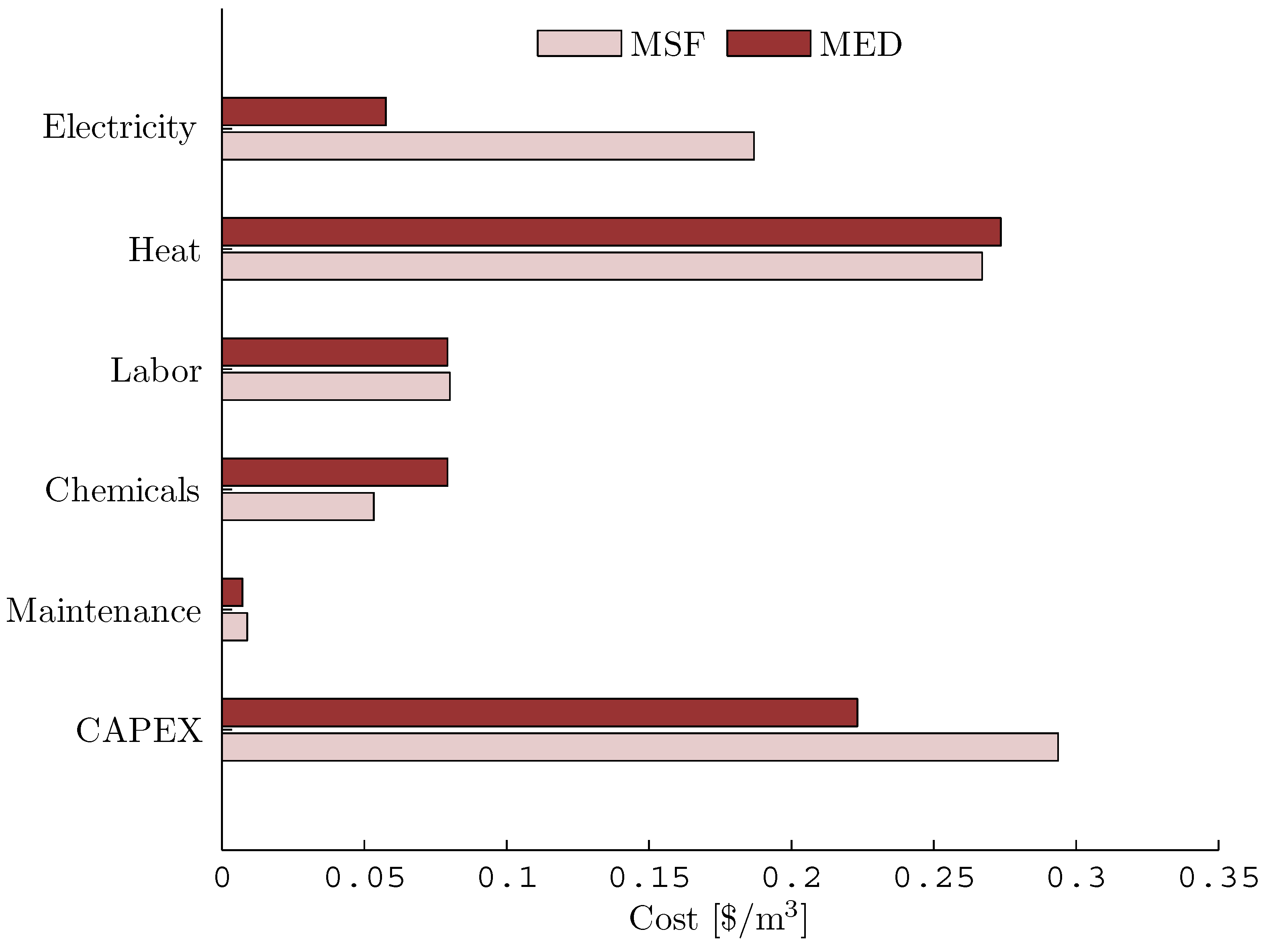
for the MSF and MED plants is evaluated to be 1.4% and 2.1%, respectively. The specific breakdown of the costs, as shown in
Table 1, is shown in
Figure 2.
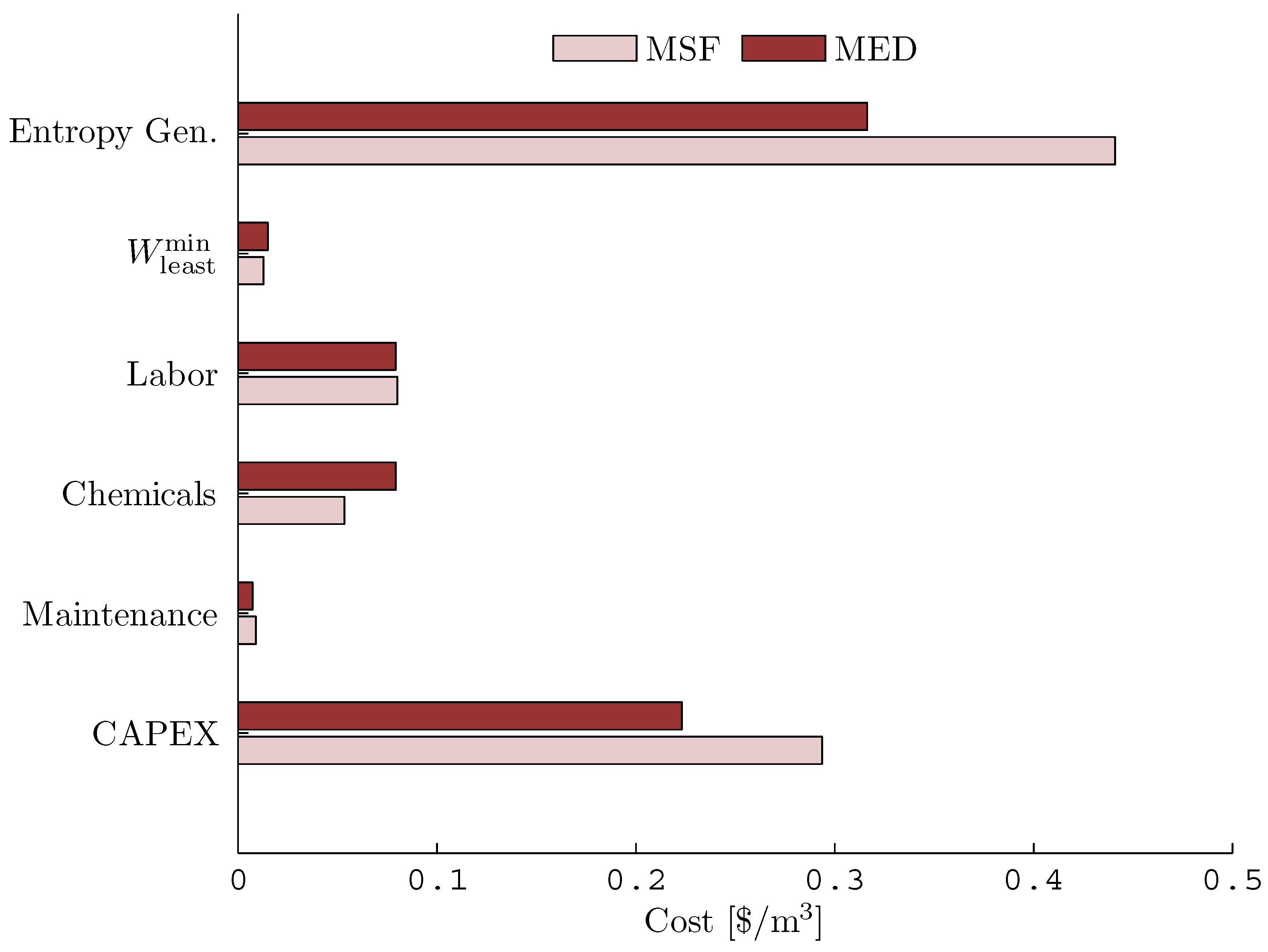
The values of
found above are evaluated using Equation (23). If instead, Equation (24) is used, then the cost of the energetic input can be split into the cost of providing the minimum least heat of energy plus the sum of the costs of providing extra energy required to account for all of the thermodynamic irreversibilities. The results are shown in
Figure 3.
From
Figure 3, it is clear that the cost of excess energy required by the irreversibilities is the single greatest source of the total cost of producing water for these two representative MSF and MED plants. Given more detailed information about the systems in question, the irreversibilities could be further subdivided in order to isolate the specific source of loss. Then, a system designer could identify which components or processes should be addressed in order to try to reduce the overall system cost.
At this point, it should be reiterated that these are just representative numbers and that these two examples (and the following examples) are not meant to be used to draw sweeping conclusions about the superiority of one technology over another.
Figure 2.
Breakdown of costs associated with the production of water using MSF and MED.
Figure 2.
Breakdown of costs associated with the production of water using MSF and MED.
Figure 3.
Breakdown of costs associated with the production of water using MSF and MED with entropy generation isolated.
Figure 3.
Breakdown of costs associated with the production of water using MSF and MED with entropy generation isolated.
In the next section, an energetic and economic model for a reverse osmosis system is presented and studied in greater detail than was possible based on the information available for the MSF and MED systems. By using an energetic model, specific sources of irreversibilities for the RO system are isolated.
4.2. Reverse Osmosis
Reverse osmosis is the most common form of desalination [
20]. A representative flow path of a single stage RO plant with energy recovery is shown in
Figure 4 [
29]. A simple model based on the pressure differences throughout the system is used to evaluate the energetic requirements of this system [
3]. In order to simplify the analysis of this system, thermal effects are neglected since they are of second order to pressure effects. Additionally, several approximations and design decisions are made.
Figure 4.
A typical flow path for a single stage reverse osmosis system [
3].
Figure 4.
A typical flow path for a single stage reverse osmosis system [
3].
Feed seawater enters the system at ambient conditions (25 °C, 1 bar, 35 g/kg salinity). The product is pure H
2O (0 g/kg salinity) produced at a recovery ratio of 40%. In order to match flow rates in the pressure exchanger, 40% of the feed is pumped to 69 bar using a high pressure pump while the remaining 60% is pumped to the same pressure using a combination of a pressure exchanger driven by the rejected brine as well as a booster pump. All pumps are assumed to have isentropic efficiencies of 85%. The concentrated brine loses 2 bar of pressure through the RO module while the product leaves the module at 1 bar. Energy Recovery Inc. (ERI) [
30] makes a direct contact pressure exchanger that features a single rotating part. The pressure exchanger pressurizes part of the feed using work produced through the depressurization of the brine in the rotor. Assuming that the expansion and compression processes are 98% efficient [
3,
30], the recovered pressure is calculated as follows:
and the pressure exchanger efficiency is evaluated using ERI’s definition [
29]:
Density of seawater is evaluated using standard seawater properties [
27,
28].
Mistry
et al. [
3] derived simple formulas based on the ideal gas and incompressible fluid models for the entropy generation through various mechanisms found in desalination processes. Entropy generated in the high pressure pump, booster pump, and the feed in the pressure exchanger is given by:
where
c is the specific heat,
v is the specific volume,
is the isentropic efficiency of the pump, and states 1 and 2 correspond to the inlet and outlet, respectively. Similarly, entropy generated through the expansion of the pressurized brine in the pressure exchanger is given by:
where
is the isentropic efficiency of the expansion device.
Entropy generation in the RO module is a function of the change of both the mechanical and chemical states of seawater. In order to evaluate entropy generation, the change in entropy associated with all parts of the process path must be considered. Given that entropy is a state variable, the process can be decomposed into two sub-processes for the purpose of calculating the overall change of state. First, the high pressure seawater is isobarically and isothermally separated into two streams of different composition (note, in a real system, this would require a heat transfer process with the environment; however, thermal effects are neglected in this analysis). Second, the two streams are depressurized at constant salinity in order to account for the pressure drop associated with diffusion through the membrane (product, bar) and that associated with hydraulic friction (brine, bar).
Entropy change due to the separation process is evaluated as a function of temperature, pressure, and salinity of each of the process streams. For the model of separation considered here, the compositional change is taken at constant high pressure and temperature:
Standard seawater properties [
27,
28] are used for evaluating entropy. Even though this property package is independent of pressure, it may be used because seawater is nearly incompressible resulting in entropy being largely independent of
p.
Mistry
et al. [
3] showed that entropy generation due to the irreversible depressurization of both the brine and product streams is given by:
The total entropy generated in the RO module is the sum of the entropy change due to compositional changes, Equation (31), and the entropy generated in the depressurization of the product and brine streams, Equation (32).
Entropy generated as a result of the discard of disequilibrium streams to the environment must also be considered. Thermal and chemical disequilibrium entropy generation can be evaluated using [
3]:
Since thermal effects are neglected in this analysis, Equation (33) reduces to zero. The energy dissipated by pressure loss and pump inefficiency results in very small increases in the system temperature. As a result, the entropy generation associated with the transfer of this energy out of the system as heat (if any) through the very small temperature difference from the environment is negligible relative to the mechanical sources of entropy production.
Using Equations (27) and (29) to (32) and the denominator of Equation (9), the required energy input to the RO system, as well as the entropy generation within each component can be evaluated. The results of this model are provided in
Table 2 and a discussion is provided by Mistry
et al. [
3].
Table 2.
Contributions to the overall energy requirements of a reverse osmosis system, evaluated in terms of entropy generated within each component.
Table 2.
Contributions to the overall energy requirements of a reverse osmosis system, evaluated in terms of entropy generated within each component.
| Sources of | Entropy Generation | Energy Contribution |
|---|
| Energy Consumption | [J/kg K] | [kJ/kg] |
|---|
| - | 2.71 |
| RO Module | 10.6 | 3.16 |
| High pressure pump | 3.87 | 1.15 |
| Pressure exchanger | 1.26 | 0.377 |
| Booster pump | 0.407 | 0.121 |
| Feed pump | 0.145 | 0.043 |
| Chemical disequilibrium | 3.08 | 0.918 |
| Total: | 19.4 | 8.48 (2.35 kWh/m3) |
A basic cost model based on the work of Bilton
et al. [
31,
32] is used to generate an estimate of the total cost of producing water. The total annualized cost (TOTEX) is equal to the sum of the capital expenses (CAPEX) and the operating expenses (OPEX) [
6,
12,
33]:
It is typically more convenient to refer to the unit cost of producing water than the annual cost of the system. Cost per unit water can be evaluated by dividing the annualized cost by the yearly water production:
Yearly water production is equal to the daily capacity times the number of days in a year times the availability factor (
):
The CAPEX for a standard RO plant is subdivided into the cost of the RO system and the infrastructure:
The RO system is composed of the RO components, pre-treatment, post-treatment and piping:
The RO components include membranes, pressure vessels, pumps, motors, energy recovery devices (ERD), and connections:
Costs for the components are given in
Table 3. The booster pump and motor are approximated as costing one third the cost of the high pressure pump and motor [
34]. Total component costs are based on a system size of
m
3/d.
Table 3.
Cost of components required for a reverse osmosis system. The number required is determined for a 10,000 m
3/d system, based on the volumetric flow rate capacity of each device. Cost of replacement is considered separately in
Table 5. ERD, energy recovery device.
Table 3.
Cost of components required for a reverse osmosis system. The number required is determined for a 10,000 m3/d system, based on the volumetric flow rate capacity of each device. Cost of replacement is considered separately in Table 5. ERD, energy recovery device.
| Component | Cost | Capacity | Number | Total Cost |
|---|
| [$] | [m3/d] | [-] | [$] |
|---|
| Membrane [35,36] | 550 | 25 | 1,000 | 550,000 |
| Pressure vessel (6 membranes) [37,38] | 1,945 | - | 167 | 325,000 |
| High Pressure pump [39,40] | 50,000 | 720 | 14 | 700,000 |
| Booster pump [34] | 17,000 | 1,000 | 15 | 255,000 |
| High pressure motor [41] | 12,000 | - | 14 | 168,000 |
| Booster motor [34] | 4,000 | - | 15 | 60,000 |
| ERD [34,36,42] | 24,000 | 1,000 | 15 | 360,000 |
| Total () | | | | 2,420,000 |
For typical RO systems, both pre- and post-treatment are needed. Pre-treatment is used to provide basic filtration and treatment to remove large debris, biological contaminants, and other suspended solids that might damage the RO membranes [
43]. Similarly, post-treatment is needed to add essential minerals back to the water so that the water can safely be added to municipal pipelines [
43]. In order to simplify the analysis in this model, both the pre- and post-treatment costs are assumed to be proportional to the total cost of the RO components. Post-treatment costs can also include the cost of storage.
Values for
and
are taken to be 0.35 and 0.03, respectively [
44]. For large municipal-scale systems, it is assumed that the water is fed directly to the water grid and that storage costs may be neglected.
In addition to the cost of the RO plant, there are a number of costs associated with infrastructure. These costs include: land, intake and brine dispersion systems, connections to the grid, installation and construction,
etc. As with the pre- and post-treatments, for simplicity, it is assumed that these costs scale linearly with the cost of the RO plant:
where
is taken to be 1.71 [
44]. Given that infrastructure costs are a significant fraction of the total cost of the system, accurate cost calculations are dependent on the value of
; therefore, this value should always be refined based on the specific plant being considered.
Now that all of the CAPEX are accounted for, they must be converted to annualized costs. This is done by multiplying the CAPEX by an amortization factor, given by:
where
i is the annual interest rate and
n is the expected plant life in years [
45]. For this analysis, a 7.5% interest rate for a plant with a 25 year expected lifetime is assumed [
5]. All capital expenses are summarized in
Table 4. Note that replacement is considered separately in
Table 5.
Table 4.
Summary of capital expenses for a representative reverse osmosis system.
Table 4.
Summary of capital expenses for a representative reverse osmosis system.
| Capital Expenses | Scaling Factor | | Cost [$] |
|---|
| RO Components () | | | 2,420,000 |
| Piping and connections [12] | 0.66 | | 1,600,000 |
| Pre-treatment [44] | 0.35 | | 846,000 |
| Post-treatment [44] | 0.03 | | 72,500 |
| Total RO () | | | 4,930,000 |
| Infrastructure [44] | 1.71 | | 8,430,000 |
| Total Plant () | | | 13,400,000 |
| Annualized CAPEX | 7.5%, 25 years | | 1,200,000 |
| Per m3 | | | 0.346 |
Total OPEX is composed of the costs of labor, chemicals, power, and replacements. Labor, chemicals, and power all scale with the yearly water production,
. If it is assumed the system operates 95% of the time (
), then the costs of labor, chemicals, and power are:
where
is the specific operating cost of labor,
is the average cost of chemicals,
is the cost of electricity, and
is the electricity requirements for the RO system. The electrical requirements for pre- and post-treatment are neglected in this study. For this analysis,
/m
3 [
45,
46] and
/m
3 [
45]. The cost of electricity varies widely depending on location. While the average price for electricity for industrial use in the US is
/kW h, a price more typical of the population-dense areas of the East and West Coasts is closer to
/kW h [
47]. Therefore, the cost of electricity is taken to be
/kW h, while
is evaluated using the RO model described above and summarized in
Table 2 [
3].
Part of the operating expense is the cost of replacing parts as they reach the end of their product lifetime. Given that many components will not last the entire lifetime of the overall plant, it is important to properly account for replacement of expensive components. The annualized cost of replacement is given by:
where
is the annual replacement rate. Values of
along with the corresponding component costs are provided in
Table 5. All OPEX are summarized in
Table 6.
Table 5.
Replacement rate for various reverse osmosis components.
Table 5.
Replacement rate for various reverse osmosis components.
| Component | RR | Ci [$] | Total [$] |
|---|
| Membrane | 0.2 | 550,000 | 110,000 |
| Pumps | 0.1 | 955,000 | 95,500 |
| Motors | 0.1 | 228,000 | 22,800 |
| ERD | 0.1 | 360,000 | 36,000 |
| Pre-treatment | 0.1 | 846,235 | 84,600 |
| Post-treatment | 0.1 | 72,534 | 7,250 |
| Total Replacement Cost () | | | 356,000 |
Table 6.
Summary of operating expenses for a representative reverse osmosis system. OPEX, operating expenses.
Table 6.
Summary of operating expenses for a representative reverse osmosis system. OPEX, operating expenses.
| Operating Expenses | Scaling Factor | | Cost [$] |
|---|
| Labor [45,46] | 0.05 | | 173,000 |
| Chemicals [45] | 0.033 | | 114,000 |
| Electricity [47] | 0.11 | | 899,000 |
| Replacement | | | 356,000 |
| Total Annual OPEX | | | 1,540,000 |
| Per m3 | | | 0.445 |
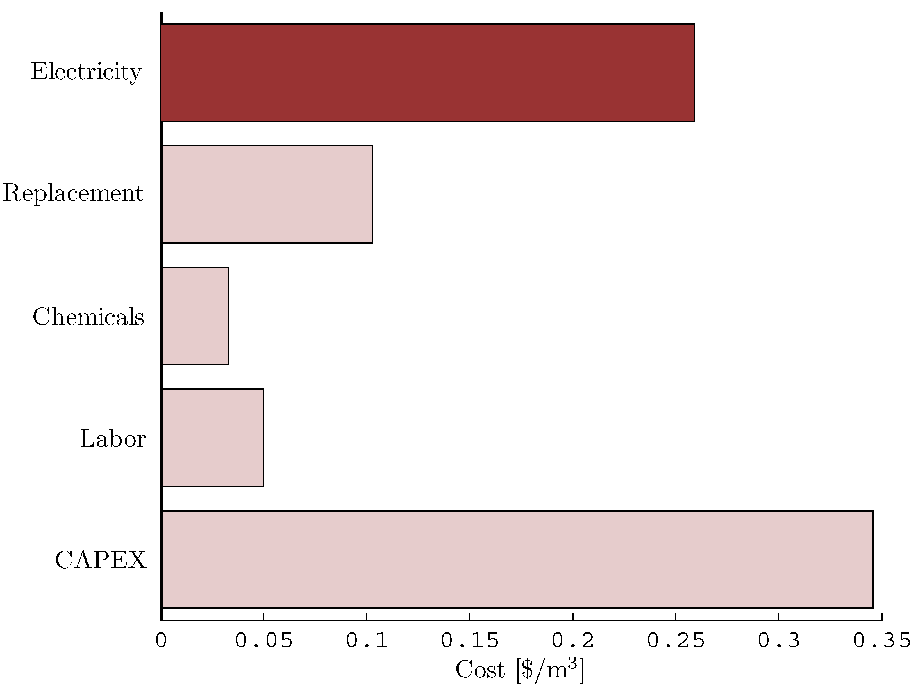
Combining all of the CAPEX and OPEX, an estimate of the cost of water using the RO system shown in
Figure 4 can be evaluated. For a system that produces 10000, the cost of water is estimated to be $0.791/m
3. A bar chart showing the relative contributions to the cost of water production is given in
Figure 5. The economic Second Law efficiency of this system can now be evaluated using Equation (23). Using Equation (2) and a standard seawater property package [
27,
28], the minimum least work of separation for the feed seawater is 2.71 kJ/kg (0.75kWh
e/m
3). Therefore:
Compare this to the value of the Second Law efficiency:
Figure 5.
Breakdown of costs associated with the production of water using reverse osmosis.
Figure 5.
Breakdown of costs associated with the production of water using reverse osmosis.
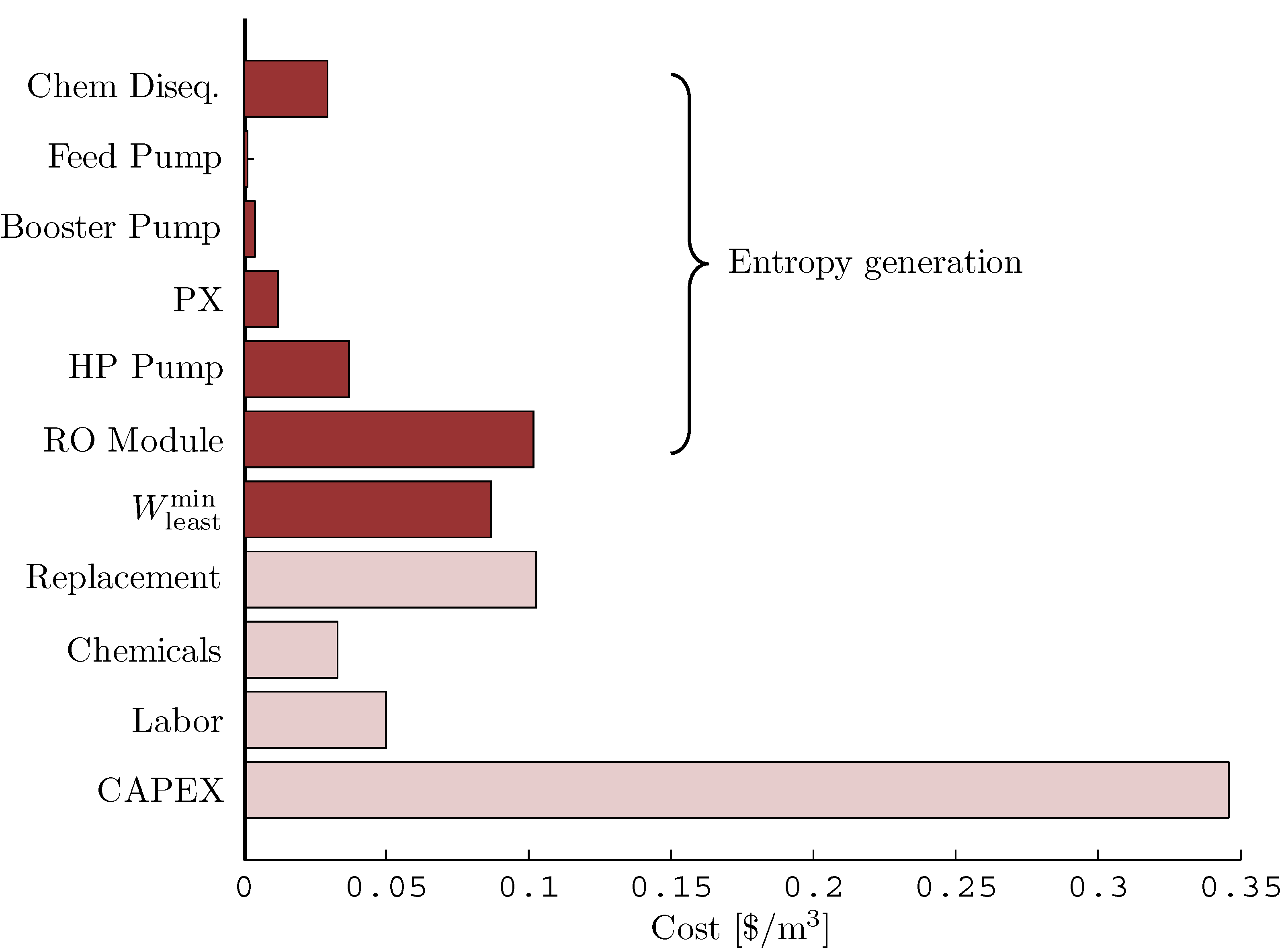
As shown in
Figure 5, costs associated with capital expenses and replacement of parts are the most significant contributors to the overall cost of this particular RO system. However, the cost of energy is also significant and represents about 34% of the overall cost. The overall energy cost can be further subdivided into costs associated with the thermodynamic process of separation (
) and those associated with irreversibilities (
), as shown in
Table 2. Scaling the various energy components using
,
Figure 5 is redrawn in terms of each of the sources of irreversibilities (
Figure 6).
Figure 6 shows that the costs associated with thermodynamic irreversibility are on the same order as the costs associated with replacement costs and the minimum least energy of separation. Irreversibilities associated with losses in the RO module, the high pressure pump and chemical disequilibrium of the brine stream are particularly pronounced. Chemical disequilibrium of the brine is only important in systems in which both the recovery ratio and the Second Law efficiency are high [
3]. Since CAPEX is the greatest source of cost by a wide margin, the system and hardware selection is the most crucial part of the design process. Similarly, replacement cost is a significant contributor to the total cost. This can be reduced by selecting parts with longer lifetimes. In terms of irreversibilities, the energy costs associated with losses in the RO module, the high pressure pump and the chemical energy in the brine are most significant. Losses in the RO module can be reduced through staging and/or batch processing [
48]. Losses in the high pressure (HP) pump can be reduced through the use of higher performance pumps or enhanced energy recovery [
36,
49]. Unfortunately, the irreversibilities associated with the chemical disequilibrium of the concentrate cannot be reduced unless the recovery ratio of the process is reduced.
Figure 6.
Breakdown of costs associated with the production of water using reverse osmosis with the costs of entropy generation isolated by component.
Figure 6.
Breakdown of costs associated with the production of water using reverse osmosis with the costs of entropy generation isolated by component.
Through this analysis, one can clearly see all of the costs associated with the reverse osmosis process and can easily compare the cost of irreversibility in each of the major components. For the particular system seen here, it is clear that CAPEX, and not irreversibility, is the dominant contributor to the total cost of water production.
4.3. Membrane Distillation
Direct contact membrane distillation (DCMD) is a membrane-based thermal distillation process [
50] that can be driven using solar energy. Therefore, it provides a good example for considering the evaluation of
for systems with so-called “free” energy input. In DCMD, a hydrophobic microporous membrane is used to separate the feed and product streams. The temperature difference between a heated feed stream and the cooled fresh water stream induces a vapor pressure difference that drives evaporation through the pores. The vapor diffusion transport process is characterized by the membrane distillation coefficient,
B, a parameter that is used to measure the pore’s diffusion resistance. Experimental DCMD systems have successfully produced fresh water at a small scale (0.1 m
3/d) [
51,
52,
53,
54,
55].
A transport process model for DCMD implemented by Summers
et al. [
55], Saffarini
et al. [
56] is used in this study. A schematic diagram of the system considered is shown in
Figure 7. Key module geometry and constants are shown. The model is based on validated models by Bui
et al. [
57] and Lee
et al. [
54] and was also used by Mistry
et al. [
3] in a previous study. The present calculations are performed for a flat-sheet membrane configuration (Bui
et al. [
57] relied on a hollow-fiber membrane configuration) using membrane geometry and operating conditions typical of pilot-sized plants found in the literature [
58,
59]. Feed seawater (27 °C, 35 g/kg total dissolved solids) enters the system at a mass flow rate of 1 kg/s. The feed is heated to 85 °C using a 90 °C source. In order to balance the mass flow rates through the membrane, the permeate side contains fresh water, also at a flow rate of 1 kg/s. The recovery ratio for this system and operating conditions is 4.4%. A liquid-liquid heat exchanger with a 3 K terminal temperature difference is used to regenerate heat. All pressure drops in the system other than that through the membrane are considered negligible. The pressure drop through the thin channel in the membrane module was found to be the dominant pressure drop in the system and was the basis for calculating the entropy generation due to pumping power. As with the RO model, standard seawater properties are used in this calculation [
27,
28].
Figure 7.
Flow path for a basic direct contact membrane distillation system [
3].
Figure 7.
Flow path for a basic direct contact membrane distillation system [
3].
Entropy generation in each component was evaluated using control volume analysis [
3], while entropy generation due to the temperature disequilibrium of the product and concentrate is evaluated using Equation (33). Modeling results are tabulated in
Table 7.
Table 7.
Contributions to the overall energy requirements of a direct contact membrane distillation system, evaluated in terms of entropy generated within each component.
Table 7.
Contributions to the overall energy requirements of a direct contact membrane distillation system, evaluated in terms of entropy generated within each component.
| Sources of energy consumption | Entropy generation | Energy contribution |
|---|
| [J/kg K] | [kJt/kg] |
|---|
| - | 15.7 |
| Module | 319 | 552 |
| Heater | 243 | 421 |
| Regenerator | 151 | 262 |
| Temperature disequilibrium | 212 | 366 |
| Total: | 925 | 1620 |
A cost model similar to that for the RO system is used for the DCMD system. Saffarini
et al. [
56] develop and describe a DCMD cost model in detail and the major cost figures are summarized herein. The total annualized cost of water can be expressed as the sum of the capital and operating expenses, as per Equation (35). The capital expenses can be split into several parts: membrane/module costs, solar energy costs (photovoltaic modules and solar thermal collectors), all other miscellaneous costs including piping, installation, and so on.
Membranes, including the module, cost $350/m
2 of membrane area [
60]. Solar heaters are used to provide the necessary heat input and are estimated at $160/m
2 of collector area [
43,
61]. Photovoltaic (PV) panels are used for supplying electrical energy to the pumps and other electronics as needed. Note that since this analysis is for an experimental system, the electrical requirements for pumping water to the system are negligible and left out of the present calculation. PV costs are approximately $4/W [
52]. Heat exchangers and pumps cost $750 and $700, respectively [
61]. The remaining fixed capital costs include piping, batteries, monitoring equipment, and installation and may be estimated as $5550 [
56,
61]. A summary of all of the capital expenses is provided in
Table 8.
Once all capital costs are evaluated, they are converted to annualized costs using an amortization factor:
For this analysis, an 8% interest rate for a plant with a 20 year expected lifetime is assumed [
56].
Operating costs for the DCMD system are assumed to consist of only maintenance and membrane replacement. No chemical pretreatment is required for most MD systems [
56], and it is assumed that the required labor for this small-scale system is provided by the owners. Therefore, both can be neglected. Maintenance is approximated as 0.5% of CAPEX [
60], and it is estimated that 12% of the membranes are replaced each year [
61]. Operating costs are summarized in
Table 9.
Table 8.
Summary of capital expenses for a representative direct contact membrane distillation. PV, photovoltaic.
Table 8.
Summary of capital expenses for a representative direct contact membrane distillation. PV, photovoltaic.
| Capital Costs | Specific Cost | Scaling | Total Cost [$] |
|---|
| Membranes [60] | $350/m2 | 7 m2 | |
| Heat exchanger [61] | $750/unit | 1 unit | 750 |
| Pump [61] | $700/unit | 2 unit | |
| Fixed costs [56,61] | $ | - | |
| Solar heaters [43,61] | $160/m2 | 200 m2 | 32,000 |
| PV [52] | $4/W | 33 W | 131 |
| Total | | | |
| Amortized | | | |
| Per m3 | | | 9.77 |
Table 9.
Summary of operating expenses for a representative direct contact membrane distillation.
Table 9.
Summary of operating expenses for a representative direct contact membrane distillation.
| Operating Expenses | Scaling Factor | Times | Total Cost [$] |
|---|
| Maintenance | 0.005 | 42,300 | 212 |
| Membrane replacement | 0.12 | 2,450 | 294 |
| Total | | | 506 |
| Per m3 | | | 1.15 |
Combining the CAPEX and OPEX as shown in
Table 8 and
Table 9, the total annualized cost of water is shown to be $10.90/m
3. A breakdown of all of the CAPEX and OPEX for the DCMD system is shown in
Figure 8In order to calculate
, the cost of heating the feed in the DCMD system must be determined. Since the CAPEX of the solar heaters is known, this is easily calculated by considering the amortized cost of the solar heater divided by the amount of heating required by the system per kilogram of product produced. That is:
This value represents the amortized cost of the solar heaters per unit thermal energy provided. The minimum least heat of separation for 35 g/kg of seawater at 27 °C is 15.7 kJ/kg (4.37 kWh/m
3). Therefore,
is evaluated as:
Despite the fact that the cost of solar-thermal energy is very low, this DCMD system has a very poor
value since the system requires substantially more thermal energy than
. Additionally, electrical energy is required to overcome pressure losses within the system. This is characterized by a low
value as well:
Figure 8.
Breakdown of costs associated with the production of water using direct contact membrane distillation.
Figure 8.
Breakdown of costs associated with the production of water using direct contact membrane distillation.
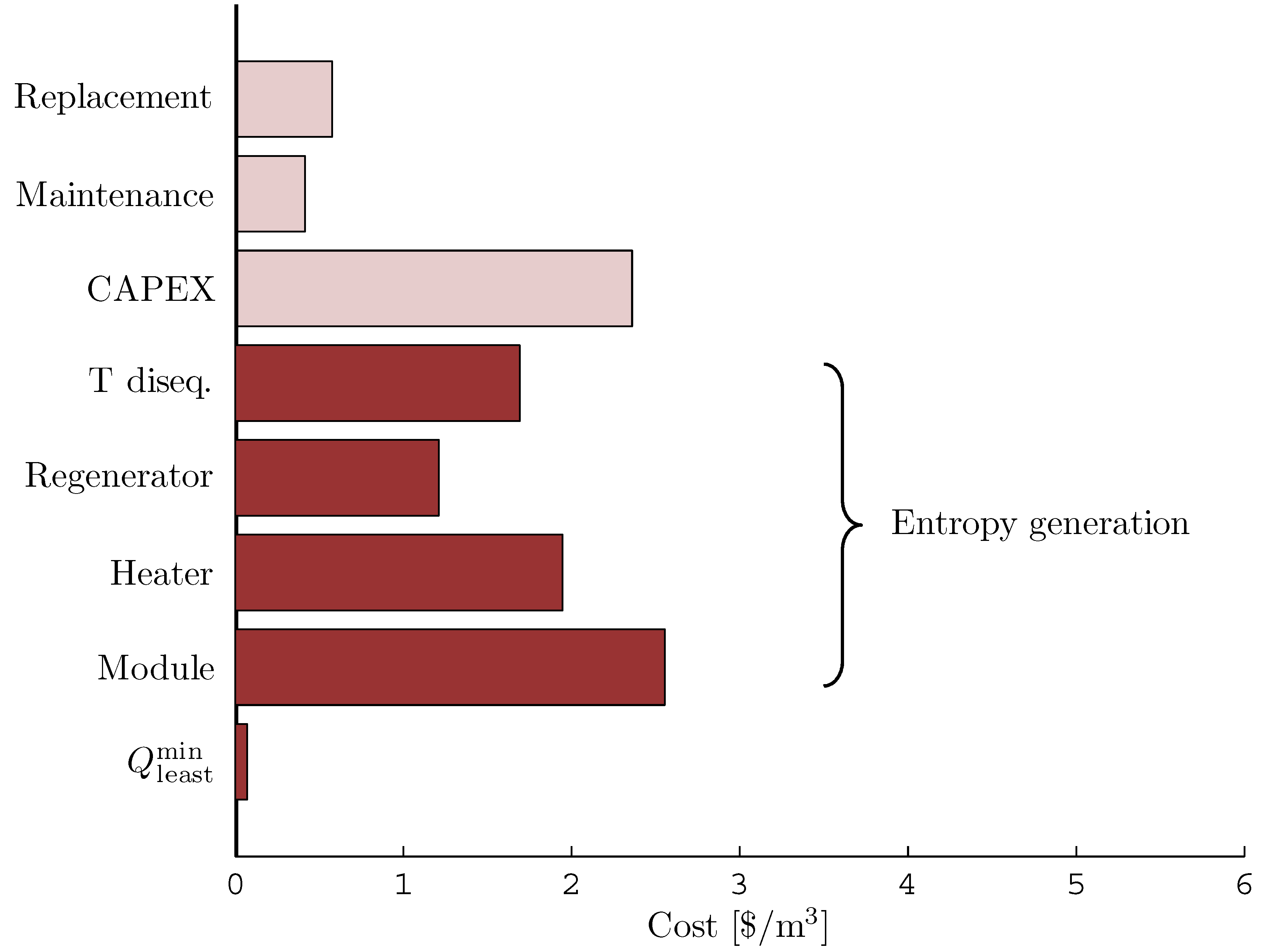
Since the cost of energy in the solar powered DCMD system is captured by the capital expense associated with building and installing the solar heaters, it is useful to separate that cost into its component parts. Namely, it can be split into the cost of the minimum least heat of separation and all of the entropy generation in the various components in the system and due to chemical and thermal disequilibrium of the discharged streams. The solar heater costs are split and compared to all the other costs in
Figure 9. It is clear that the costs associated with entropy generation in each component is of the same order of magnitude as the entire capital expense of the rest of the DCMD system. In particular, losses in the module are the single greatest source of cost for this system.
Figure 9.
Breakdown of costs associated with the production of water using direct contact membrane distillation with the cost of entropy generation expanded.
Figure 9.
Breakdown of costs associated with the production of water using direct contact membrane distillation with the cost of entropy generation expanded.
From this example, it is evident that freely available energy, such as solar power, is not truly free. The capital expense required to harvest the solar thermal energy is significant and, in some cases, can be the majority of a system cost.


