2. Irreversible Process
The basic postulate of the thermodynamics of irreversible processes refers to the entropy generation. As a result of the irreversible process proceeding in the element of volume
dV entropy generation is obtained with the rate of
σSdV.
σS ≥ 0, which is always a non-negative entropy generation rate (in unit volume and unit time), which equals zero only in equilibrium. The change of entropy in the given element
dV in the time period
dt is, however, the result of not only the entropy generation in the element itself, but it is also caused by an exchange of heat energy with its environment. Thus, it could be written as:
where
ds is the difference of entropy density,
T is the temperature and
dq is the difference of heat density, which is exchanged by the element
dV with its environment. Since there is always
σS ≥ 0, therefore:
Equality in relation
Equation (2) refers to reversible processes and non-equality to irreversible processes. In a system being in non-equilibrium conditions, gradients of intense state parameters (gradients of temperature and electrochemical potentials) occur. In semiconductors, relation
Equation (2) may be referred to as the selected kinds of charge carriers, which are treated as a system. We can distinguish, for instance, between electrons in a conduction band and holes in a valence band, ionized impurities,
etc. For the
i-type particles, relation
Equation (2) reads as:
The steady state is the goal of our considerations. In classical irreversible thermodynamics [
6–
9], it is presumed that small elements of a non-equilibrium system are in a state of local equilibrium, and equations of equilibrium thermodynamics hold well for such sub-system. This postulate is known as a local thermodynamic equilibrium.
Thus, considering the state of a small sub-volume
dV of the semiconductor heterostructure, one can apply Gibbs relation to express the differential of heat density
dqi of
i-type particles by the differential of density of their energy
dui, as well as the differential of particle density
dni. Then, inequality
Equation (2a) assumes the relation as:
where Φ
i is the electrochemical potential of
i-type particles (for example, electrons in a conduction band). In a steady state, both intense and extensive state parameters are stable in an arbitrarily chosen element of the volume
dV. Due to relation
Equation (3), the function:
which is determined in
dV should achieve maximum values in a steady state.
In a steady state, a source of entropy generates an entropy in each cell of space with a possible low rate. This is in accordance with Prigogine principle [
10,
11]. If we denote the efficiency of the entropy source (in J K
−1 cm
−3) for
i-kind particles as
, then in steady-state conditions:
The steady state being a non-equilibrium state is caused by stationary gradients of state intensive parameters (temperature and electrochemical potentials, usually called quasi-Fermi energies), which cause flows of energy and electric carriers. However, these flows take place in a very complex and complicated way, being the result of a huge number of single acts of an electron and phonon scattering in a dissipative process. The integration of relation
Equation (3) over all of the volume of the semiconductor structure leads to a relation of:
Let us denote as
Mi the following integral:
Thus, the right side of
Equation (6) is the differential
dMi of the function
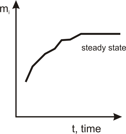
Mi. Since
dMi is always positive during the irreversible process, then, in the steady state,
Mi being of stable quantity achieves its maximum value. This value is stable as long as the steady state lasts (see
Figure 1).
Thus, in a steady state, the condition for the maximum of the following functional can be formulated as:
The state of intense parameters contained in functional
Equation (8) are space-dependent quantities; however, they do not change in time. Using the expressions for electron and hole energy, as well as for their entropy (
Equations (46)–(
49)), the function for the electron and holes can be derived as below:
and:
respectively. Here,
is the distribution function for electrons in a conduction band and
is the distribution function for electrons in a valence band.
Functional
Equation (8) for the electron and holes achieves the maximum if:
and:
respectively.
Equations (11) and (
12) are Euler–Lagrange (E-L) equations, and their solution are the functions:
It is apparent that the above functions cannot be the correct distribution functions by observing that they are even in the wave vector (kinetic energies
and
are square functions of
), and therefore, it can be predicted that current can never flow. Nevertheless, these are not unreasonable results considering that average carrier velocities are frequently small. If we measure the spread in velocities by the velocity at which
drops to
of its peak, we find a spread of about 10
7 cm s
−1 for a semiconductor with
m* ≈
m0 [
12]. Since average velocities are often much smaller than this, an assumption that the average velocity equals zero may be not as bad as it seems. However, we will try to find more correct expressions for the distribution functions.
3. Gyarmati’s Variational Principle of Dissipative Processes
Non-equilibrium processes arise either due to the action of thermodynamic forces, which prevent the system from reaching the equilibrium state, or due to the process of internal phenomena, resulting from certain types of relaxation processes [
13]. In the 1960s, Gyarmati proposed a variational principle, which describes the evolution of irreversible processes in space and time [
14,
15]. Gyarmati’s principle is based on the fact that the generalization of dissipation functions, which were introduced by Reyleigh and Onsager for special cases, always exist locally in continua [
16–
22]. In linear theory, these functions are defined as:
and:
The
Rik coefficients are the components of the inverse of the
Lik coefficient; hence, the existence of dissipation potentials is connected to the existence of the Onsager reciprocal relations. The current
Ji is conjugated to the force
Xi in the entropy production density
σS. σS being the entropy production per unit volume and unit time is a bilinear function of the independent currents
Ji and the conjugate dissipative forces
Xi, that is:
According to the Onsager’s linear theory of irreversible processes, the currents Ji and the dissipative forces
Xi are given by the following general constitutive laws [
20,
21]:
The most general form of Gyarmati’s principle is given by:
or:
Some weighted potentials Ψ
G and Φ
G can be defined, as well. They show all of the essential properties of Ψ and Φ, but correspond to the weighted entropy production
GσS [
23–
25] (here,
G is an arbitrary, always positive state function):
In some cases, in steady-state conditions, especially for strictly linear problems, there are two partial forms that are also valid [
25]:
and:
The first of these is called force, and the second is called flux representation. Both representations were applied to the solution of several practical problems (see the references cited in the paper of Verhas [
25]).
We will apply
Equation (23) for electrons and holes. The thermodynamic forces for electrons (see relation
Equation (72)) are recognized as:
and:
where:
4. Postulate of the Variational Principle for the Semiconductor Heterostructure in Steady-State Conditions
As was shown in Section 2, functional
Equation (8) is not sufficient to obtain the proper expression for a non-equilibrium distribution function for electrons in CB and VB. To achieve this goal, we postulate applying a new variational principle obtained through a connection of functional
Equation (8) with Gyarmati’s principle expressed by relation
Equation (23). In order to join them, we form the weighted potential Ψ
G by multiplying equation
Equation (23) by the mean relaxation time
. This proposed principle (for CB electrons) reads as:
Why should the acceptance
as the multiplier be a good choice? First, Gyarmati’s principle remains valid if it is multiplied by any non-negative state function and the average relaxation time is a non-negative state function. Second, it is a characteristic time during which electron scattering takes place by collisions. This time determines band electron mobility and their drift velocity. We show further that the postulate will allow us to determine a non-equilibrium distribution function, which for small gradients of intensive parameters is identical to the function resulting from the BKEsolution, which will confirm the postulated validity.
By comparing the coefficient expression
Equations (27)–(
29), we note that the coefficient
L22 is orders of magnitude less than the other three coefficients. Thus, in equation
Equation (26), we can skip the last component. Now, using
Equation (68) and using relations
Equations (9), (
25)–(
29), we can present the function λ
e in the form of:
Equation (34) for holes takes the form of:
Proceeding as with electrons, λ
h will take the form of:
4.1. The Non-Equilibrium Distribution Function for Electrons
Functional
Equation (34) achieves maximum value if the function λ
e meets the E-L equation, which means:
4.2. The Non-Equilibrium Distribution Function for Holes
Functional
Equation (37) achieves maximum value, if the E-L equation reads as:
While the distribution function of holes
fh will take the form of:
5. Verification of the Obtained Results
Here, we verify the obtained relation
Equations (40) and (
43) by comparing them with suitable results obtained by other authors using another method of analysis. The agreement of the results would be the confirmation that the postulated variational principles (relations
Equations (34) and (
37)) are suitable for analyzing the steady-state conditions in semiconductor heterostructures. Let us begin our considerations for the function
. We compare expression
Equation (40) with Expression (5.1) obtained by Marshak and van Vliet [
2] by a solution of the KBE under the assumption that the values of ∇Φ
n and
∇Te are low. We decompose relation
Equation (40) into the Taylor series around Φ
n and
Te under the assumption that ∇Φ
n and ∇
Te are of low values. As a result, we obtain the relation of:
It is easy to notice that expression
Equation (44) is the same as Expression (5.1) in the paper of Marshak and van Vliet [
2].
Similarly, by decomposing the function
fh around Φ
p and
Th under the assumption that
∇Φ
p and
∇Th are of small values and by confining ourselves to the first order words, we are going to obtain the following:
Expression
Equation (45) can be obtained similarly as what was done by Marshak and van Vliet [
2] by solving the BKE under the assumption that the gradients ∇Φ
p and ∇
Th are low. Thus, expression
Equations (44) and (
45) obtained in this paper are in agreement with the results obtained by solving the BKE in the special case. This confirms that the forms of functionals
Equations (34) and (
37) are proper and can be used to analyze semiconductor heterostructures in steady-state conditions
Expression
Equations (40) and (
43) are more general than the expressions for non-equilibrium distribution functions, obtained by solving the BKE. What is more, non-equilibrium distribution functions have the form of the Fermi–Dirac distribution function (with four additional components). The physical interpretation of these components is relatively simple. We explain it for
. The physical interpretation of suitable components in
fh is analogous to those in
.
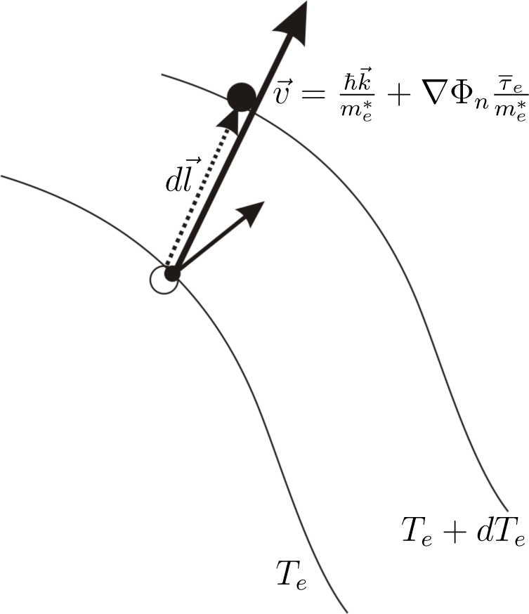
The expression
is equal to
dTe, the change of the electron s temperature in the time period equal to the mean relaxation time
(
Figure 2).
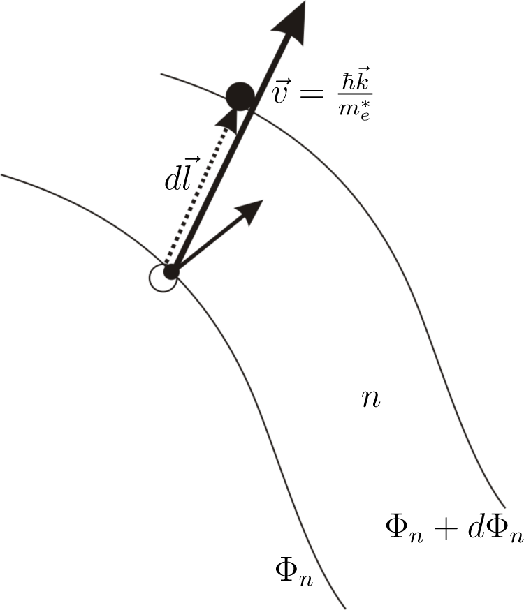
The expression
is recognized (
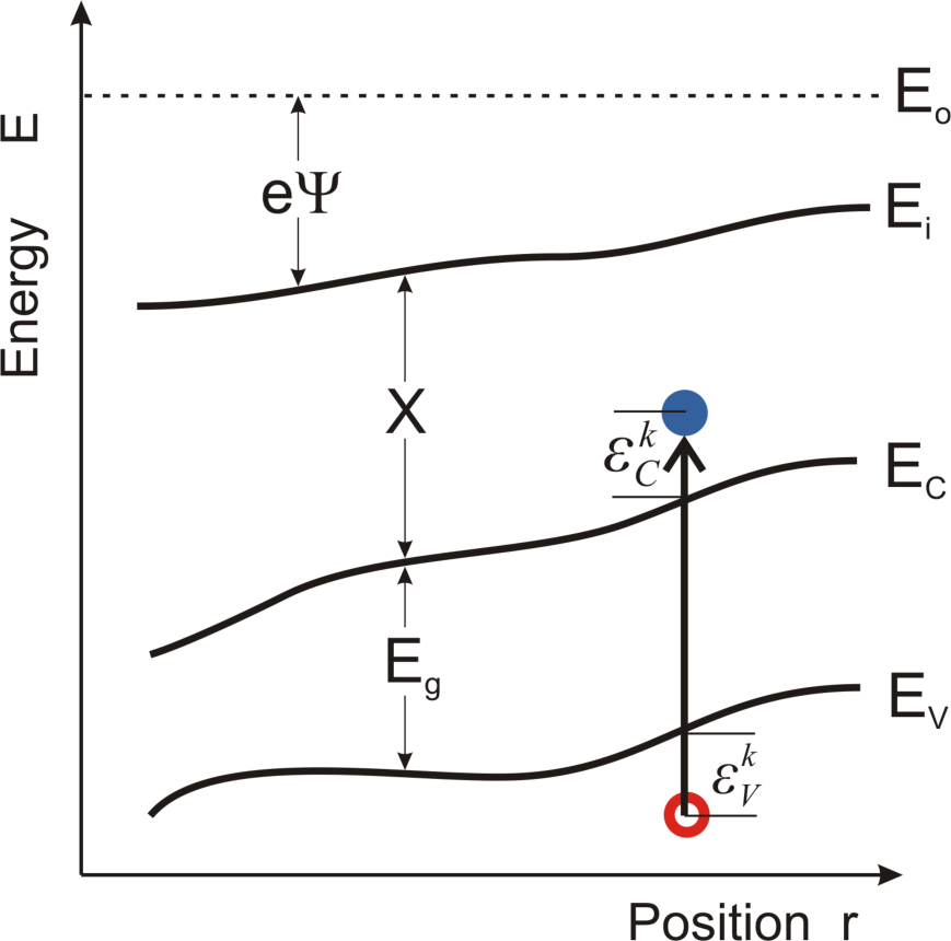
Figure 3) as a change of electron kinetic energy caused by the movement of the electron in the region where the gradient of quasi-Fermi energy occurs. The sign of this change depends on the direction of the electron velocity The expression
is found as an increase of electron energy caused by the force −∇Φ
n working on the distance
.
6. The Calculation Method and Its Exemplary Results
We discuss here the calculation method consisting of calculating the electron and hole distribution function, as well as presenting the exemplary results of the calculations for electrons (relation
Equation (40)). The calculations will involve ternary semiconductor compounds of mercury cadmium telluride (MCT) (Cd
xHg
1–xTe) with two chosen values of
x, a mole fraction of CdTe (
x = 0.165 and
x = 0.3), a concentration of donors
ND = 10
15 cm
−3 and acceptors
Na = 10
13 cm
−3. Data on the physical parameters of the material can be found, for example, in the book edited by Capper [
26]. While conducting the numerical modeling of devices, we are not able to calculate non-equilibrium distribution functions at the heterostructure selected points directly using only relation
Equations (40) and (
43). The calculations must be conducted by iterative methods, because
Equations (40) and (
43) are highly non-linear. In turn, these values are dependent on external forces maintaining a steady state and on a distribution function. First, our calculations begin for a thermal equilibrium state by solving the Poisson equation with iterative methods for given spatial distributions of a molar composition and doping. This allows the determination of the spatial distribution of electric potential, as well as the electron, holes and ionized dopant concentrations. In order to determine these concentrations, the Fermi–Dirac functions applicable to the thermal equilibrium state are used. The accurate description of this method is in the paper of Jóźwikowska [
27].
Next, by changing the boundary conditions on electrical contacts due to the value of the applied voltage, we solve the system of four or six transport equations with iterative methods. We gradually increase the voltage until it reaches a desired value. Subsequent changes to the voltage value are the condition for the convergence and stability of the iterative method used. In the first iterative step for the initial voltage, we make calculations by using the non-equilibrium distribution functions in the form of the Fermi–Dirac function for thermal equilibrium. In these functions, the Fermi level is replaced with quasi-Fermi levels, and we take into account that the electron and holes own a thermodynamic temperature, which can be different from the lattice temperature. For electrons in the conduction band and valence band, those are
Equations (13) and (
14), respectively. In subsequent iterations, we already use distribution functions in the form of
Equations (40) and (
43). Using these, we calculate both the carrier concentration, as well as the average relaxation time defined by
Equation (71). Counting the relaxation time in MCT, we take into account two mechanisms of scattering: ionized impurity scattering and polarized optical phonon scattering [
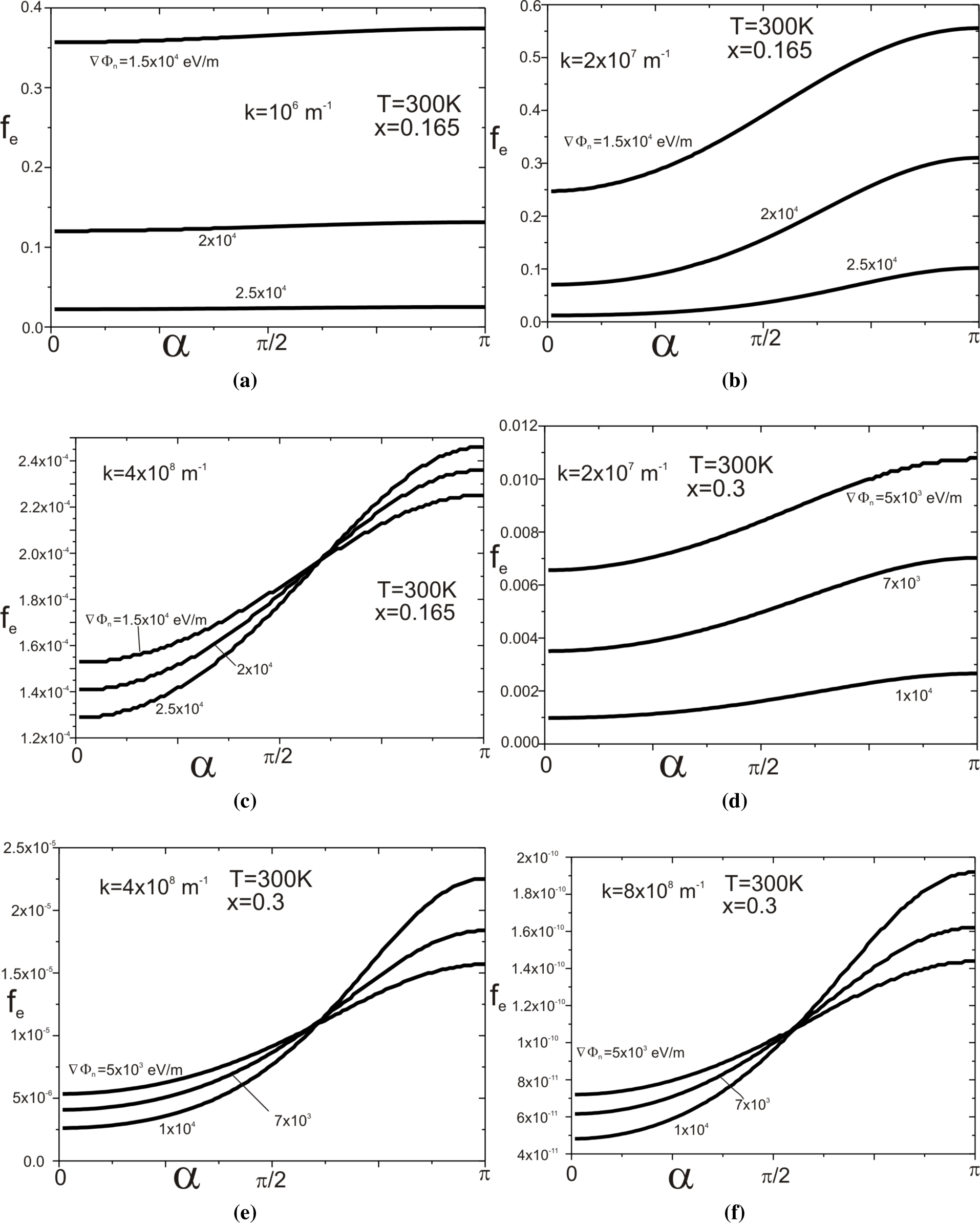
13]. Due to the fact that the effective mass of electrons in a HgCdTe narrow gap is more than an order of magnitude less than the effective mass of holes, effects related to the gradient influence of intensive parameters are in the case of the electron distribution function much stronger than for holes. Therefore, the exemplary calculation results are shown for the non-equilibrium distribution function for electrons, as they are the most spectacular. As we analyzed the semiconductor instruments, temperature gradients are usually very small, and their impact on the non-equilibrium distribution function is incomparably smaller than the impact of the quasi-Fermi level gradients. In the cases presented here, the influence of a temperature gradient on the function
is negligible.
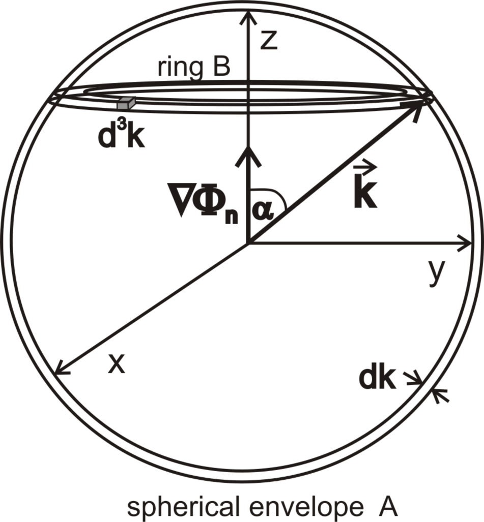
Figure 4a–
4f presents the dependence of the function on the angle, which the wave vector
creates with the vector ∇Φ
n for selected modules of the vector
and the selected gradients ∇Φ
n (see
Figure 5).
Figure 4a–
4c relates to the structure of the molar composition
x = 0.165 and the temperature
T = 300 K, and
Figure 4d–
4f relates to the structure with parameters
x = 0.3 and
T = 300 K.
Now, it is evident that distribution functions determined by relation
Equation (40) are not even in the wave vector, in contrast to those determined by relation
Equation (13).
determines it. When the dot product
is positive, it increases the potential energy of a moving electron at the expense of kinetic energy. Reducing the kinetic energy leads to increasing the value of
. When the movement direction is the opposite, then the electron potential energy decreases, and its kinetic energy increases. Hence, the increase in value of the function
is with the increase at the angle
α. The impact of the component
on the function
becomes increased with both the increase of module
vector and with the gradient value ∇Φ
n, which is well illustrated by
Figure 4.
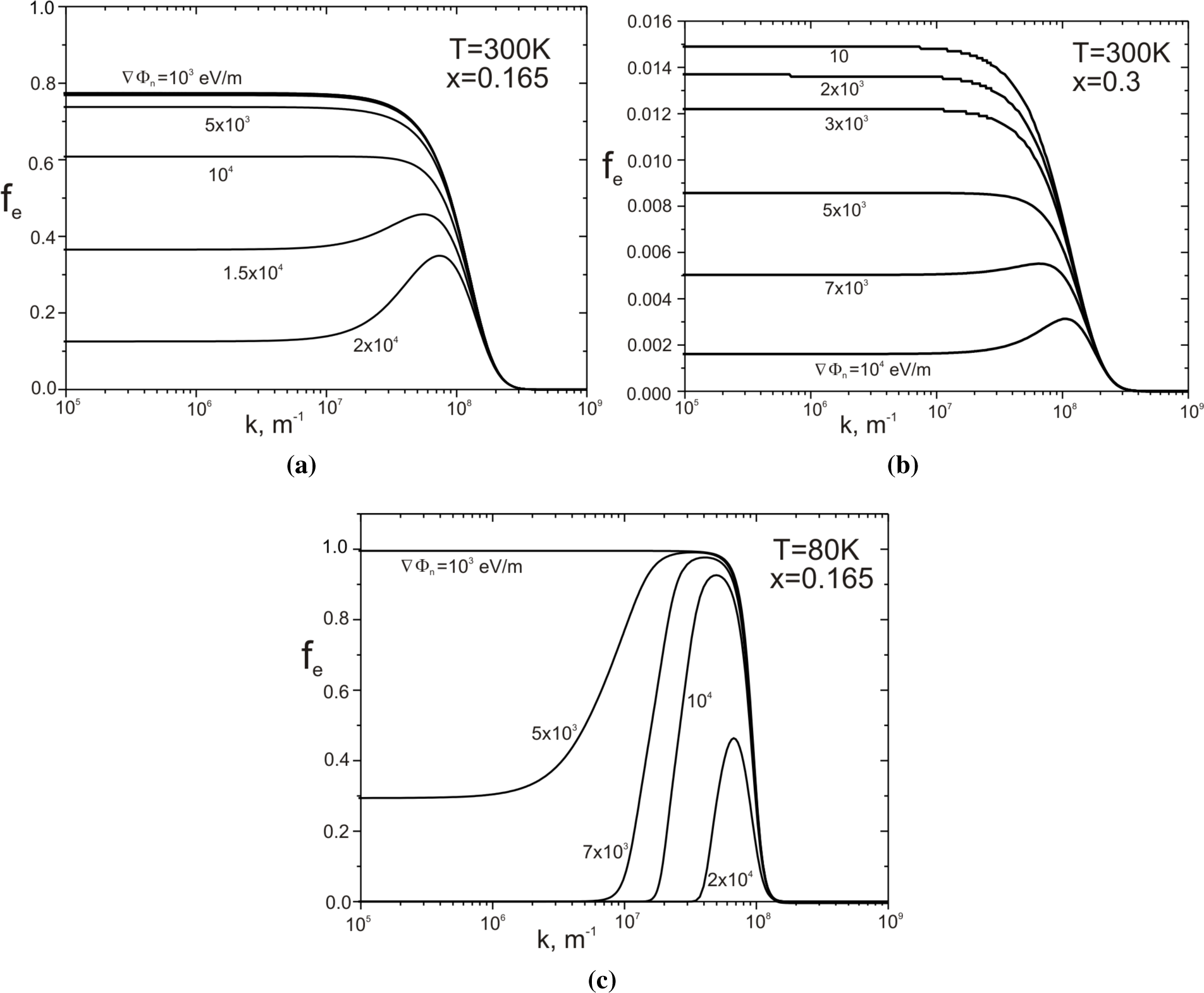
Figure 6 presents the dependence of
on the wave vector module
for the selected gradient values ∇Φ
n (numbers with curves). The presented values of the function
are mean values for cells that form the spherical Envelope A (see
Figure 5).
Figure 6a describes the structure with the parameters of
x = 0.165,
T = 300 K;
Figure 6b, x = 0.3,
T = 300 K; and
Figure 6c, x = 0.165,
T = 80 K. For
k < 10
7 m
−1,
weakly depends on
k, but rapidly disappears with increasing
k for
k > 10
8 m
−1. The reason for this failure is the kinetic energy
increase, which is a quadratic function of the wave vector
. Increasing the kinetic energy component
is the reason for the observed decrease in the value of
with the increasing values of ∇Φ
n. However, the increase of the value of ∇Φ
n increases the role of the component
, which depending on the sign of the scalar product
, can cause either an increase or decrease in the value of
. This component of the overall balance will increase the average value of the function
, which is noticeable for sufficiently large values of the gradient ∇Φ
n. This is particularly shown in
Figure 6c, where the influence of this component in the range of values 10
7 m
−1 <
k < 10
8 m
−1 seems to be dominant. This is achieved by the addition of average relaxation time, which grows with a decreasing temperature. Calculated by us,
, for the material
x = 0.165 at
T = 300 K is 4.17 × 10
−12 s and at
T = 80 K is 7.3 × 10
−12 s.
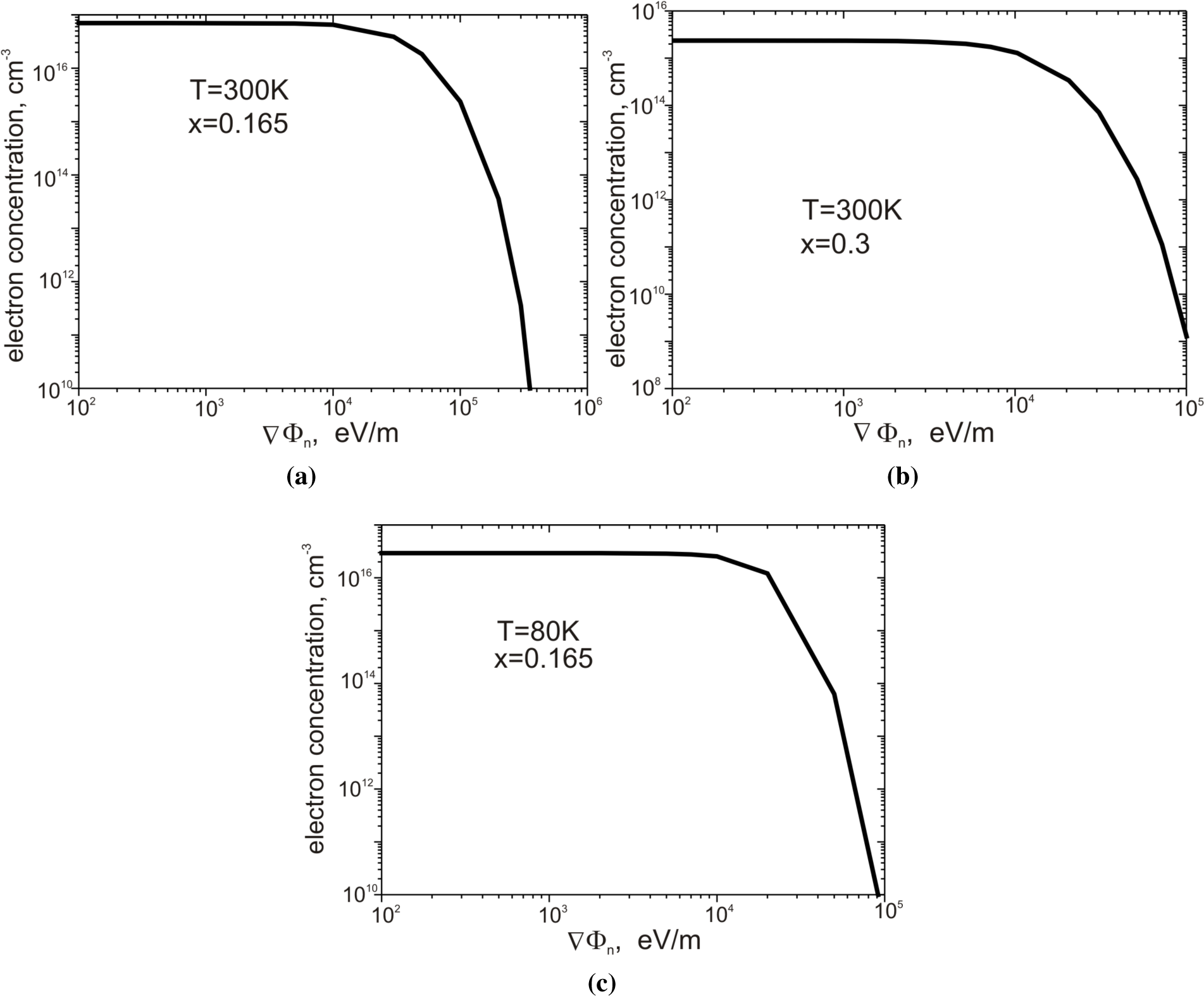
Figure 7a–
7c presents the dependence of electron concentration on the value of VΦ
n.
Figure 7a shows the structure with parameters
x = 0.165,
T = 300 K;
Figure 7b,
x = 0.3,
T = 300 K; and
Figure 7c,
x = 0.165,
T = 80 K. In all three cases, the electron concentration remains almost constant for gradients ∇Φ
n < 10
4 eV m
−1. The increase of the gradient ∇Φ
n up to the value of 10
5 eV m
−1 results in a reduction of the concentration in all cases by several orders of magnitude. The obtained values of electron concentration are in good agreement with the experimental data presented by Capper [
26].


