2.1. Image Preprocessing
Image alignment is the first step necessary for an efficient automatic computerised classification procedure of X-ray images, since many patients with fractures of the ulna and radius bones are not capable of aligning their hands properly in an X-ray machine, resulting in angled images (as shown in
Figure 1a). Although image alignment is not a problem for visual inspection done by radiologists, it is important in the proposed image segmentation algorithm. Thus, the image alignment stage of the proposed algorithm consists of the following steps:
Enlarging the border of the input X-ray image;
Transforming the grayscale image into a black and white image;
Calculating the vector describing the orientation of the image by utilising the PCA method; and
Adjusting the image, so that the vector of the image orientation is aligned with the vertical axis of the background canvas.
In post-processing, clinical X-ray images of children’s extremities should not be electronically cropped beyond the borders of the physical radiation-beam collimation [
15], as shown in
Figure 1a. The extraction of the resulting angled box coordinates can be improved by enhancing the border between the box and the image frame, which is achieved by inserting a padding of 10 black pixels to the image frame, as shown in
Figure 1b. To enhance our region of interest, the image content was transformed to black & white, based on the intensities of the image pixels
:
The above-mentioned thresholding resulted in the image shown in
Figure 1c. It can be seen that the resulting image of this phase contains several artefacts (namely, black regions inside the white box). These artefacts are removed using a morphological closing operation, with a kernel shaped by an all-ones matrix (with dimensions
) [
16]. This is a necessary pre-processing step, preceding the box vector calculation, due to its sensitivity to unwanted artefacts.
The next step consists of calculating the angle defining the direction of the box, which represents the region of interest. Utilising traditional methods (such as a Canny filter or Sobel operator) to detect the edges of the box results in edges which can be transformed into vectors [
17]. Next, it is necessary to define the centre of the box and the angle between the vector and the horizontal axis of the image. However, instead of white pixels being treated as a part of the box, they are treated as data points. In addition, note that every data-set has defining features (such as standard deviation, variance, mean value, and so on). Here, we employ PCA as a statistical procedure which uses an orthogonal transformation of the original space to convert a set of observations of possibly correlated variables (entities, each of which takes on different numerical values) into a set of values of linearly uncorrelated variables, called principal components [
18]. The first principal component has the largest possible variance (to preserve as much variability in the data as possible). In our case, the first principal component is the vector having the same direction as the white box, as shown in
Figure 1d (the angle between the vector and the horizontal axis is denoted by
). Once the angle of rotation is calculated, the whole image is rotated around its centre by
.
Next, the missing pixels caused by rotation are interpolated, using Lanczos interpolation over an
neighbourhood [
19]. The described procedure, with some fine tuning, could be used for aligning any X-ray image whose content is inside of the box.
Figure 1e displays an example of an aligned image. The described pre-processing ensures the rotation-invariant property of the proposed computer-aided automatic solution for X-ray image segmentation and fracture detection.
2.2. Local Entropy-Based Tissue Removal
A key problem in bone segmentation is the differentiation of tissue from actual bones. Therefore, to solve this problem, we introduce a modified method based on the Shannon entropy (also known as information entropy). The Shannon entropy, previously shown to perform well on a similar problem [
20], represents an average rate at which information, usually measured in bits, is produced by a stochastic data source:
However, this paper introduces a concept of local (short-term) Shannon entropy. Basically, the idea is to calculate the entropy inside of a sliding window (having dimensions ). Namely, the window slides through the picture with a stride of 1 pixel, and local entropy is calculated for each centre pixel, based on all other neighbouring pixels inside the window.
In the Equation (
2),
is the distribution of pixel intensities inside the window,
b is the logarithm base (often set to 2 for bits, as also used in the paper), and
is the size of the window (based on the extensive experimental research on training data,
n was set to 9). The local entropy of border and near-border pixels was calculated by mirroring nearby pixels to fill the missing pixel intensities inside the sliding window. It is important to note that this mirroring is applicable for arm X-rays, because there is usually no tissue or any other useful information near image borders.
The resulting local entropy representation of the image can be treated as a measurement of bone presence. Namely, when pixels inside the window have a similar intensity, the entropy is low. On the other hand, when the bone is captured inside the window with the surrounding tissue, the entropy is high, due to pixel intensity diversity. Next, in order to emphasise this difference, we propose multiplying the local entropy by the standard deviation of the pixels inside the window:
The resulting images are given in
Figure 2.
As shown in the entropy figures, the bone edges remain clearly visible, with only a small amount of tissue and noise left in their vicinity. In order to additionally emphasise the contours of the bones and to obtain a black and white image (with white pixels representing just bone contours), we have tested several edge-detection algorithms and proposed a new one, which outperformed all of them for the tested data-set [
21,
22]. In particular, the tested algorithms are:
Canny filter;
Sobel operator (x and y axis);
Laplacian edge detector; and
The proposed algorithm for line-edge detection.
The proposed algorithm searches for peaks in pixel intensities for each row of the local entropy image from the previous step of the method (entropy image), where high pixel intensities represent bones. The goal of the proposed algorithm is to preserve high value pixels and to remove low value pixels (representing noise and tissues). In order to do so, the proposed algorithm consists of several steps detailed in sequence (the algorithm is explained for one image row, and the same procedure is repeated for every row of the entropy image):
The first step is image normalisation: The image is smoothed by subtracting the mean of all pixel intensities from the original pixel intensity (with negative pixel values obtained by subtraction, being set to 0). This step results in improving the difference between bone and tissue. It also partly removes blurring around the bone, as shown in
Figure 3a (the red line in the image denotes a random row chosen for demonstration of this method’s step).
The next step examines a distribution of pixel intensities along each row (as shown in
Figure 3b, for the red line row denoted in
Figure 3a). All large peaks in the graph represent bones in the image. Hence, the next step of the algorithm is to extract the peaks.
Peak extraction can be performed by finding the local maxima in the graph values. The local maxima in
Figure 3c are denoted by a red “x”. As can be seen, there are a significant number of false positive local maxima detected. Hence, local maxima filtering is required as the next step. Note, also, that a simple thresholding of high value pixel intensities (unlike the low value pixels) is not applicable, since bones are usually represented by several connected pixels in a row, having similar (high) intensities. Namely, thresholding would, in many cases, eliminate both bone contours and false positives.
Thus, in order to eliminate false positive peaks, neighbouring pixels having the same or similar intensities, which are marked as the peaks, are combined into one peak. Thus, instead of a “region” of local maxima, only one representative pixel of the region is kept. The representative pixel is placed at the mean coordinate of the pixel region belonging to the representative pixel.
In addition, zero-valued pixels are removed from bone contours by applying hard thresholding (threshold value is set based on the intensities of pixels larger than 0). Experimental tests using a grid-search algorithm show that a threshold of 20% performs better than mean, median, and quartile thresholds, suppressing most of the noise and preserving all of the peaks which represent bones (as shown in
Figure 3d).
The final result of the proposed bone extraction procedure for the whole image (all rows of the image) is given in
Figure 3e, where the white pixels represent bones.
The proposed bone extraction algorithm is also presented in a diagram, shown in
Figure 4.
In order to compare the performance of the proposed method to other segmentation and contour-detection algorithms, the noise left after image segmentation (tissue removal) was measured using the global entropy measure (calculated as the sum of image entropy and segmentation entropy).
Namely, the image entropy measures the amount of information left in the image after segmentation (
2).
On the other hand, segmentation entropy may be used as a measure for noise artefacts and small-noise fragments left in the image (since a single white pixel or small region of white pixels does not represent a bone). In particular, a bone is represented by a relatively long line of pixels. Hence, measuring artefacts may be reduced to measuring non-bone regions of white pixels done by the segmentation entropy (proposed by J. Hao [
23]). The segmentation entropy was defined as the sum of the image entropy
, subtracted from the entropy of
n windows (
), and divided by the image entropy
:
Finally, noise evaluation was obtained by combining the image entropy and the segmentation entropy (scaled by the number of windows):
All algorithms were first fine-tuned, in order to reach their best performances, on a training set consisting of 100 randomly chosen images from a data-set of 960 images, leaving 860 images as a test set. The hyperparameters for each algorithm, which resulted in its best performance, are as follows:
Canny filter: The lower and upper borders were set to , where is the standard deviation of pixels intensities and is the mean value of the pixels intensities of the input image;
Laplacian filter: The dimensions of the standard kernel for the Laplacian filter were set to ; and
Sobel filters: The dimensions of the kernel were set to .
The comparison of the proposed method to the Canny filter, Laplacian edge detector, and Sobel operator (both vertical and horizontal) for the test data-set is presented in
Table 1. As can be seen, the two methods that stood out among the tested methods are the Canny filter and the proposed method. The Canny filter was negligibly better than the proposed method in artefact detection—by
bits, in terms of the segmentation entropy. However, the proposed method outperformed the Canny filter by
bits, in terms of information preserved in the image after segmentation (image entropy). Namely, on the global scale, the Canny filter resulted in a larger number of false positives than the proposed method. When segmentation and image entropies were summed, the global entropy measure was obtained and the proposed method outperformed the Canny filter by
bits. In other words, the proposed method resulted in an image that preserved the highest number of bone pixels, and removed the highest number of tissue pixels.
2.3. Extracting the Region of Interest
The next step in the proposed method is extracting the region of interest (i.e., detecting its boundaries), which in our case contains ulna and radius bones. The bottom boundary is trivial to set (bottom of the image). However, finding the top boundary is based on detecting the correlation between the number of peaks in a row, and the place where ulna and radius bones end. As shown in
Figure 5a, there is a large jump in the number of peaks in a row related to the place where radius and ulna bones end (
Figure 5b). In order to narrow the search area for the peak with maximum value, the first
and the last
of the image is cropped out. In general, the ulna and radius bones do not end in the top or the bottom
of the real-life X-ray images (if so, the image is considered invalid). Hence, the end of ulna and radius connection is often found close to the image centre [
24].
The next step is to extract the highest peaks from the graph, shown in
Figure 5a. First, the local maxima regions were found (reduced to a single point/peak detection, as in Step 4). Next, only the peaks higher than 95% of the maximum peak are retained (resulting in just a few such peaks), as shown in
Figure 5a. Based on extensive experimental investigation, performed on the 100 images from a training set, it was shown that the far right peak in
Figure 5c properly localises the ends of the ulna and radius bones. Namely, the other lines usually represent parts of the wrist. The result of cropping, based on the cropping position detected in
Figure 5c, is shown in
Figure 6.
Finally, the image width is cropped by finding its left and right boundaries. Width cropping is based on the observation that, usually, peaks representing bones have the highest value. Because two bones are to be detected, four highest values are taken into account. The proposed method for finding the width of the region of interest is based on the average coordinates of four highest values of each row in the previously cropped image. In particular, this procedure can be divided into four steps:
Finding the coordinates of four highest peaks of each row in the image;
Sorting the coordinates from lowest to highest;
Finding the average coordinates values for sorted coordinates;
Extracting the lowest and highest coordinates which represent bone boundaries (bone boundaries are expanded by of the bone boundary area, in order to keep some additional area around the bones in the cropped image); and
Cropping the image with respect to the set boundary box.
The red marks in
Figure 7a denote the boundary box corners, with the final cropped image presented in
Figure 7b.
2.4. Bone Extraction
Following the detection of the region of interest, the next step is to create a black and white image of the bone contours. To extract bone contours, we propose a novel method, based on graph theory, utilising several observations specific for long-bone X-rays:
The bones are oriented along the vertical axis.
Bones start at the very bottom of the cropped image (where, in ideal noise-free images, only four starting points can be found).
With regard to the previous observation, for real-life noisy images, false positive lines may be detected, as well as blurred bones, which must be eliminated with an approximation of the actual bone contour.
In order to apply this bone extraction approach to other X-ray images (i.e., not containing long bones), similar regularities and rules should be noticed and implemented. Based on the above-mentioned observations, the proposed graph-based algorithm for bone detection consists of the following steps:
Root node selection;
Finding the next pixel that belongs to the bone;
Building a bone graph; and
False bone-pixel elimination.
2.4.1. Root Node Selection
Referring to the presumption that the bones are aligned along the vertical axis, here we introduce a bone detection procedure starting from the bottom of the image (knowing that the next bone pixel is to be found above it). Hence, the root node is to be found at the very bottom of the image. For this purpose, a black and white peak image is generated (shown in
Figure 8a for the input image presented in
Figure 8b), having white pixels where the intensities of the pixels are the highest.
In real-life scenarios, due to the noise (which is manifested as blurriness), the last line may have more than four white pixels representing the bones. Hence, in this step, all pixels found in the last line are taken as root nodes, and are forwarded to the next step of the algorithm (finding the next pixel that belongs to the bone). In the ideal case, only four pixels are detected as root nodes and, ideally, there are only four lines representing bones. Simulations performed on the training data set have shown that cases with four root notes are rare, and, therefore, image segmentation pre-processing is even more important.
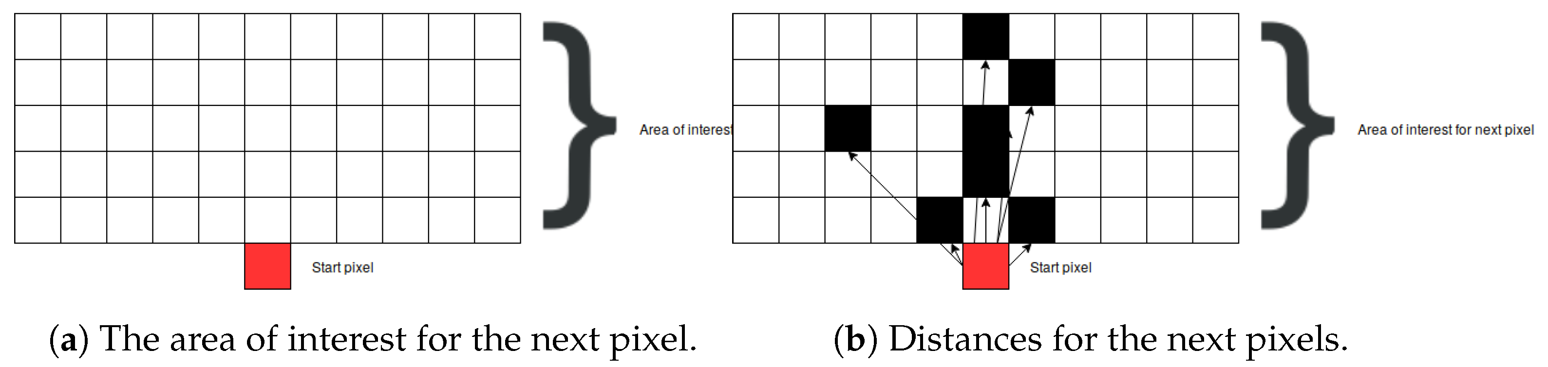
2.4.2. Finding the Next Pixel That Belongs to the Bone
Finding the next pixel from the respective root node is based on a graph-search algorithm. First, the area of interest, containing the next bone pixel, is defined. Knowing that the next bone pixel is to be found above and close to the current bone pixel root node (i.e., the first starting pixel at the far bottom of the image), the boundaries of the area of interest are set to 5 pixels above the current pixel and to 5 pixels to the left and the right hand side of the current pixel (as demonstrated in
Figure 9a). The current pixel is marked as a red square, and all other pixels in the area of interest are marked as black squares. Next, the Euclidian distance is calculated from the current pixel to all other pixels in the area of interest whose intensity is larger than 0:
where
and
are pixels.
After calculating all the distances, the pixel closest to the root pixel is returned. In the cases where there are multiple pixels having the same distance value (as shown in
Figure 9b), all of them are returned as a result and further processed by adding them to the graph.
2.4.3. Building a Bone Graph
The procedure for building a graph that represents the bone edges starts from the root pixel and searches for the next pixels (according to the previously-explained algorithm), which are added to the graph as children of the root pixel (children of the root node of the graph). For every child node, the process is repeated (i.e., the next pixels are detected and added as nodes in the graph). The procedure is repeated until the algorithm finds a node that does not have any children, and all nodes are expanded. The last node is the one having the smallest horizontal axis coordinate, while the first node is the one having the largest horizontal axis coordinate.
Finding the proper path from the first node to the last node is performed by calculating all of the paths and choosing only the ones whose length is more than the preset percentage of the image height. Namely, this preset percentage value is the hyperparameter dependent on the patient age (based on the experiments on the training set, it was set to
). The resulting image was shown in
Figure 10. Next, the last part of image preprocessing is to eliminate false bone contours.
2.4.4. False Bone-Pixel Elimination
The last problem in the proposed bone X-ray pre-processing pipeline is caused by blurry bones, which results in multiple lines for every bone contour. To solve this problem, a merging method, which combines multiple bone contours into one, has been proposed. It is important to notice that blurry bones, in general, cause several contours which are close to each other. For this purpose, we propose searching for additional contours in the vicinity of the initial one (i.e., inside a window of 15 pixels), which are then merged into one (on the row basis). Namely, for each row bone, pixels neighbouring the considered bone contour pixel (inside the widow width) are merged, and their mean pixel coordinate is set to represent the true pixel position. The described process is illustrated in
Figure 11, where two black lines are merged into the red line.
2.5. Fracture Detection
The final, and most important, step of the proposed method is the fracture detection procedure (especially for small, demanding fractures). The algorithm calculates the error between the ideal bone line, and the bone line extracted from the captured X-ray image using the method described above. The ideal bone line can be considered as a smooth high-polynomial curve and, hence, polynomial regression was used to obtain the ideal healthy (i.e., fracture-free) bone contour. For polynomial regression to work, the curvature at the top of the bone must be removed (since it produces too much noise). To remove this part of the curvature, an algorithm is proposed for seeking the highest peak in the curvature and cropping the bone line. The curvature is measured by a second degree polynomial in the top pixels of the bone line. Once the second degree polynomial is fitted to the top pixels, the peak of the polynomial is set as the cropping point.
Next, the difference between the previously-estimated healthy bone line and the bone line extracted from the X-ray image is calculated, in terms of the mean squared error. The corresponding pixels are pixels having the same horizontal axis coordinates (as shown in
Figure 12,
Figure 13,
Figure 14 and
Figure 15), representing four bone lines of the two bones. Namely, the red line in the figure represents bone pixel intensities, while the green line represents the contour approximation of the ideal healthy bone obtained by polynomial regression (a 3rd order polynomial, due to the shape of the bone).
Next, the fracture in the bone was detected by tracking the mean squared error between the polynomial approximation and the original bone contour. Based on the analysis performed on the training data set, and taking into the account the blurred bone imperfections and inaccuracies in contour pixel position estimation caused by bone merging, a tolerance of 3 pixels was implemented.
The final fracture detection and localisation results are shown in
Figure 12,
Figure 13,
Figure 14 and
Figure 15 (denoted by blue lines).
Figure 12 and
Figure 13 show two peaks which represent potential fractures. The critical fracture area is marked in the X-ray image by a red circle (at the centre of which is the coordinate of the highest peak, with radius being defined by the width of the area), as shown in
Figure 16.
As can be seen, the proposed method was shown to be efficient, not only in detecting the fractures in the images (flagging the images as either containing fractures or fracture-free), but also precisely localising the position and the size of the region with the fracture. This can be used to assist medical staff to consider only the images with fractures and to direct their attention to specific regions of interests containing demanding fractures.
In addition, one of the advantages of the proposed method is its possible application in labelling large data sets of medical images (with accurate specification of the fracture positions) to be used for training classification models based on neural networks and deep learning (supervised learning). This could enable an even more refined classification of fractures in the regions already detected by the method proposed in this paper. However, neural network-based classification is out of scope of this paper and is planned to be investigated in our future work.
In particular, the proposed hybrid method may be considered as a useful tool and an important step towards the replacement of tedious X-ray image labelling, done manually by medical experts, by the automated computerised method proposed in this paper.


