Flow through pipes and conjugate heat transfer find wide applications in industry. In the flow system, the hydrodynamic losses can be attributed to the frictional and local losses associated with the flow path changes. The hydrodynamic losses are irreversible and result in entropy generation in the flow system. Consequently, entropy generation gives insight into the amount of losses, which take places in the flow system. Considerable research studies were carried out to investigate the flow through pipes. A thermally developing laminar flow in pipes due conjugate heating was studies by Bilir [
1]. He observed that the Peclet number considerably influenced on heat transfer characteristics. The simultaneous wall and fluid axial conduction in laminar pipe-flow heat transfer were studied by Faghri and Sparrow [
2]. They showed that the Nusselt number exhibited fully developed values in the upstream region as well as in the downstream region (directly heated region). A low-temperature variational method was introduced by Gariban et al [
3] to calculate pressure drop and heat transfer for turbulent flow in ducts. The analysis led to development of Green’s function, which was useful for solving a variety of conjugate heat transfer problems. The transient conjugated heat transfer in developing laminar pipe flow was investigated by Al-Nimr and Hader [
4]. They showed that increasing the conductivity and the diffusivity ratios increased the thermal entrance length of the tube. The quasi-steady turbulence modeling of unsteady flows was studied by Mankabadi and Mobarak [
5]. They indicated that the rapid distribution theory provided the Reynolds stresses without use of the eddy-viscosity concept. The channel and the boundary layer flows were investigated by Chein [
6] introducing a low Reynolds-number turbulence model. He showed that the model proposed compared well with the measurements and yielded better predictions of the peak turbulent kinetic energy than the standard two-equation model. The behavior of friction and heat transfer coefficients of water flowing turbulently in a large circular pipe was investigated by Choi and Cho [
7]. They introduced a new turbulent heat transfer correlation for the prediction of the local Nusselt number. The heat transfer in the thermally developing region of a pulsating channel flow was studied by Young et al [
8]. They indicated that dominant contribution to the change in Nusselt number stem from the additional axial transient effect. The numerical simulation of transitional flow and heat transfer in a smooth pipe were studied by Huiren and Songling [
9]. They showed that in the fully developed region flow and heat transfer were not affected by inlet temperature and the agreement between the results and data for the friction coefficient was good. Al- Zaharnah et al [
10] studied the conjugate heat transfer in fully developed laminar pipe flow and thermally induced stresses. They showed that thermal stresses amplified as heat flow on the wall increased. Al-Zaharnah et al [
11] investigated pulsating flow in circular pipes. They indicated that the effect of pulse frequency on the temperature distribution became insignificant as the Reynolds number was lowered.
Thermodynamic irreversibility occurs in the flow system due to fluid friction and heat transfer. The amount of thermodynamic irreversibility gives insight into the losses associated within the thermal system. Moreover, entropy production rate provides information on the amount of thermodynamic irreversibility in the system. Consequently, prediction of entropy generation due to different flow conditions enables to determine the flow system with minimized losses. Considerable research work was carried out to investigate the importance of entropy generation in the thermal systems [
12,
13,
14,
15]. Entropy generation and minimization were investigated extensively by Bejan [
16]. He showed the fundamental importance of the entropy minimization for efficient processing. The second law analysis of combined heat and mass transfer in internal and external flows was considered by Carrington and Sun [
17]. They introduced the entropy correlation, which could be used for internal and external flows. Heat transfer and entropy generation for a transparent gas flow were considered by Gbadebo et al [
18]. They indicated that the maximum volumetric entropy generation became independent of tube length for high heat transfer coefficients. The local entropy generation due to impinging jet was investigated by Shuja et al [
19]. They showed that the minimum entropy generation concept alone might not be used to evaluate the various turbulence models, in which case, the experimental measurements were accompanied with the results of entropy analysis.
The entropy generation in the flow and heat transferring systems, gives the amount of thermodynamic irreversibility associated with the thermal system. Consequently, investigations into entropy generation in the flow and heat transferring system is fruitful. In the present study, the numerical investigation of turbulent flow in a pipe with external heating situation is considered. The flow and temperature fields are computed using a numerical method employing a volume approach. Entropy generation due to fluid flow and heat transfer is predicted. In the simulations, temperature dependent viscosity is accommodated. In order to account for the turbulence, k-ε turbulence model is accommodated.
Mathematical Modeling and Numerical Solution
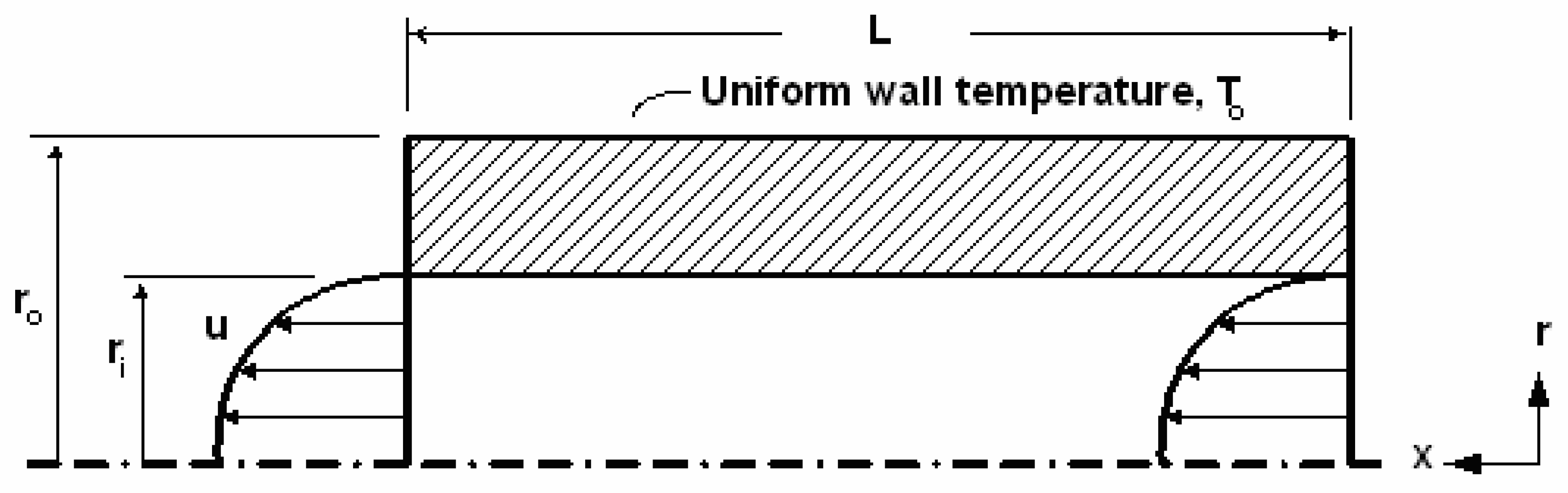
The flow situation in the present study is involved with an incompressible flow through a pipe, which is externally heated at different temperatures. The pipe is shown schematically in
Figure 1. The flow field is assumed to be axisymmetric and a uniform outer wall temperature is assumed along the pipe length.
The equations governing the flow field are simplified after the consideration of Boussinesque approximations, in which case k-ε turbulence model can be used to account for the turbulence characteristics. In cylindrical polar coordinates the conservation equations are written as:
Continuity:
Momentum:
Energy:
where Pr and Pr
t are laminar and turbulent Prandtl numbers respectively.
In order to determine the turbulent viscosity and the Prandtl number, the k-ε turbulence model is used. The constitutive equations for the turbulent viscosity are as follows:
where k and ε are the turbulent kinetic energy generation and the dissipation variables respectively. The transport equation for k is:
Where
The transport equation for ε is:
The generation of turbulence kinetic energy, ε and its dissipation at the inner wall of the pipe (r = r
i) is zero. The Prandtl numbers in transport equations of kinetic energy generation and dissipation are Pr
k and Pr
ε, respectively. The Prandtl number varies with Reynolds number [
20]. The values in
Table 1 are employed during the simulations, since each simulation is carried out for a fixed Reynolds number.
In order to minimize computer storage and run times, the dependent variables at the walls were linked to those at the first grid from the wall by equations, which are consistent with the logarithmic law of the wall. Consequently, the resultant velocity parallel to the wall in question and at a distance y
1 (where y
+≤30) from it corresponding to the first grid node was assumed to be represented by the law of the wall equations [
21], i.e.:
where, κ is a universal Von-Karman constant and e is a universal turbulence parameters and their values are κ = 0.417 and e = 9.37, from which the wall shear stresses were obtained in solving the momentum equations. The constants used in the transport equations are [
21]:
A radial step length of approximately two viscous sub-layer thickness (y
+ = 5), where y
+ = y [(τ
w/ρ)
1/2/(μ/ρ)] is employed. In the axial and radial directions, the grid contains 64 × 300 nodes in the fluid region and 64 × 100 nodes in the solid region, employed to obtain the grid independent solution. The grid nodes are distributed to give high concentration grid lines near the wall provided that the wall adjacent nodes are positioned at y
+ ≈ 5. The grid independency tests were carried out by using the different grid nodes and the grid distribution tests were also conducted and based on the findings, the grids giving optimum solution is ensured as consistent with the early work [
20]. To validate the numerical predictions, the experimental results presented in the literature [
20] are considered. In this case, the simulation conditions were set with similar conditions. The Nusselt number (Nu) predicted from the present study is 77.5 and that presented in the previous study [
20] is 80. The small discrepancy may be due to slightly over predicting the turbulent kinetic energy generation by the turbulent model (k-ε model) introduced in the present study. The value of 0.097 was used for both the turbulent Prandtl numbers Pr
t(k) and Pr
t(ε). However, the difference between the predicted and the experimental Prandtl numbers is small (3.1 %).
The pipe diameter is taken as 0.08 meter and the pipe thickness is 0.024 meter. The flow Reynolds number is 10000. The pipe material is considered as steel and the fluid used in the study is water.
Table 1 gives the properties of the fluid and solid used in the simulations.
Since the fluid flow in the pipe and the external heating of the pipe take place at steady-state, the conduction equation in the solid is:
The boundary conditions:
The relevant boundary conditions for the conservative equations of flow and solid are:
- 1)
At pipe axis (r = 0): and
- 2)
At inner solid wall (r = ri):
No-slip conditions are considered, i.e.: uw = 0 and vw = 0
- 3)
At pipe inlet (x=0):
Uniform flow and uniform temperature were assumed.
- 4)
At pipe outlet (x=L):
All the gradients of the variables were set to zero, i.e.: ∂ϕ/∂η= 0
where φ is the fluid property and η is any arbitrary direction.
- 5)
At outer surface of the pipe (r = r0):
Uniform surface temperature is assumed, i.e.: T = T0 (K)
- 6)
At solid-fluid interface (r = ri), i.e.:
Entropy Analysis:
Entropy generation in the pipe wall is omitted in the present case. Consequently, the irreversibility involved in the thermal system is due to momentum and energy transport, which result in continuous entropy production in the system. The local entropy generation per unit volume for an incompressible Newtonian flow system is [
22]:
where the first term represents the entropy generation due to heat transfer while the second term is the entropy generated due to viscous dissipation in the flow system. In polar coordinates the viscous dissipation (Φ) can be written as:
where u is the axial velocity and v is the radial velocity.
Total entropy generation rate over the volume is:
and the rate or irreversibility is:
Eq. (10) is used to determine the volumetric entropy generation rate while Eq. (13) is used for the irreversibility rate.
In this study, the dimensionless temperature, at any grid point, is defined as:
where T
inlet is the flow inlet temperature and T
avg is the average temperature of all fluid grid points.
Results and Discussion
The flow through an externally heated pipe at different wall temperatures are considered and entropy generation rates due to fluid friction and heat transfer are computed for constant and variable viscosity cases, while having other fluid properties constant. This enables to identify the influence of flow filed of variable viscosity on the flow field and entropy generation rate.
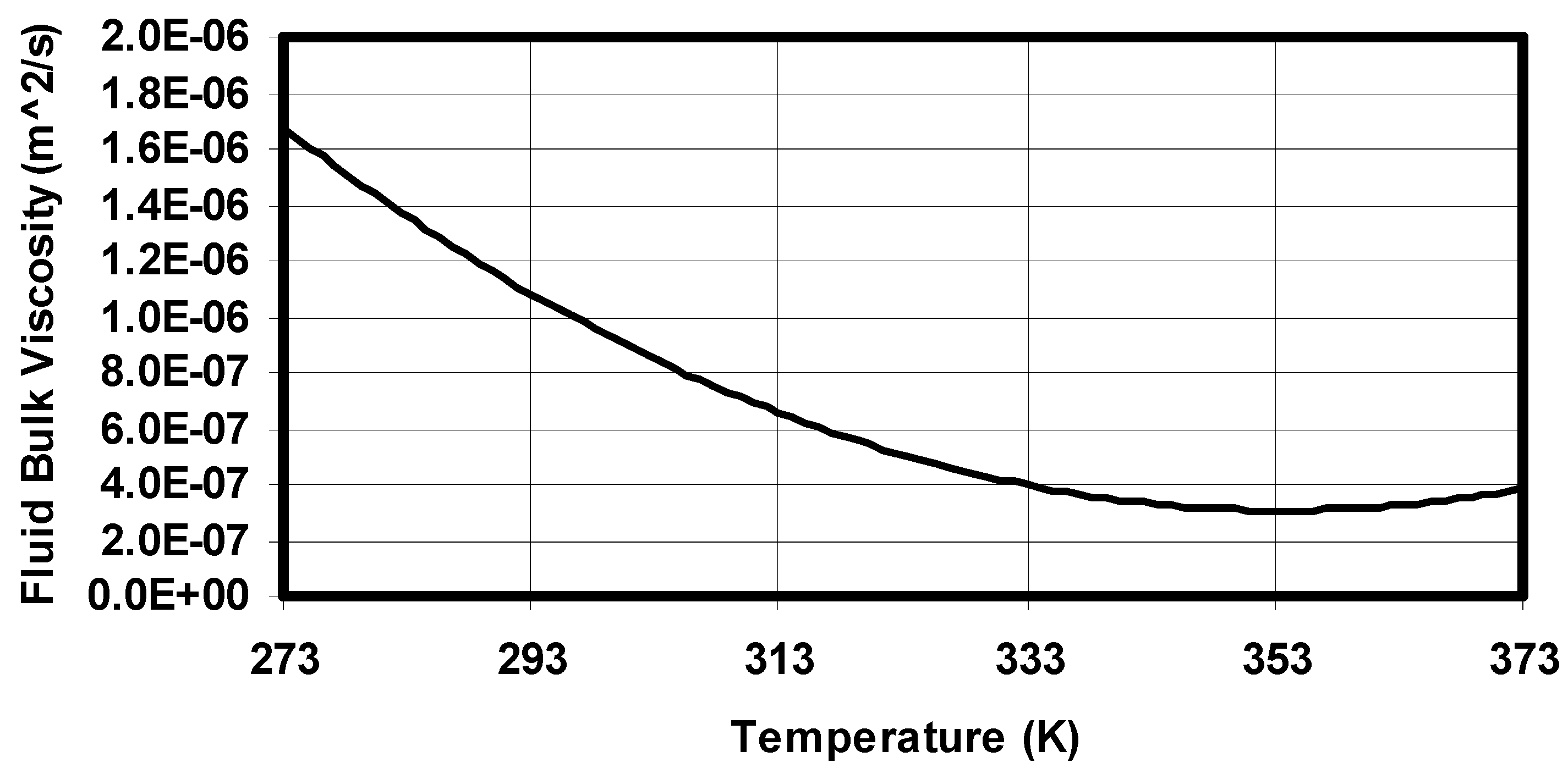
Figure 2 shows the temperature dependent fluid bulk viscosity. In this case, increasing fluid temperature reduces the viscosity and it remains almost the same as the temperature increases beyond 350 K.
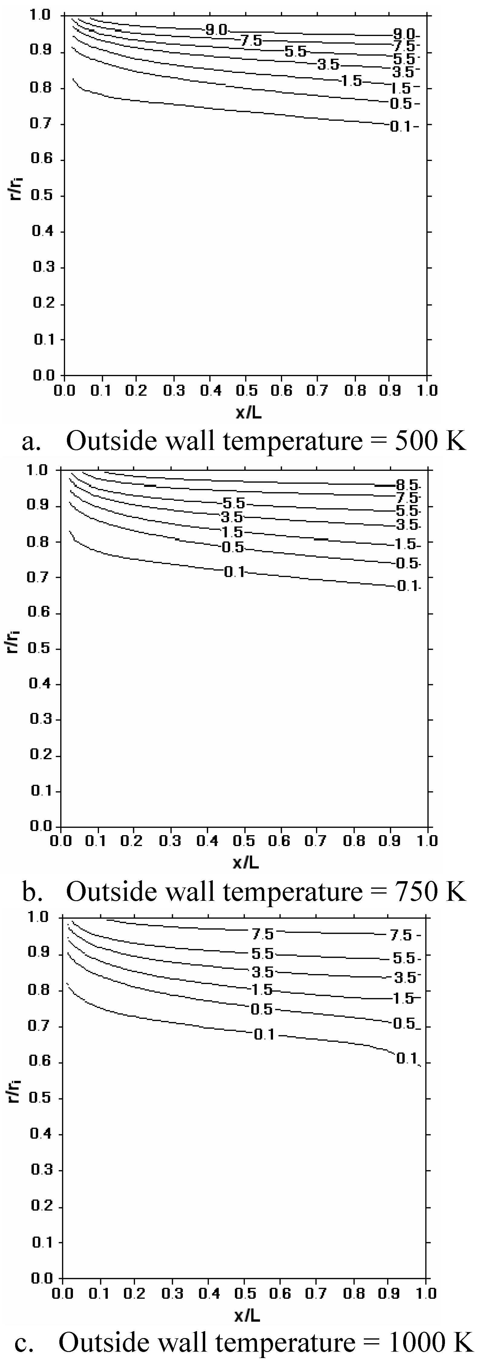
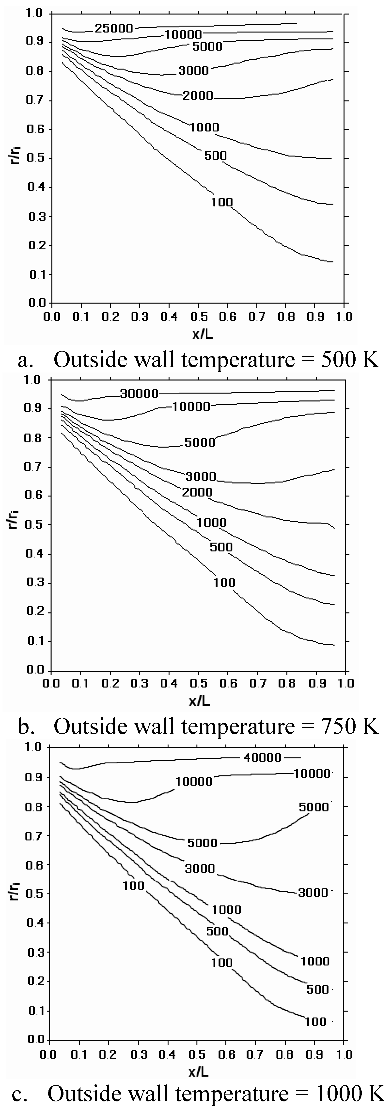
Figure 3 shows the dimensionless temperature contours in the fluid for three pipe wall temperatures. Dimensionless temperature contour distribution appears to be similar for all pipe wall temperatures. This is because of the constant fluid properties, despite the heat transfer rates due to different wall temperatures are different, i.e. dimensionalizing the fluid temperature eliminates the influence of heat transfer rates on the temperature distribution. Moreover, temperature contours attain high values in the surface region and as the distance from the pipe wall towards the pipe center increases, its magnitude reduces. This is more pronounced at the pipe exit.
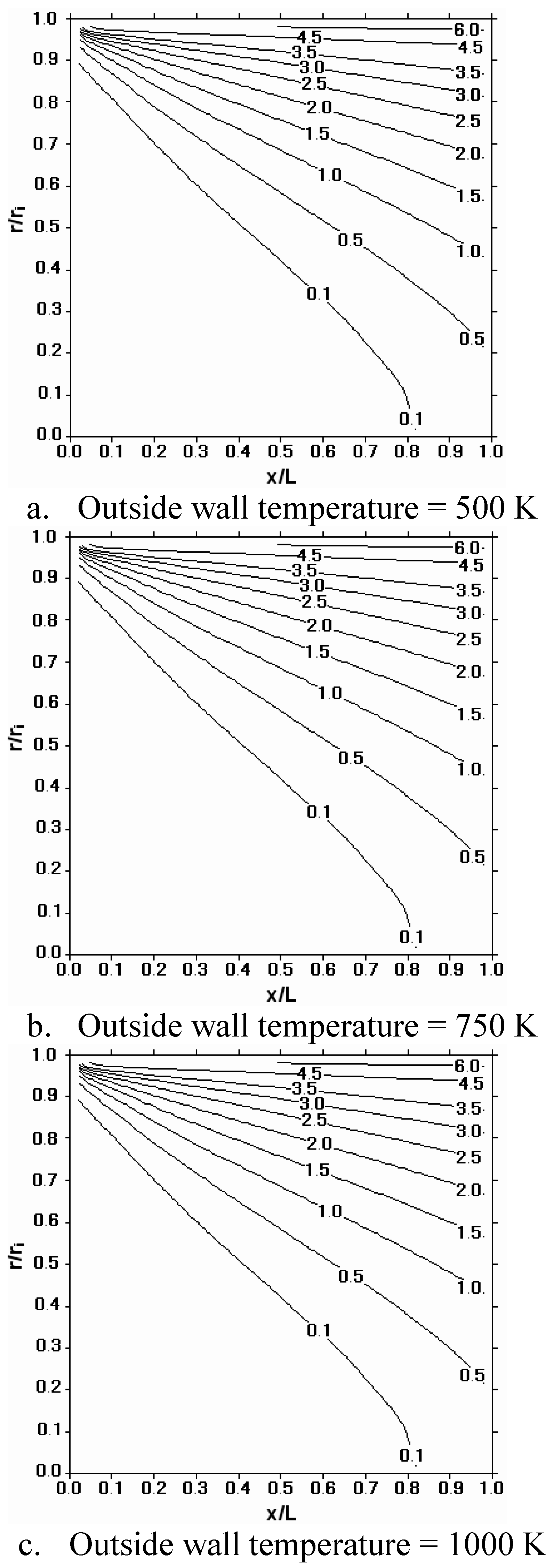
Figure 4 shows entropy contours for constant viscosity case and different pipe wall temperatures. Entropy generation is high in the region close to the pipe wall, which is due to the attainment of high temperature gradients in this region, i.e. high temperature gradient results in high entropy generation rate (equation 10). It should be noted that entropy generation rate due to fluid friction is lower than that due to heat transfer [
19]. Entropy contours extends towards the symmetry axis at the pipe exit. In this case, entropy contours follow almost the temperature contours in the fluid. Entropy contours close to the pipe wall change considerably for different pipe wall temperatures. This is because of the different magnitude of temperature gradient developed in this region.
Figure 5 shows temperature contours due to variable viscosity case for three outer pipe wall temperatures. As the wall temperature increases, temperature contours expand towards the fluid bulk, which is more pronounced towards the pipe exit. This is because of the convective heat transfer from the pipe wall to the fluid. Moreover, the influence of variable viscosity on the temperature contours is significant, which can be observed after comparing
figure 3 and
figure 5. In this case, heating of the fluid in the region close to the wall is more pronounced for variable viscosity case. Consequently, increasing fluid temperature close to the pipe wall reduces the fluid viscosity, which in turn lowers the heat transfer in the fluid towards the symmetry axis.
Figure 6 shows entropy contours for variable bulk viscosity case and different pipe wall temperatures. In the case of variable properties, entropy contours attained considerably higher values in the region close to the pipe wall as compared to those corresponding to constant viscosity case (
figure 4). This occurs because of the high temperature gradient, in which case, variable viscosity modifies the temperature distribution in this region and resulting in high temperature gradients. Consequently, entropy generation due to temperature filed enhances. Entropy generation at pipe inlet and at pipe exit does not vary considerably as compared to that occurring for the constant viscosity case. The magnitude of the entropy generation increases as the pipe wall temperature increases. This suggests that high temperature gradients due to high pipe wall temperature results in high rate of entropy generation in the region close to the pipe wall
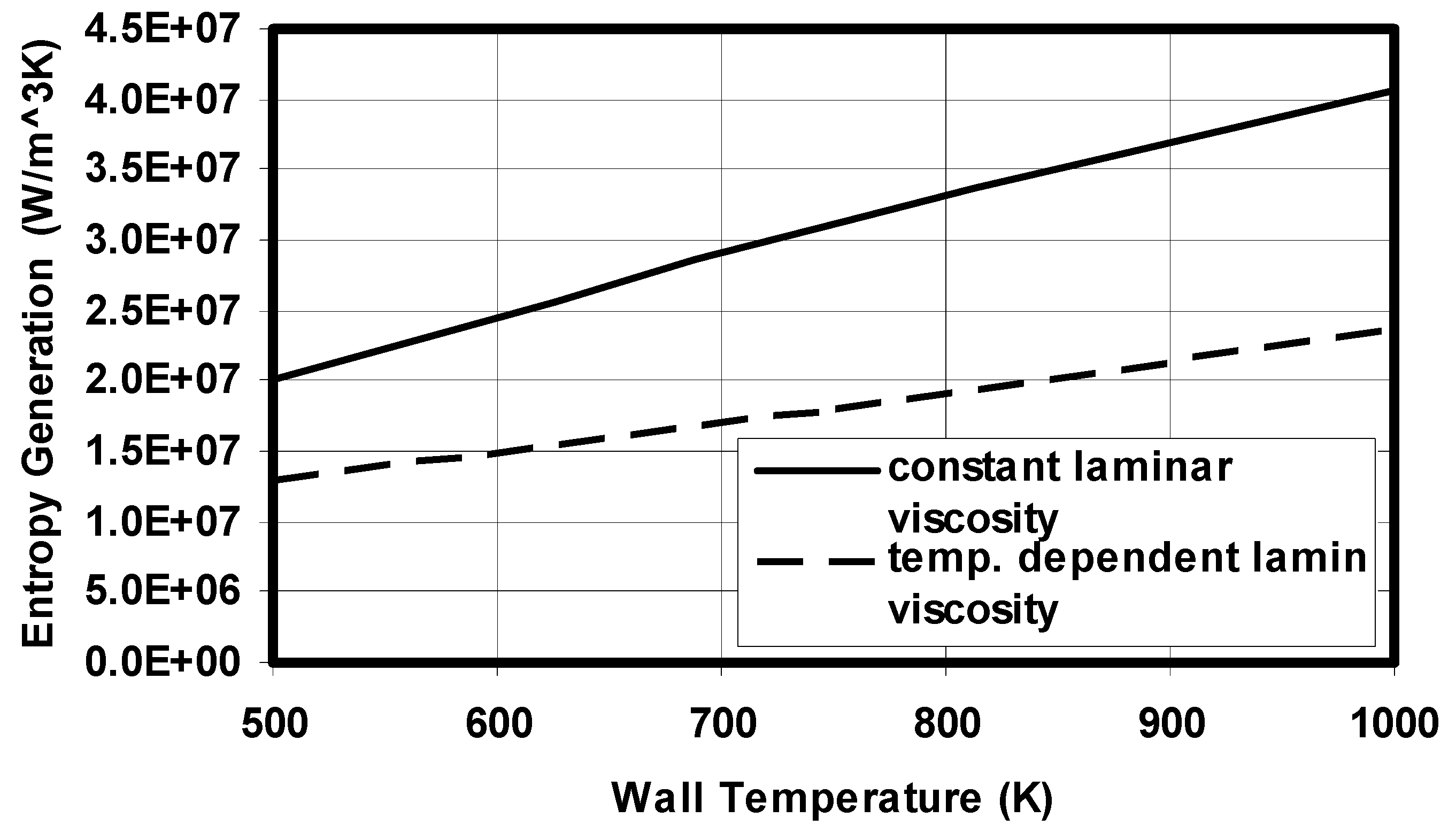
Figure 7 shows rate of entropy generation in the fluid with pipe wall temperature for constant and temperature dependent viscosity cases. In general, increasing pipe wall temperature enhances the rate of entropy generation in the fluid. Although entropy generation rate attains high values in the region close to the pipe wall for the variable viscosity case, the total entropy generation is lower than that corresponding to constant viscosity case. This is because of the extension of the high temperature gradient in the fluid, i.e. temperature gradient is high in the region close to the wall for variable properties case; however, high temperature gradient region extends further into the fluid for the constant viscosity case.
Conclusions
The influence of fluid viscosity on the entropy generation rate is investigated in the pipe flow at different wall temperatures. The temperature and flow fields are computed numerically using the control volume method. It is found that fluid viscosity influences considerably temperature distribution in the fluid close to the pipe wall. In this case, the high temperature gradients extend further towards the pipe center for constant properties case. On the other hand, variable properties reduce the size of the region, where the high temperature gradients occurs in the flow field. Entropy contours follow almost the temperature contours. Moreover, volumetric entropy generation rate is higher in the region close to the pipe wall for variable properties case. The total entropy generation rate is higher for constant properties case as compared to its counterpart corresponding to the variable properties case. Volumetric entropy generation rates at pipe inlet and exit do not vary considerably for variable viscosity case; however, the opposite is true for constant viscosity case. Increasing pipe wall temperature enhances the rate of entropy generation.


