1. Introduction
Methane is a potent greenhouse gas that is of importance in discussions about climate and energy. Both natural and anthropogenic sources of methane are of interest to the atmospheric science community. It is well known that natural methane sources are often spatially heterogeneous [
1], which makes large area monitoring and the ability for spatial identification of increasing importance. Currently there are multiple technologies used to monitor atmospheric methane concentrations and the most accurate and widely accepted in the atmospheric research community are optical sensing technologies based on single location (extractive or open-path) laser absorption spectrometers [
2,
3]. While these techniques offer high sensitivities, the lack of spatial information limits their ability to identify sources or sinks without large infrastructures of multiple, often costly, sensor nodes. To address this need, a remote, multi-path sensor was designed, characterized [
4], and deployed in the field. The results of this first field test were to illustrate the capability of this sensing configuration and indicate needs for further technology development. Use of a centralized system allows for distribution of the spectrometer cost over multiple sensing paths, effectively eliminating the need for a network of multiple sensor nodes. The location for this field campaign was Sallie’s Fen Environmental Station (SFES), a site monitored for methane emissions by the University of New Hampshire for more than two decades [
5,
6,
7,
8]. This long-term record of methane emissions and also meteorological variables measured at this wetland, located in Barrington, NH (43°12.5′ N, 71°3.5′ W), make this site well suited for studies of methane from wetland sources. Wetlands are the largest natural emitters of methane [
8], and thus SFES is an important representative ecosystem and provides an excellent testing platform for evaluation of a new instrument.
2. Spectroscopic Sensing System
A technique known as Chirped Laser Dispersion Spectroscopy (CLaDS) was recently developed to address some of the key issues in traditional absorption-based, remote sensing techniques; namely the dependence of the measured signal amplitude on the received power and the linearity and dynamic range of concentration detection are significantly improved with CLaDS [
9,
10]. CLaDS takes advantage of measuring the optical dispersion induced by interaction of the laser light with the targeted species. This is achieved by probing the sample transition with a frequency-chirped, multi-color, coherent laser beam. Since each component wave (color) experiences a different index of refraction related to the dispersion profile of the molecular transition, the sample dispersion can be extracted through analysis of the instantaneous frequency of the heterodyne beat note generated by the component waves on a square-law photodetector. Unlike an absorption measurement, which is based on quantification of transmitted light intensity, a dispersion measurement is determined from the phase of the detected light and thus is fundamentally independent of the received optical power [
11]. Key benefits of CLaDS, such as immunity of the CLaDS signal to intensity fluctuations, and a linear response with concentration [
12], are achieved while still maintaining sensitivities needed for environmental trace gas monitoring [
13]. All of these qualities are essential for open-path measurements where atmospheric conditions can vary drastically resulting in strong fluctuations of the intensity of the light received on the photodetector (e.g., due to fog or dust). To provide continuous monitoring functionality through spectral line-locking to the target transition, a variant of CLaDS technique, called Chirp Modulated (CM) CLaDS [
11] was employed in this instrument.
In a recent work, the feasibility of CLaDS operation in the near-infrared was demonstrated, showing the use of both single sideband (SSB) and double sideband (DSB) modulation of the optical carrier used for generation of CLaDS signals [
14]. The instrument core developed for this field campaign was detailed in a previous publication (see [
4]) and utilized DSB CM-CLaDS to target methane in the near-IR at 6046 cm
−1 (1653 nm).
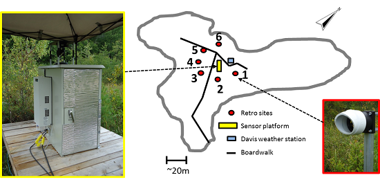
Figure 1.
Chirped Laser Dispersion Spectroscopy (CLaDS) methane instrument installed in a weatherized enclosure; the inset shows a close-up of the optical port and a computer-controlled gimbal mount used to direct light horizontally to different sections of the fen.
Figure 1.
Chirped Laser Dispersion Spectroscopy (CLaDS) methane instrument installed in a weatherized enclosure; the inset shows a close-up of the optical port and a computer-controlled gimbal mount used to direct light horizontally to different sections of the fen.
Prior to the field deployment, the system was installed in a weatherized, temperature-controlled cabinet (manufacturer: DDB Unlimited), shown in
Figure 1. A sealed polycarbonate window was installed in the top of the cabinet to allow the laser light to be launched from inside the enclosure with negligible transmission loss (see inset in
Figure 1). A gimbal mounted mirror system was used to direct the laser radiation to multiple retroreflectors located at a given distance away from the sensor cabinet. The system was characterized in ambient methane conditions prior to installation at SFES. With the assumption that the atmospheric methane concentration was constant during the test, a path-length and bandwidth normalized detection limit of 1.7 ppm-m-Hz
−1/2 was achieved (Allan Deviation is shown in
Figure 2), which was consistent with the specifications of the laboratory prototype tested earlier [
4].
Figure 2.
Allan Deviation analysis performed in the ambient methane conditions prior to transportation to Sallie’s Fen Environmental Station (SFES) shows a detection limit of 1.7 ppm-m-Hz−1/2 and system drift dominated performance for averaging times >100 s.
Figure 2.
Allan Deviation analysis performed in the ambient methane conditions prior to transportation to Sallie’s Fen Environmental Station (SFES) shows a detection limit of 1.7 ppm-m-Hz−1/2 and system drift dominated performance for averaging times >100 s.
For the experiments shown in [
4], the R3 transition in the 2ν
3 band of methane at 6046 cm
−1 (1653 nm) was used. Due to spectral interference from water vapor, we switched to the R4 transition in the same band at 6057 cm
−1 (1651 nm), which provided better conditions for atmospheric open path measurements (the diode laser was operated at 5 °C instead of 25 °C used in [
4]). This is illustrated in
Figure 3, which shows the simulated CLaDS spectra for methane (CH
4), water vapor (H
2O), and carbon dioxide (CO
2) around 6057 cm
−1 based on the HITRAN 2008 database [
15]. The cross-sensitivity of the CLaDS signal amplitude to atmospheric water concentration for the two CH
4 lines is shown in
Figure 3b, and clearly shows the influence of the close-by water transition on measurements performed at 6046 cm
−1.
Figure 3.
(a) Simulated CLaDS spectra of the three main atmospheric species in the 1651 nm (6057 cm−1) region; (b) Impact of the water vapor concentration on the peak amplitude of the CH4 CLaDS signal calculated for the transitions at 6057 and 6046 cm−1 (both have similar linewidths, thus double sideband (DSB) spacing of Ω = 1.2 GHz was used for calculating the CLaDS signal in both cases).
3. Deployment Details
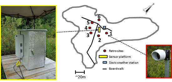
The CLaDS sensor was installed at SFES in late June 2013 with a sensing configuration as illustrated in
Figure 4. Six 2-inch retro-reflectors were mounted in a star-like configuration ~20 m away from the sensor cabinet, and the locations were chosen to sample CH
4 emissions from areas with different plant species. It should be noted that this distance of 20 m is not a maximum target distance, but was rather chosen to sample a certain area within the fen. The path length for each retro-reflector location was precisely measured and stored to be used in calculating the average methane concentration along each path. During the deployment each optical path was probed for two minutes, after which the gimbal position was changed to target the next reflector in the cycle.
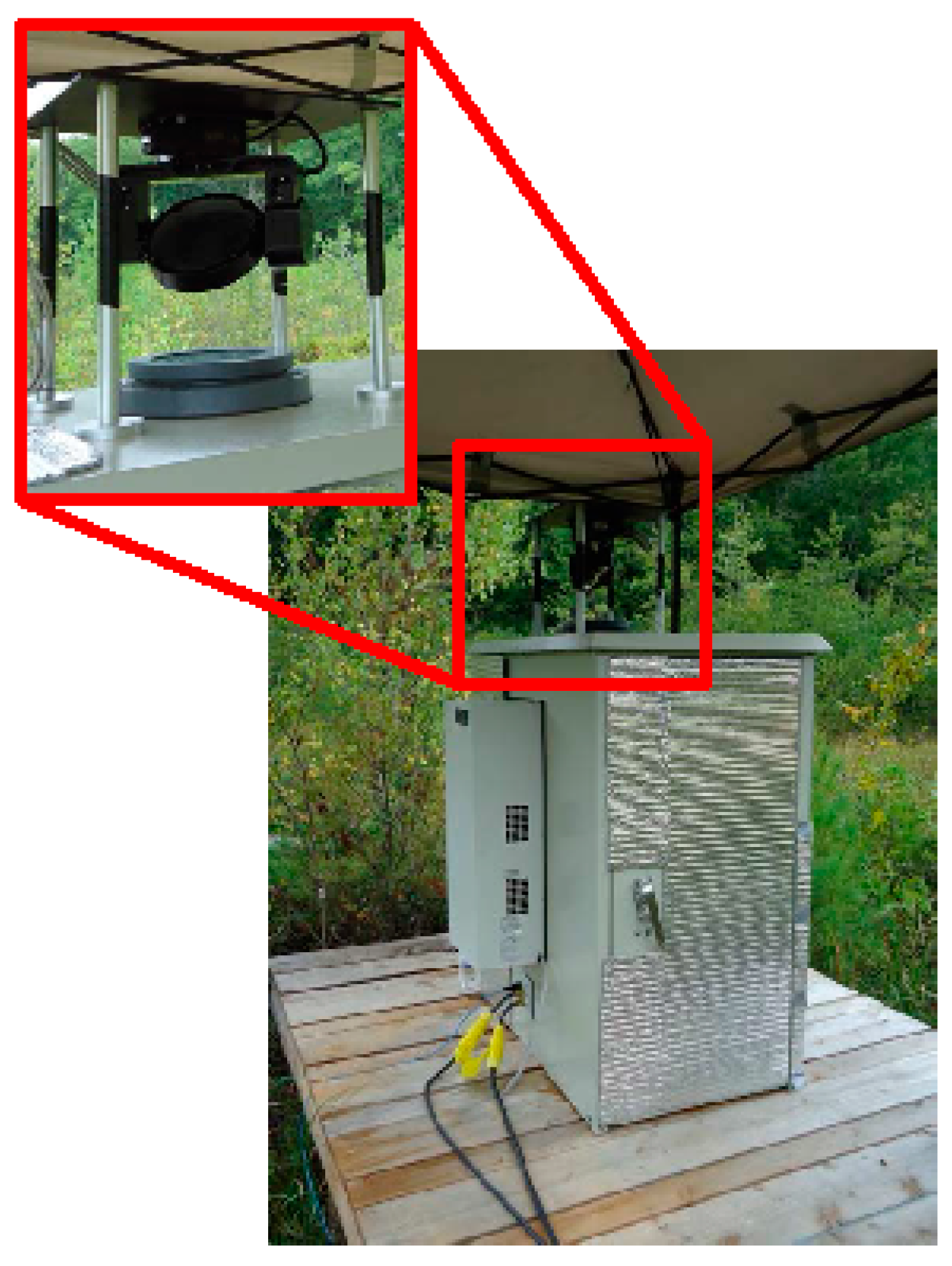
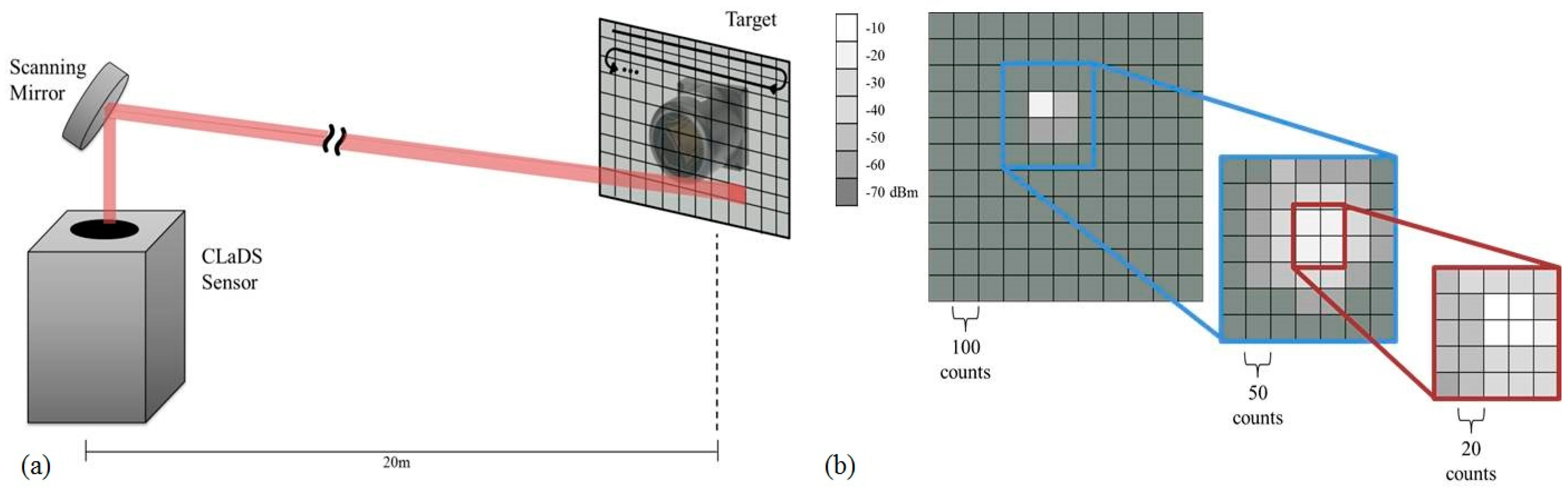
The sensor platform and the retroreflector posts were affixed to the relatively unstable wetland surface, making it quite challenging to provide a stable optical alignment with the retroreflectors. To address this issue we developed an active alignment procedure with raster-scanning algorithms to realign the system before each two-minute sampling interval as well as aid in the initial alignment of the system (see
Figure 5). Initial alignment of the system optics was performed using the scheme outlined in
Figure 5b. A large grid and step size (11 × 11, 100 counts) was used for a rough alignment. The maximum of this scan was used as the center of another scan with smaller settings (7 × 7, 50 counts). Subsequently, the maximum of this scan was used as the center for fine tuning of the alignment (5 × 5, 20 counts). Once the maximum return signal position was identified the alignment algorithm set the mirror position at the same coordinates and the methane monitoring was initiated (the alignment algorithm was programmed to eliminate the effects of backlash from the gimbal motors). During the measurement cycle, if the return powers dropped below a set threshold, a raster scan was initiated at a small grid and step size settings (5 × 5, 20 counts). If after this first scan return powers did not meet the threshold condition, a second raster scan at larger settings (11 × 11, 100 counts) was performed. If again the threshold condition was not met, that path was flagged in the software as needing attention by a human operator.
Figure 4.
The sensor configuration deployed at SFES. The yellow rectangle, red circles, and the blue square represent the central sensor platform, the location of the six retro-reflectors, and the weather station, respectively. The image shows the mounting of the retro-reflector onto fence posts which were inserted several feet into the fen surface.
Figure 5.
Raster algorithm used to optimize the scanning mirror position. (a) Configuration for the retro-reflector searching scheme; (b) Consecutive scans of decreasing grid size (11 × 11, 7 × 7, 5 × 5) and step size (100, 50, 20 counts) used maximize the return beatnote powers (in dBm) to the CLaDS sensor during initial position calibration.
A weather station (Davis Vantage Pro2, Barrington, NH, USA) was mounted several meters away from the cabinet and provided meteorological data (temperature, pressure, relative humidity, and wind speed and direction) collected with the methane signals. A 10 × 10 foot canopy was installed over the sensor platform to protect the setup from rain and to prevent direct sunlight from heating the cabinet. Optical powers of less than 1 mW were launched from the sensor with a divergent beam, making the sensing configuration eye-safe [
16]. The system began collecting data in late July (30 July 2013) and continued until mid-October (21 October 2013), with a 3-week break in late August when the gimbal mount malfunctioned and was sent out for repairs.
Signal Calibration in Field Conditions
In order to ensure the system accuracy did not deteriorate during the deployment, a fiber-coupled gas cell (3 cm long and filled with 19.4% of methane in nitrogen at 740 Torr) was placed inside the cabinet to enable periodic re-calibration [
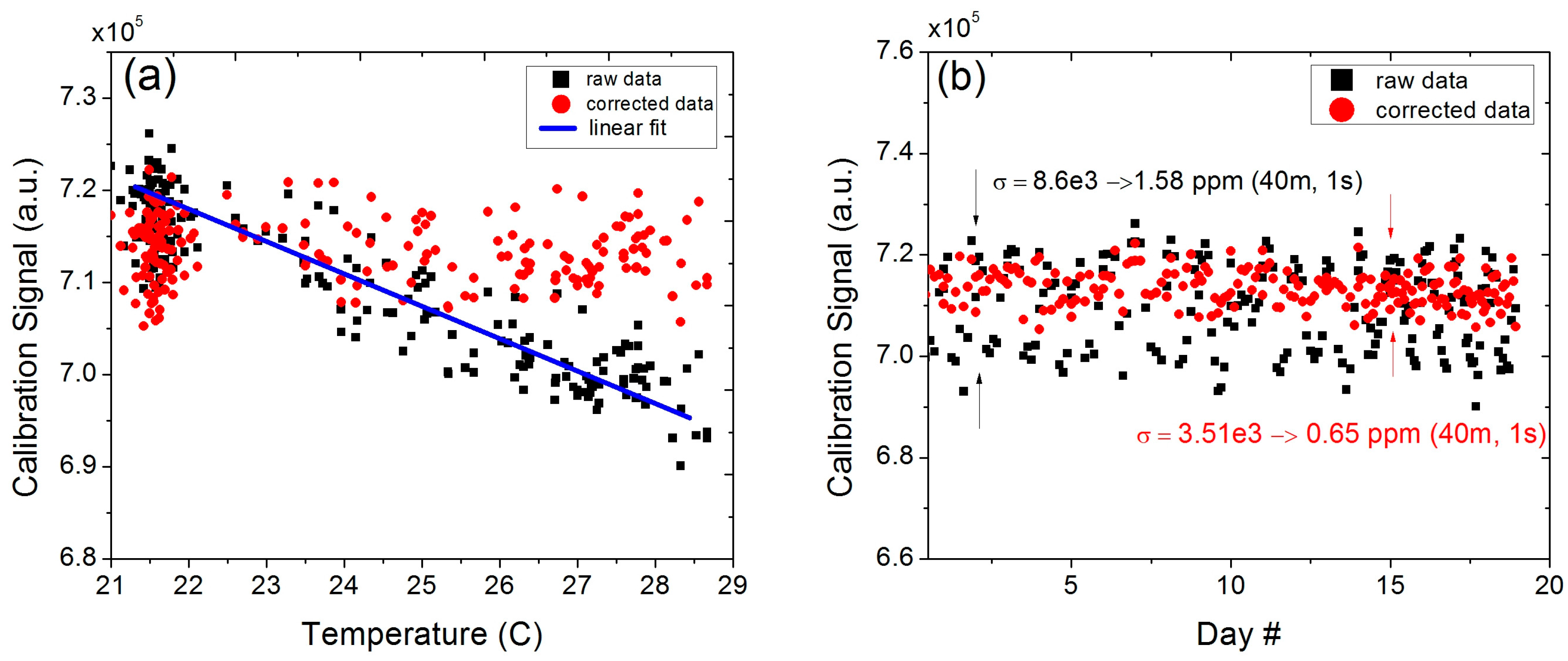
4]. Despite being housed in an air-conditioned cabinet, the system experienced relatively larger temperature swings than planned (more than 7 °C) due to the limited functionality (lack of heating mode in the cool nights) and a moderate cooling capacity (4000 BTU) of the built-in air conditioning unit. As a result of the varying temperature in the cabinet, the raw calibration signal showed a clear temperature dependence (see
Figure 6). Direct application of this raw calibration signal to the conversion of the acquired open-path data into concentration levels would introduce a large amount of error into the retrieved values.
Figure 6.
(a) Temperature dependence of the calibration signal as a result of larger temperature swings within the weatherized enclosure and the data corrected with by the temperature-dependent spectral model; (b) Calibration signals over the course of 19 days before and after temperature correction.
To suppress the effects of cabinet temperature fluctuations, the raw calibration signal was corrected for both the temperature dependence of the molecular transition as well as for the temperature induced pressure changes within the sealed gas cell. The internal cabinet temperature was monitored continuously with the Davis Vantage Pro2 console temperature sensor and the data was used for correction of the calibration signal. The temperature correction of line intensity was determined using the following expression [
17].
where
T is the temperature (K),
is the spectral line intensity [cm
−1/(molecule cm
−2)],
is the total internal partition function,
c2 is the second radiation constant (1.4388 cm·K),
is the lower state energy of the targeted transitions (cm
−1), and
is the line frequency (cm
−1). The above expression was used in conjunction with molecular parameters from the HITRAN documentation [
18] to correct the change in line strength due to the deviation in temperature away from the reference temperature
used in HITRAN (usually a reference temperature and pressure of
Tref = 296 K and
pref = 1 atm are used).
The effects of the change in pressure within the sealed cell were addressed using the ideal gas law in isovolumetric conditions yielding
where
p and
T are actual temperature and pressure in the cell (in (atm) and (K) respectively), and
p0 and
T0 are the nominal values provided by the manufacturer of the gas cell. The calculation of the actual pressure is performed based on the temperature measurements inside the sensor cabinet. Both temperature and pressure values were used to correct the pressure broadened halfwidth (cm
−1/atm) according to [
17],
where the calculated pressure
and the measured temperature were used. In Equation (3), the parameter
is the air-broadened HWHM (cm
−1),
is the self-broadened HWHM (cm
−1),
is the partial pressure (atm), and
n is the coefficient of temperature dependence. Equations (1)–(3) were used to model the CM-CLaDS spectrum, and the peak amplitude of the reference signal was used for calibration of the open-path data acquired in a line-locked mode (see [
4] for details on the sensor mode of operation). Temperature fluctuations not only affected the calibration channel, but also impacted the precision of the sample channel. In-laboratory testing of the system prior to the field test showed that the main source of drift in long-term measurements was a parasitic fringe between the photodetector window and the telescope body [
4]. In the field, when the collection optics were subjected to these large temperatures swings, the effects of the fringe were amplified. From analyzing the noise in the sample channel signals, the estimated precision under these field conditions was determined to be 0.2 ppm (over 40 m and in 1 s). This approximately represents a 5× degradation in system performance; however, despite this increase in fringe noise, the probed path lengths provided enough signal to investigate the feasibility of various sensing configurations in the field.
5. Conclusions
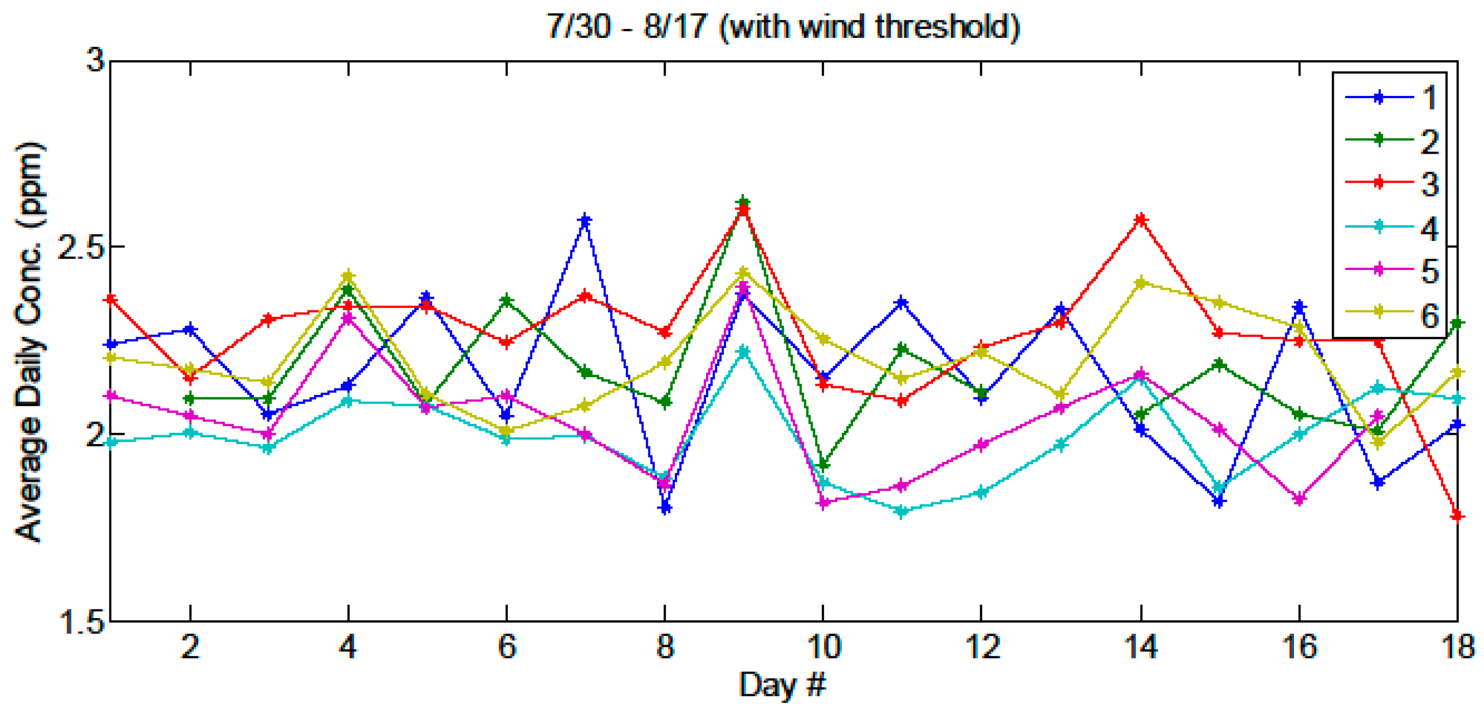
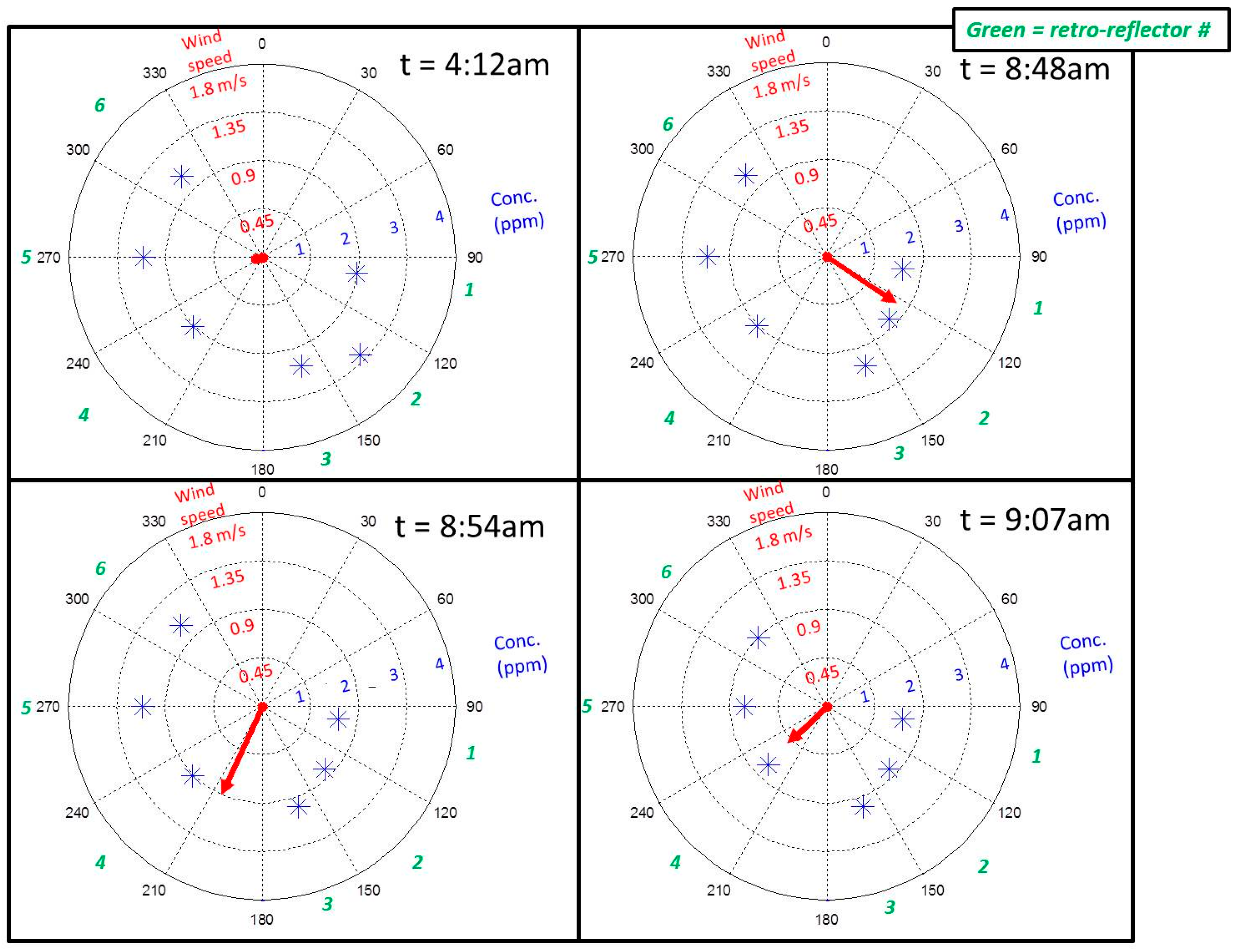
In this work we demonstrated the feasibility of a CM-CLaDS system for open-path sensing of atmospheric methane over multiple sampling paths covering a large area footprint. Operation in the field at SFES provided a challenging environment to test the functionality and robustness of the instrument. A dedicated spectroscopic reference data correction was developed to provide robust calibration of the instrument in the presence of temperature fluctuations within the sensor enclosure. We have also shown that despite operating in a challenging environment with an unstable wetland floor, we have been able to mitigate the opto-mechanical stability issues with a fully automated optical alignment system. In addition, parasitic etalons from the collection optics (i.e., the telescope and detector), were found to be the limiting source of signal drift in our system, and deteriorated the system performance by ~5× with respect to laboratory setting. Despite these challenges, we were able to demonstrate the ability of a remote, multiple-path sensor for investigation of larger-scale methane trends; such as diurnal cycles, the influence of wind dynamics and transport, as well as emissions from different sample paths of various plant species. Further improvements to the sensor will involve a redesign of the free space optics to minimize unwanted interference effects, customization of the sensor electronics to increase functionality and decrease the amount of waste heat within the sensor enclosure.


