The NEP instrument configuration is similar to the space accelerometer for gravitation experimentation (SAGE) developed for the on-orbit MicroSCOPE mission [
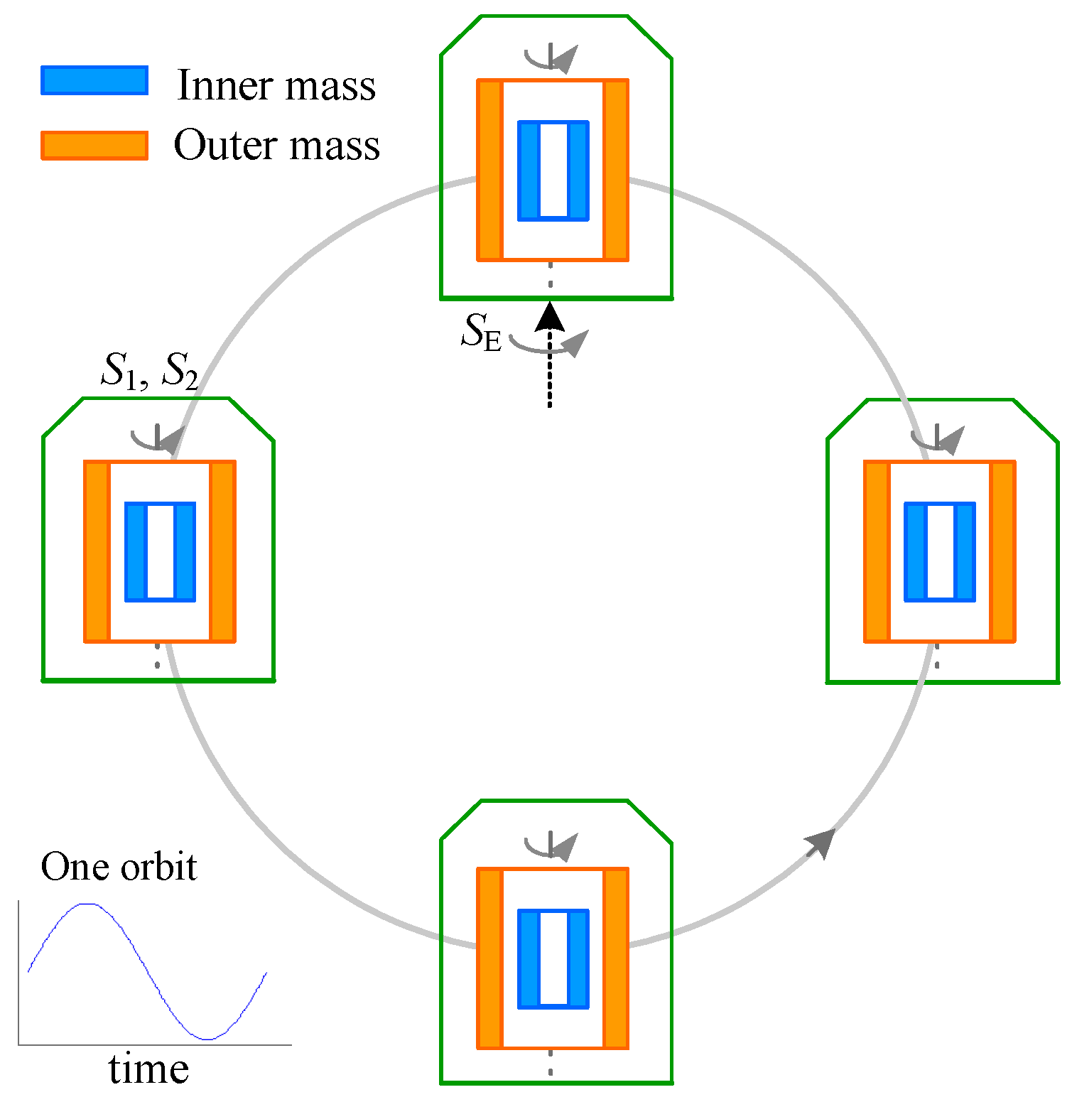
17]. In this weak equivalent principle (WEP) test, free fall motion of two non-spinning test masses which are composed of different materials is observed when both masses are subjected exactly to the same gravitational field. In comparison to the MicroSCOPE mission [
3], the proposed NEP experiment aims to verify the spin-spin interaction between rotating extended bodies and the Earth. Hence, two TMs of the differential NEP accelerometer are made of the same material but rotated with much different angular momenta. The most challenging aspect in design of the NEP instrument is that the two TMs are spinning during on-orbit tests, such as 10
4 rpm for the inner TM and 100 rpm for the outer TM. During operation there is no any physical contact on the TMs to enable continuous rotation of the inner and outer masses. In this case, the thin gold wire scheme commonly used in traditional space accelerometers, which enables the position detection and permits the control of the electric charge of the mass [
18], is not applicable to the NEP accelerometer. Therefore, the NEP instrument design is significantly different from previous EP instruments, such as SAGE. A comparison among the NEP instrument and two similar inertial sensors are listed in
Table 1. The continuous rotation of the two TMs makes the NEP instrument design more complicated, especially in the sensor unit and rotation control electronics.
3.1. Sensor Unit
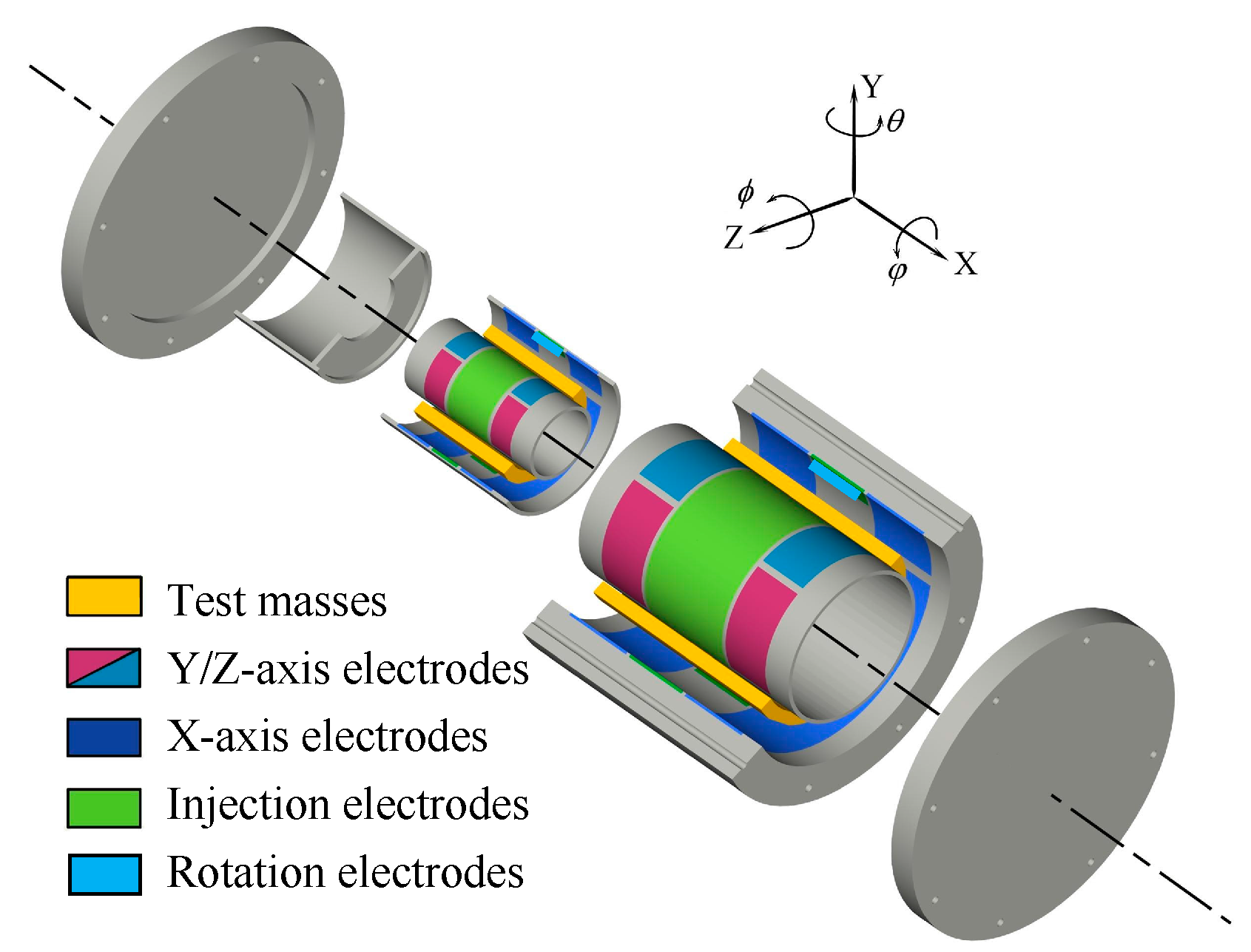
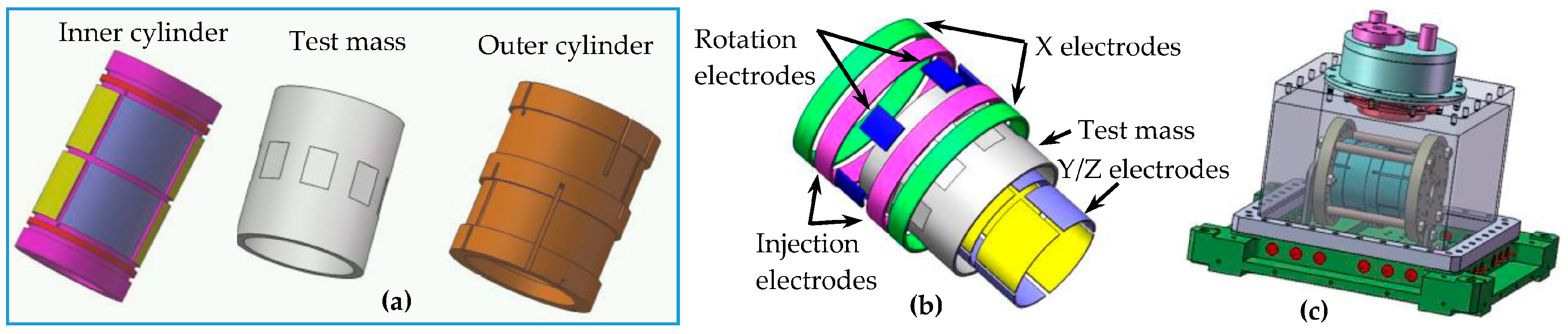
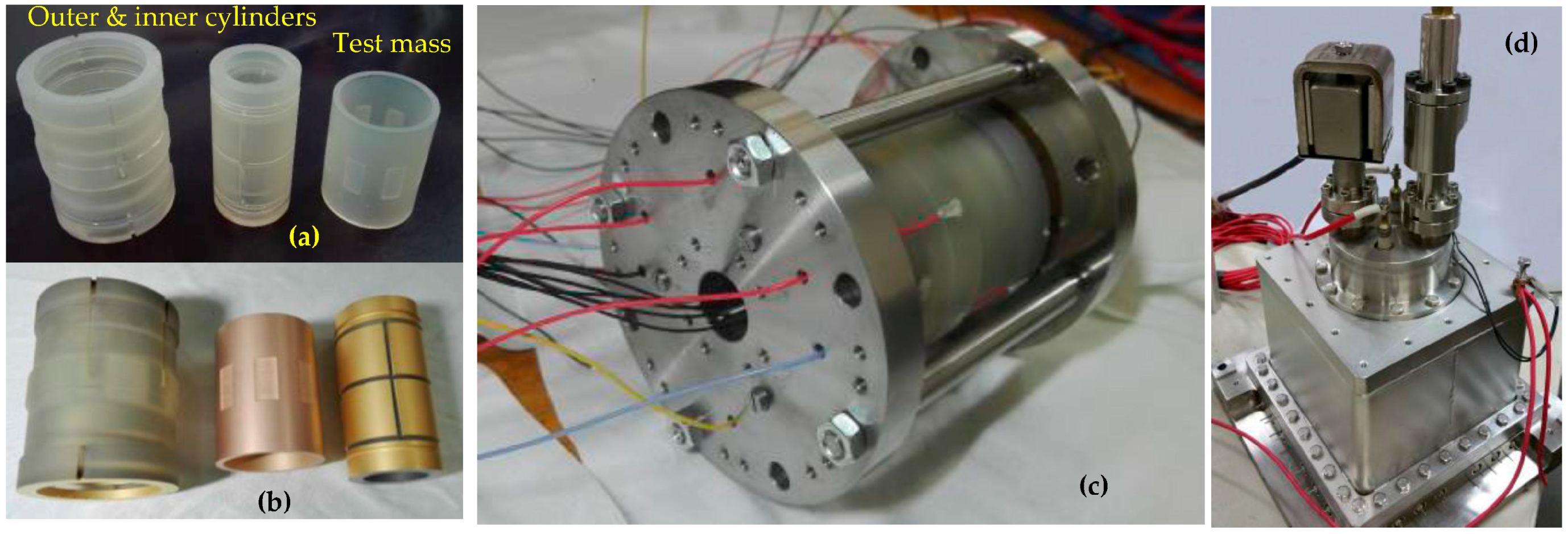
This differential accelerometer is specifically optimized for the space test of the NEP. The mechanical core of the NEP instrument contains two concentric inertial sensors, each composed of one hollow quasi-cylindrical TM and two concentric electrode cylinders which are positioned within and without the mass, as shown in
Figure 3. The material of the two masses has been selected to titanium alloy by taking into account of the purity, specific gravity, homogeneity, machining ability, thermal stability, electrical conductivity and magnetic susceptibility. Given that the two TMs are not idealized point masses, a common center of mass is not sufficient to guarantee both bodies will be subjected to the same force. Therefore, the cylinder dimensions should be carefully designed to approximate the monopole property and thus reduce the effects of local gravity gradient fluctuations [
17,
22]. This effect can be minimized by design of the TM dimensions with equal moments of inertia on each axis, which has been carefully considered and adopted by several WEP missions [
3,
4]. Moreover, to further minimize the gravity gradient effects on the NEP signal, the off-centering between the two TMs is expected to be less than 20 μm after the instrument fabrication and integration [
3]. The two TMs are initially designed by modeling and optimization of overall suspension and rotation performances, as listed in
Table 2.
Each test mass is surrounded by two gold coated cylinders made of ultra-low expansion (ULE) glass ceramic, exhibiting a 1.6 × 10
−7/°C coefficient of thermal expansion at 25 °C. Associated with high thermal stability of the instrument interfaces, it ensures a very steady set of electrical conductors around the mass [
3]. The necessary electrodes on two cylinders are defined by gold coating to function as capacitive position sensing, electrostatic suspension and rotation control of the mass, as depicted in
Figure 4. As the electrostatic force is always attractive, the actuation electrodes act in pairs to provide both a positive and a negative force for any degree of freedom. On the inner cylinder, there are four quadrant electrodes (Z
1+, Z
1−, Z
2+, Z
2−) for the radial
z- and
-axes suspension and other four quadrant electrodes (Y
1+, Y
1−, Y
2+, Y
2−) for the radial
y- and
θ-axes, respectively. Moreover, to enable the capacitive position detection, a sinusoidal excitation voltage is applied to the TM via one common injection electrode (INJ). On the outer cylinder, there are four axial electrodes (X
1+, X
1−, X
2+, X
2−) around the entire circumference, as well as a ring of six stator electrodes for rotation control around the
x direction. The rotation operation around the
x-axis is based on the principle of variable-capacitance electrostatic motors [
21]. Note that the
x-axis accelerometer provides the most sensitive measurements, which are utilized to test gravitational effects of the spinning mass. Therefore, along the axial sensitive direction, the configuration is such that the gradients of capacitances between the electrodes and the mass are quite independent of the position of the TM, which doesn’t induce the first-order electrostatic negative stiffness [
22]. Likewise, the corresponding geometry parameters of the four electrode cylinders are listed in
Table 3. The four cylinders of the two inertial sensors will be integrated on a unique ULE centering part, serving as a reference frame for the NEP instrument.
3.2. Electrostatic Suspension
This electrostatic accelerometer is based on the force-balance technology which measures the electrostatic force necessary to maintain the TM motionless with respect to the sensor cage [
22]. The motion of each TM with respect to highly stable instrument frame is actively servo-controlled by electrostatic suspension in five DoFs: translations along the
x,
y and
z axes, and rotations around two in-plane axe,
θ and
ϕ, respectively.
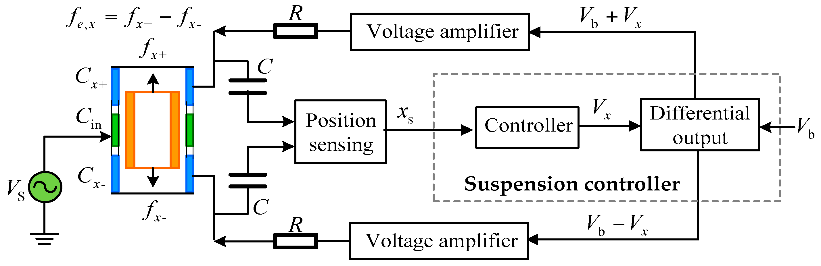
Figure 5 shows a schematic diagram of the electrostatic suspension loop for the
x axis. A sinusoidal carrier signal
(~100 kHz) is applied to the injection electrode which is utilized to capacitively couple the excitation signal to the TM for capacitive position sensing [
23]. In the presence of external force, the TM displaces away from its nominal position, resulting in a change in the differential capacitance,
, between the TM and a pair of top and bottom suspension electrodes. The position sensor senses this capacitance change and then feeds the position signal
into a feedback controller to stabilize the suspension servo loop. In order to linearize the electrostatic feedback force, the suspension system is normally operated in a differential fashion so that the voltage on the positive electrode is the sum of a bias voltage
and a control voltage
while the voltage on the negative electrode is produced by subtracting the bias voltage from the control voltage. Finally, the feedback voltages from two voltage amplifiers are applied on the suspension electrodes by which the the electrostatic force is generated to balance the external force, pulling the TM back to its nominal position. The resultant feedback forces are derived from the accurate measurement of the applied voltages on the pairs of electrodes. Note that these suspension electrodes function in pairs to simultaneously measure and control the TM position, with the complete set providing contactless electrostatic suspension in five DoFs. The RC networks shown in
Figure 5 are used to separate relatively low frequency forcing voltages from high frequency position sensing signals.
Adequate suspension stiffness and precise centering control of the TM are important to ensure desirable performance of the force-balanced electrostatic accelerometer. To stabilize the movement of each TM, we need to control its motion in five DoFs. If all the cross-coupling effects among the different axes are ignored by assuming small position deviation, the dynamics of the TM can be modeled by five uncoupled 1-DoF systems:
where
and
are the mass and moment of inertia of the TM,
and
the linear and angular displacements of the TM away from its equilibrium position,
and
the electrostatic feedback force and torque,
and
the externally applied input force and torque, the subscript
denotes the axis along which the force is produced and
denotes the axis around which the torque is produced, respectively. The residual air-film damping effect is neglected in Equation (2) by considering that the TM is suspended in high vacuum.
For instance, the electric force produced by the charged set of the feedback electrodes on the mass along the considered
x-axis can be linearized as [
24]:
where
is the actuator gain and
the position stiffness or negative spring constant, respectively. The maximum electric force applied on the centered TM is
by considering the condition
holds. Note that the
x-axis suspension design is optimized to generate weak electrostatic force by using an area variation scheme [
18]. In principle, it is free of the negative position stiffness, i.e.,
. On the other hand, the position stiffness has a significant effect on other four suspension axes in which a gap variation scheme is utilized to generate relatively large electrostatic force in order to balance possible disturbance resulted from the TM spinning.
This linear model is valid by assuming that the motion of the PM is very small, e.g., in a range less than 10% of the nominal gap. This assumption can be ensured by adequate suspension stiffness provided through design of the suspension control loop. Substituting Equation (3) into Equation (2a) and then taking the Laplace transform yield the dynamics of the TM:
where
represents the total forces applied on the TM along the
x-direction. The dynamics of the TM in four other DoFs can be found by substituting appropriate variables in Equation (4).
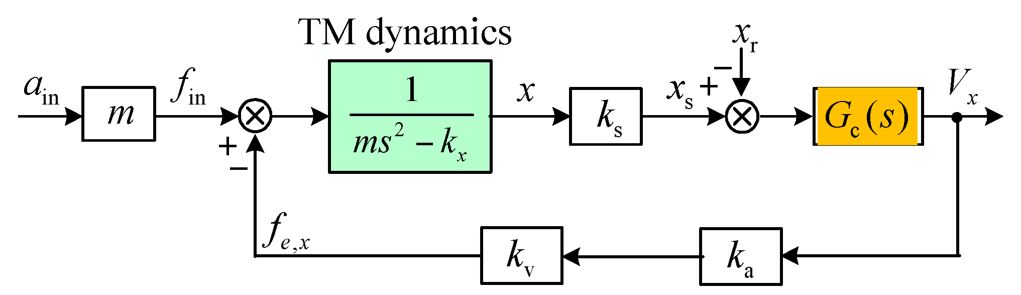
Open loop instability due to the negative position stiffness can be found by inspecting the characteristic equation of the transfer function in Equation (4) given the presence of a pole on the right-hand side of the s-plane. Consequently, active feedback control must be used to stabilize the suspension servo loop. A simplified block diagram of the closed-loop suspension control is shown in
Figure 6, where
,
and
are the sensitivity of the position sensor, gain of the voltage amplifier and transfer function of the feedback controller to be designed, respectively. It is assumed that no significant time delay (phase lag) occurs in the position sensor, digital controller and drive amplifier in the frequency range of the instrument operation.
For the NEP instrument operating in high vacuum, a typical lag-lead compensator is utilized to illustrate the design procedure:
where
is the compensator gain selected according to the stiffness requirements,
and
denote the time constants of the lag and lead compensators, respectively.
The closed-loop transfer function from the position reference input
to the position sensor output
is used as a measure of the loop dynamic performance and is given by:
Equation (6) describes the frequency response of the suspension servo to the position input. On other hand, the feedback control voltage is a measure of the acceleration input
ain applied to the instrument case. The transfer function that describes the accelerometer input-output response is defined as:
Equation (7) shows that the static and dynamic performance is closely related to design of the suspension control loop. At frequencies much lower than the suspension loop bandwidth, the TM is kept motionless in the electrode cavity due to high loop gain. In this case, Equation (7) can be simplified to a scale factor by considering that .
The electrostatic suspension loop is basically a regulator that keeps the TM centered at its equilibrium position. One of the most important characteristics of the accelerometer is the electrostatic stiffness provided by feedback control. The stiffness transfer function of the closed-loop system that relates the equivalent acceleration input force
to the position change
is derived from
Figure 6 and given by:
A fundamental controller design criteria for the suspension loop is to provide adequate stiffness and damping for stable suspension of the TM. The suspension stiffness is largely determined by the feedback controller within the loop bandwidth [
24]. Closed-loop suspension control must provide adequate positive stiffness, which is greater than the inherent negative position stiffness
to ensure loop stability. Hence, the suspension design must satisfy the following condition:
where
n is the ratio of the lowest overall stiffness to the negative stiffness of the TM and is usually
n ≥ 5 by design.
Given that the residual air-film effect in high vacuum can be neglected in design of the suspension loop, the lead compensation is utilized to provide adequate damping force and ensure desirable stability. The compensated open-loop transfer function in
Figure 6 can be given by:
It will be helpful to relate the lead compensator parameters in Equation (5) to the cross-over frequency of the open-loop system, e.g., let
. Substituting
s = j
ω into Equation (10), the cross-over frequency can be obtained by definition, i.e.,
:
where
n can be set by stiffness requirement and
b for desirable phase margin. The time constant of the lead compensator can be derived as
while the lag compensator usually has a time constant setting that satisfies
and
.
The design parameters of the
x,
y,
z-axis suspension are listed in
Table 4, where the
y/
z position stiffness also contains the contributions from the
x,
y,
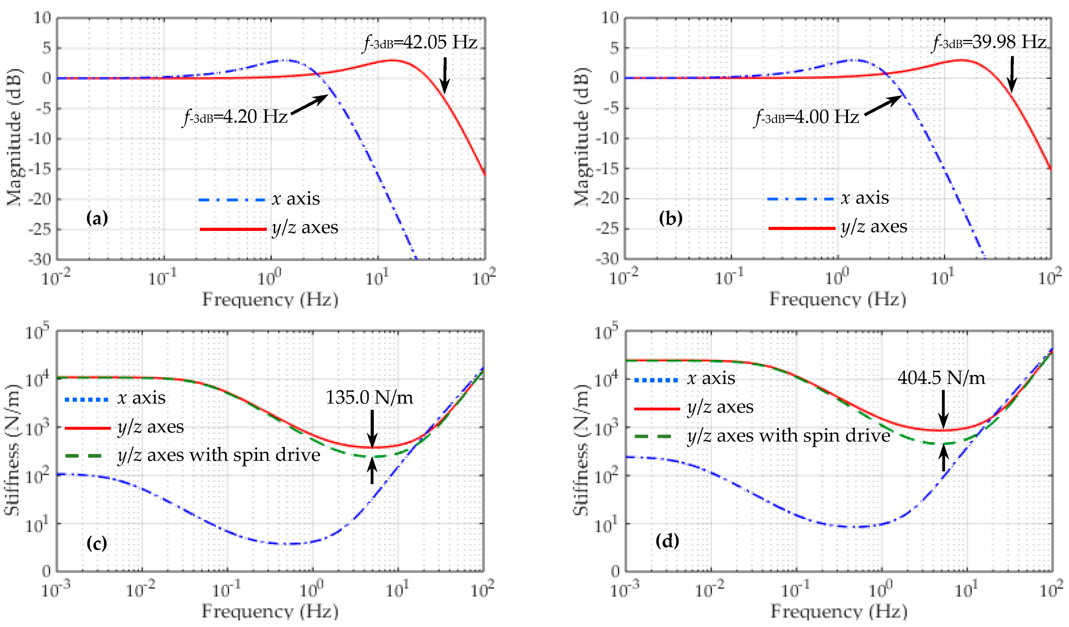
z-axis suspension electrodes and the injection electrode. The closed-loop frequency responses of the differential accelerometer operated in vacuum are simulated based on Equation (6). The simulation results of totally six closed-loop suspension loops, three for the inner TM and three for the outer TM, are shown in
Figure 7. It is clear that much different closed-loop bandwidths between the
x-axis and the
y/
z-axis suspension loops are shown in
Figure 7a,b. This result is attributed to the measuring range in the
y and
z axes of the inner/outer accelerometers being over 50 times larger than that in the sensitive
x axis.
Frequency responses of the suspension stiffness based on Equation (8) are shown in
Figure 7c,d. The simulated curves clearly indicate that these suspension loops have similar stiffness characteristics, except that the two radial (
y/
z) suspension loops have much higher stiffness than the axial (
x) loop in the low-frequency and medium-frequency ranges. On the other hand, these curves coincide closely in the high-frequency range (>200 Hz). This result can be explained by considering Equation (8) that each accelerometer has an identical inertial stiffness,
mω2. A design consideration in these suspension loops is that the stiffness characteristics must match the full-scale range of the accelerometer input. As an example, since the allowable input range in the radial direction is over 50 times larger than that in the sensitive
x direction, it can be observed that the radial suspension has extremely high stiffness compared with that of the axial suspension. At a frequency of 10
−3 Hz,
Figure 7 indicates that the
y/
z-axis stiffness is 100 times higher than that of the
x-axis suspension in our design. These results confirm the optimization of the instrument configuration for the
x axis as the measurement axis for the NEP test. The small full-scale range and low stiffness make it the most sensitive axis for the NEP measurements.
It seems that the closed-loop system exhibits relatively high suspension stiffness by setting a larger
n (
n = 15). For instance, the allowable displacement of the inner TM is less than 1.72 μm, only 2.87% of the nominal gap. However, the spin drive voltage during the electrostatic motor operation will also generate large unstable position stiffness [
25], e.g., 135.0 N/m by the inner motor and 404.5 N/m by the outer motor at a drive voltage of 100 V. In this case, the allowable motion range of the inner TM is increased to 2.67 μm but also well below the design goal of 10 μm. Considering that the unstable motor stiffness is over five times larger than the negative position stiffness
kx, its effect on the loop stability should be taken into account in design of the controller gain, as in Equation (9). In our design by setting
n = 15, the lowest closed-loop stiffness is over two times higher than the total negative spring constant, which ensures the loop stability even during the initial spin-up process.
3.3. Electrostatic Motor
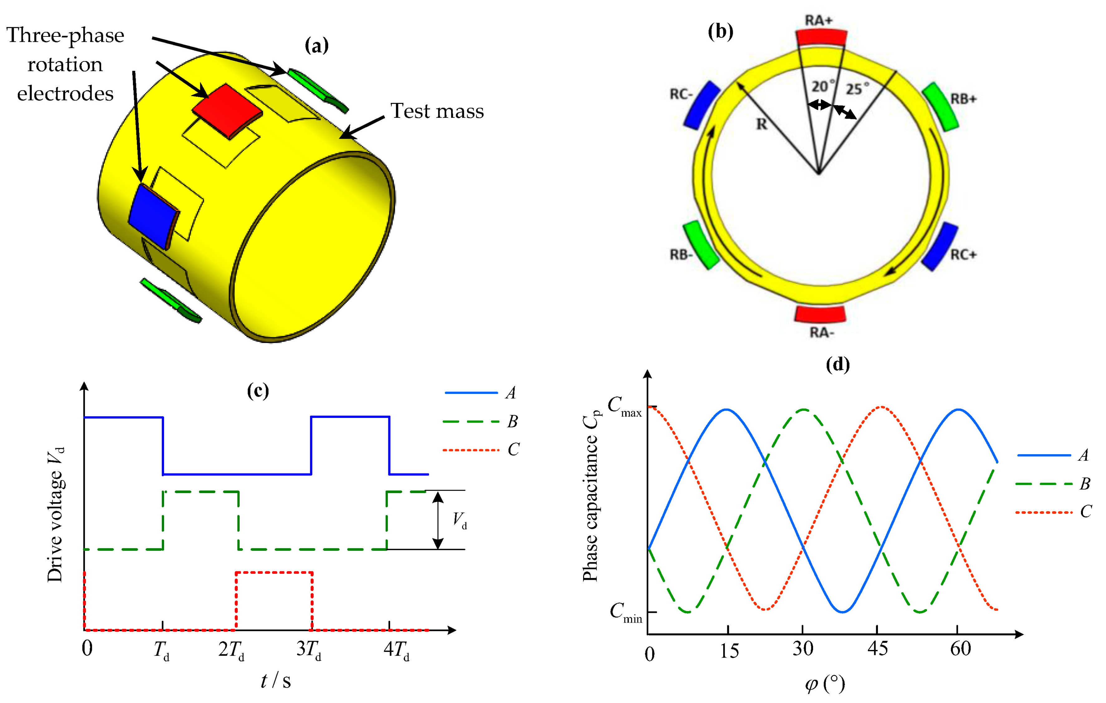
One important feature of the NEP instrument is that the two test masses are spinning with much different rotations. For this space accelerometer, each TM also features eight flat areas on its external surface as depicted in
Figure 8a, allowing the measurement and control of the axial mass spin. The rotation of the mass around the sensitive axis is measured though the differential capacitance change between the dedicated flat areas on the mass and associated rotation electrodes on the outer cylinder [
21]. The spinning-up of the mass is based on principle of the variable capacitance motor (VCM) consisting of a 6-pole stator (six rotation electrodes) and an 8-pole rotor (test mass). This VCM operates in a three-phase drive mode and produces a step angle of 15°, as shown in
Figure 8.
In order to simulate the steady-state speed and start-up time responses of the electrostatic motor, an analytical model governing the rotation behavior is necessary. For this three-phase VCM operated in high vacuum, the dynamic equation describing the TM rotation around the
x-axis can be expressed as:
where
and
are the axial moment of inertia of the mass and the damping coefficient generated by the residual gas in vacuum cavity, and
the drive torque produced by three-phase rotation electrodes.
Although the NEP instrument measurements are quite insensitive to the effects of electrostatic drive by comparing with classical electromagnetic motors, the drive torque produced by the electrostatic motor is extremely weak. Therefore, the start-up duration for a non-spinning mass to its rated speeds, 10
4 or 10
2 rpm in this work, will be quite long. Assuming the drive voltage is set at 100 V and the ultra-high vacuum reaches 10
−5 Pa,
Figure 9 shows the start-up time responses of the motor with different geometry parameters of the spinning TM. For instance, the start-up process from 0 to 10
4 rpm will last 1.657 × 10
4 s (4.603 h) for the inner mass and 3.452 × 10
4 s (9.588 h) for the outer mass, respectively. Fortunately, once the TM reaches its desired speed, the rotation drive will be switched off to avoid any possible disturbing forces produced by the rotation electrodes. Then the two TMs will be keeping free rotation virtually at their rated speeds. The small speed decay during each NEP experiment can be measured by a capacitive speed sensor and thus used to assist the NEP experiment data processing. Although longer time is needed to spin up the TM, the VCM drive is compatible with electrostatic suspension design and well suited for long-term space test of the NEP.
The NEP instrument can be set at several basic operation modes for calibration or NEP test, by considering that the two TMs can spin at various speed settings. When the two TMs are spinning at an equal speed, the instrument will be used as a reference to estimate various experimental limitations or systematic errors. On the other hand, in the NEP tests the two masses will be spinning at much different speeds, e.g., 104 rpm for the inner mass and 100 rpm for the outer mass and vice versa. Hence, unlike the STEP or MicroSCOPE mission enclosing two or more differential instruments made of different materials, the NEP tests can be performed using only one differential accelerometer with multiple rotation modes.
3.4. Noise Analysis
As stated in
Section 2, the desired acceleration noise along the sensitive axis is less than 2.0 × 10
−9 m/s
2/Hz
1/2 in order to test the NEP at a level of 10
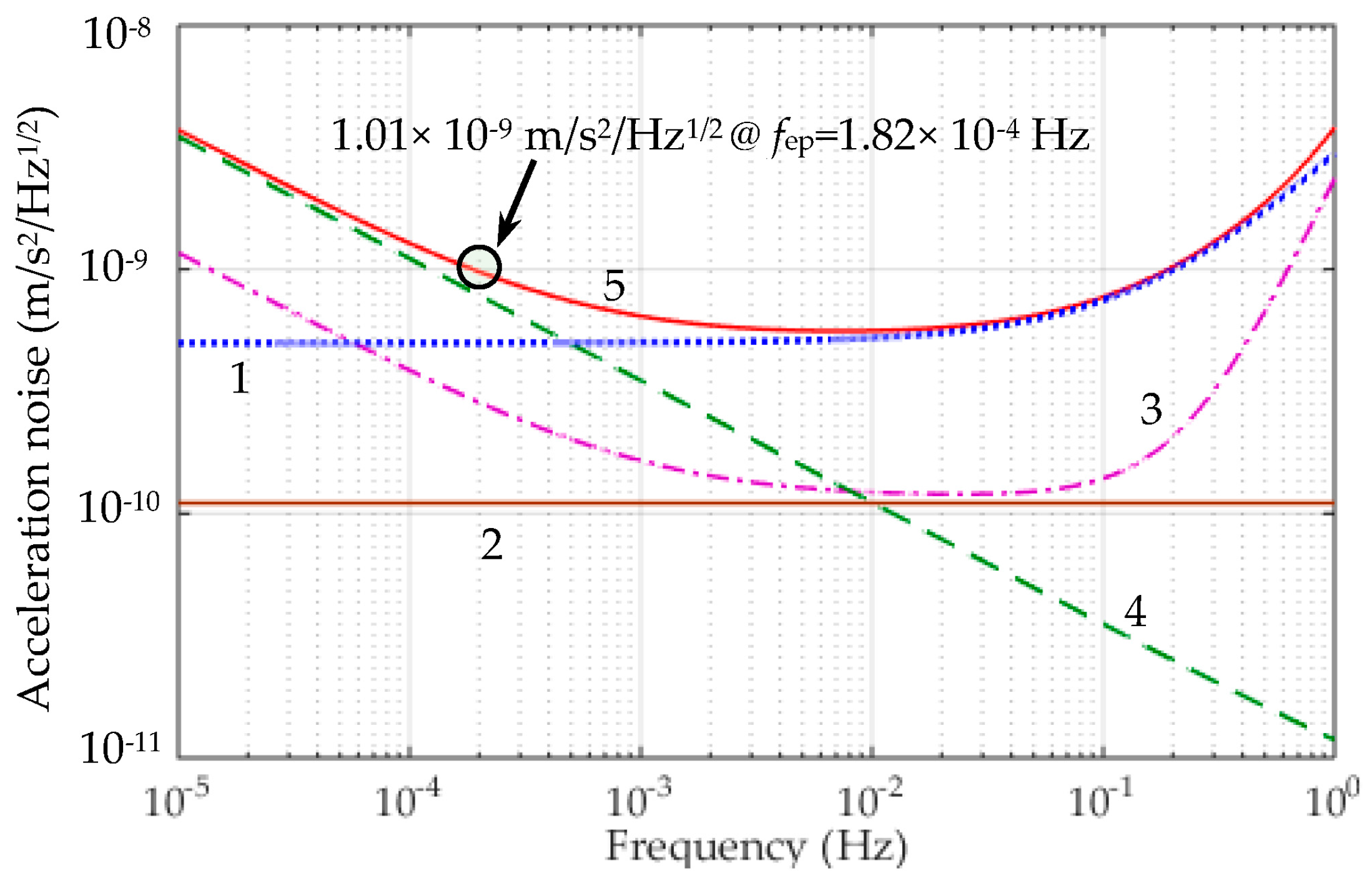
−12. The resolution of the NEP instrument is limited by various noise sources. The noise performance of the NEP instrument comprising of both the inner and outer accelerometers will be evaluated considering the following four major noise sources.
First, the differential acceleration between the TMs coupling from the residual non-gravitational acceleration
aec acting on the NEP experiment capsule can be written as:
where
Rcmr is the common mode rejection ratio of the differential accelerometer along the sensitive axis. In the NEP space tests, a drag-free control system with micro-Newtonian thrusters will be used to compensate for the non-gravitational forces acting on the experiment capsule, such as atmospheric drag force. It is estimated that the residual non-gravitational acceleration could be reduced down to 5 × 10
−6 × (1 +
f/0.1) m/s
2/Hz
1/2. According to the requirement of the MicroSCOPE mission, the
Rcmr could be realized to be 10
4. Thus the acceleration disturbance
ad is estimated to be lower than 5 × 10
−10 m/s
2/Hz
1/2, as shown by line 1 in
Figure 10.
Next, the thermal instability
δTd of the instrument core induces radiation pressure and radiometer effects due to the residual gas pressure
P inside the tight housing [
7]. The temperature effect including the thermal radiation pressure and radiometer acceleration can be expressed as:
where
σ,
c and
Am are the Stefan-Boltzmann constant, light speed and section area of the TM, respectively. Given the residual gas pressure
P = 10
−5 Pa, temperature
T = 300 K,
δTd = 0.5 K/Hz
1/2, the resulting acceleration disturbance for the inner and outer TMs are 1.27 × 10
−10 m/s
2/Hz
1/2 and 8.22 × 10
−11 m/s
2/Hz
1/2, respectively. The total temperature effect
atem is 1.51 × 10
−10 m/s
2/Hz
1/2, as shown by line 2 in
Figure 10.
At frequency range higher than 0.076 Hz, the position sensing noise
xnoise affects the acceleration resolution with a square frequency law, i.e.,
where
is the frequency associated to the residual passive stiffness
kx between the TM and associated suspension electrodes, which is evaluated to be less than 0.1 N/m by considering electrostatic field boundary effects. If the capacitive position sensor noise can be expressed as
xnoise = 4 × 10
−11 × (1 + 10
−3/
f)
1/2 m/Hz
1/2 [
26], the total acceleration noise
aPosition is less than 2.95 × 10
−10 m/s
2/Hz
1/2 at
fNEP, as shown in line 3 in
Figure 10.
At frequency range lower than 10
−3 Hz, the electrostatic actuation acceleration noise is the major source of noise and given by:
which depends mainly on the noise of the voltage amplifier
vnoise. In [
27], the voltage noise is estimated as
vnoise = 1.2 × 10
−8 ×
Vb × (1 + 7/
f)
1/2 V/Hz
1/2. Considering the actuator gain
kv and bias voltage
Vb in
Table 4, the voltage amplifier will contribute a total acceleration noise of 8.18 × 10
−10 m/s
2/Hz
1/2 at
fep, as shown in line 4 in
Figure 10.
Other accelerometer noise sources [
7], such as the thermal noise induced by the residual gas damping, coupling between the capsule’s attitude and the relative position of the two TMs, suspension induced electrical noise due to the spinning TM, the Earth’s gravity gradient effect and magnetic effect, have also been considered for the noise evaluation. These effects are in the range of over two orders of magnitude less than the NEP instrument noise goal, i.e., below 2 × 10
−11 m/s
2/Hz
1/2 at
fNEP. Thus these noise sources are negligible in the noise evaluation.
Taking the square root of the quadratic sum of four considered acceleration noises, the total differential acceleration noise is shown by line 5 in
Figure 10. The evaluated noise is 1.01 × 10
−9 m/s
2/Hz
1/2 at the NEP signal frequency, by neglecting other small acceleration disturbances. It is clear that the electrostatic actuation and residual non-gravitational acceleration are two major noise sources at the NEP signal frequency.


