The computing performance of the bundle adjustment method plays a relevant role in the development of a time-efficient in-process strategy for portable photogrammetry. The convergence time of the numerical method depends on the size of the Jabobian matrix , due to matrix element allocation, assignation and computation times for managing relatively large and sparse and matrices, and due to the conditioning and size of the inverse matrix calculation so that is determined in each iteration. As an example, given a measuring scenario with 100 images and 100 targets, assuming all targets are detected at every image, matrix size is 900 × 900, with being 40,000 × 900. Indeed, this problem increases with the number of images and targets included in the joint bundle during the measuring process. An alternative for reducing this computational work is the decomposition of the linear system to solve (Equation (8)) to a set of a lower range and individually solved linear subsystems. In this work, the reprojection error partial derivatives forming the Jacobian matrix (Equation (9)) are analytically expressed and system decomposition is adopted so that and are individually solved for interdependent extrinsic and target coordinate iteration, avoiding direct computation of in order to increase computational efficiency.
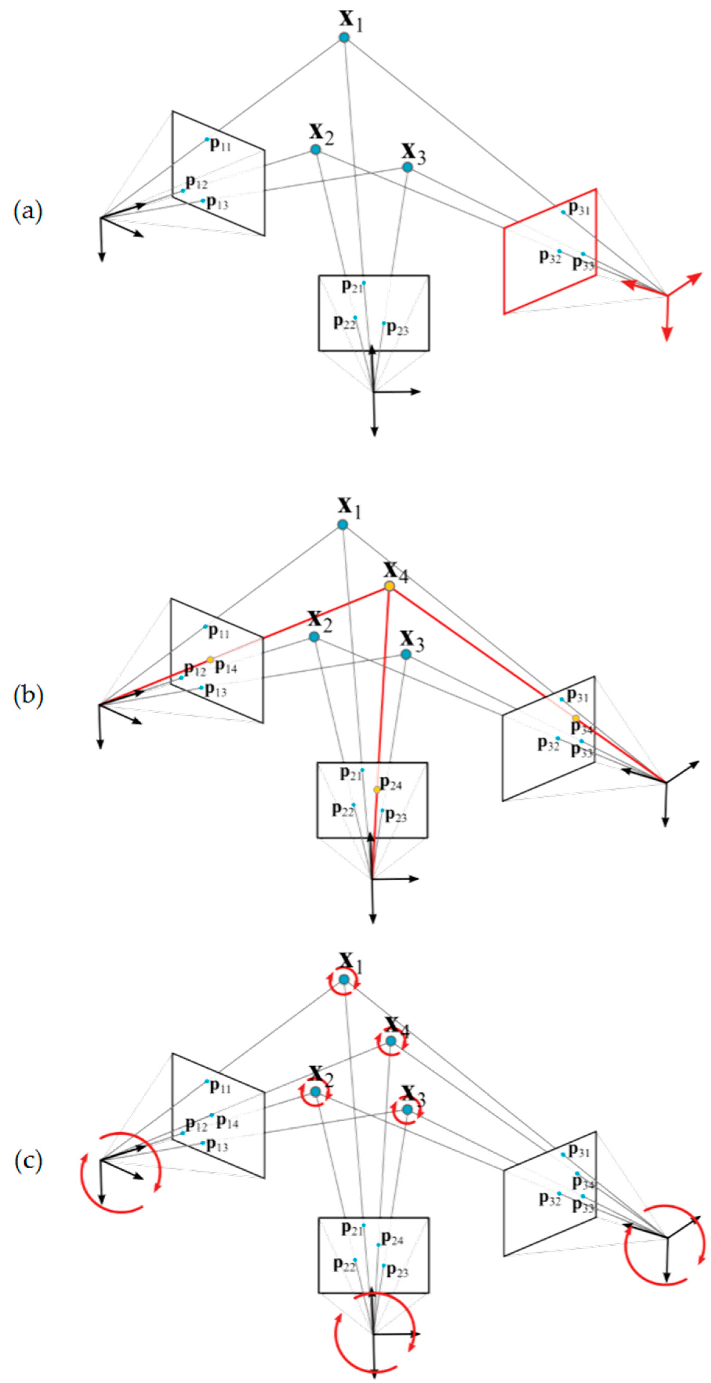
The main steps of the presented in-process strategy are described below. Results are shown for the pilot case under study (
Figure 3).
Section 4.1 and
Section 4.2 show the initial computation approach of the camera’s extrinsic parameters (step 2,
Figure 6a) and target coordinates (step 5,
Figure 6b) as independent computing problems, respectively.
Section 4.3 and
Section 4.4 describe the joint bundle adjustment problem both before (step 6,
Figure 6c) and after, including scale bars for traceability (step 7), respectively. Special attention is paid to the particular analytic expression of Equation (9) corresponding to each step of the in-process procedure. Although linear closed form expressions can be given in
Section 4.1 and
Section 4.2 for the independent camera extrinsic parameters and target coordinate computing [
24], nonlinear approaches are shown as intermediate steps towards presenting the submatrix decomposition of Equation (8) for the nonlinear joint bundle computation described in
Section 4.3 and the following. Optical target image coordinate detection (
,
) and decoding of coded targets is performed following [
29].
4.1. Camera Extrinsic Parameters Initial Approach Computation
Computation of the extrinsic parameters of a
j-th camera view (
Figure 6a) means determining vector
, where camera principal frame location (
,
, and
) and orientation (
,
, and
Euler angles defining a corresponding rotation matrix
as
) are defined with respect to a measuring frame (
Figure 4) determined by a pre-set of optical coded targets. The detection of a minimum set of 3 targets is required in order to geometrically determine image extrinsic computing.
As inputs for the method,
Xi coordinates of the set of coded reference targets are known, as well as camera intrinsic parameters (focal distance, and distortion model parameters for Equation (3)). As a result, partial derivatives (Equation (9)) in a Jacobian matrix
can be defined as follows (Equation (11)) for solving camera extrinsic parameters for the
j-th image as a nonlinear reprojection minimization problem.
where each submatrix
contains the partial derivatives of the projection errors
and
of the
i-th target
Xi coordinates with respect to the
j-th image camera extrinsic, to a total of
Nj optical targets detected in the that
j-th image. Each
submatrix can be expressed as
where
DP contains the partial derivatives of the
i-th projected target coordinates
and
in the
j-th image with respect to
target coordinates (Equation (1)) in the corresponding
j-th camera principal frame, given as follows according to Equation (2)
and where
expresses the partial derivatives of the
target coordinates with respect to the
j-th camera extrinsic in
as
given the partial derivatives
,
, and
of the camera principal frame rotation matrix
R with respect to each Euler angle
,
, and
, respectively.
At the beginning of the measuring process by portable photogrammetry, first images are taken to the set of coded targets determining the measuring frame. Given that a minimum number of three targets are detected in an image, the corresponding individual iteration of
and independent extrinsic computing can proceed for each image.
Figure 7 shows an example of computation of the extrinsic initial approach for the first three images of a measuring process conducted on the pilot case evaluation scenario (
Figure 3). Nominal values are adopted as an initial approach for the intrinsic parameters, with focal distance
f being 24.0 mm and first order radial distortion coefficient
being 5.0 × 10
−9 pixel
−2, where higher order radial distortion coefficients are neglected, along with decentering and tangential distortion coefficients in Equation (3). At this stage, the initial adopted approach for the intrinsic parameters is not intended to be accurate but only a nominal value close enough to the expected precise one, to be computed by the in-process self-calibration (see
Section 5) so that the final bundle converges in a stable and efficient way.
Table 1 presents the known 3D coordinates (
Xi,
i = 1 ..6) of the detected coded targets on each image, along with the detected image coordinates for each target at each image (
,
,
j = 1 .. 3).
Table 2 shows the computed extrinsic parameters for each camera view, according to Gauss-Newton method following Equation (8) for
iteration. The extrinsic computing performance can be observed in the resulting RMS value of the reprojection error vector after convergence, ranging at 0.5 pixels. Regarding computing efficiency, a mean time lower than 0.1 ms is observed for each iteration.
4.2. Target 3D Coordinate Initial Approach Computation
Once the camera extrinsic parameters are available (
Table 2), 3D coordinates of new targets other than those defining the measuring frame can be computed. Analog to extrinsic computing in
Section 4.1, the computation of the 3D coordinates of a
i-th new target (
Figure 6b) means determining vector
, where
Xi coordinates are defined in the same measuring frame at which camera extrinsic parameters are known. The detection of the target in a minimum set of 2 images is required in order to geometrically determine target coordinate computing by triangulation.
As inputs for the method, camera intrinsic and extrinsic parameters (
αj,
βj,
γj, and
dj) of a minimum set of images are known. As a result, partial derivatives (Equation (9)) in a Jacobian matrix
can be defined as follows (Equation (16)) for solving 3D coordinates for the
i-th target.
where each submatrix
contains the partial derivates of the projection errors
and
of the
i-th target with respect to its
Xi coordinates, to a total of
Mi images in which the
i-th target is detected. Each
submatrix can be expressed as
where
DP was defined in Equation (13), and
expresses the partial derivatives of the
target coordinates at the
j-th camera frame with respect to its
coordinates at the common measuring frame as
being
the rotation matrix corresponding to the
jth camera frame.
Following the example in
Section 4.1, given the computed extrinsic parameters of the set of three camera views (
Table 2), the iteration of
and the computation of the
Xi coordinates proceeds for coded targets detected at least in two camera views.
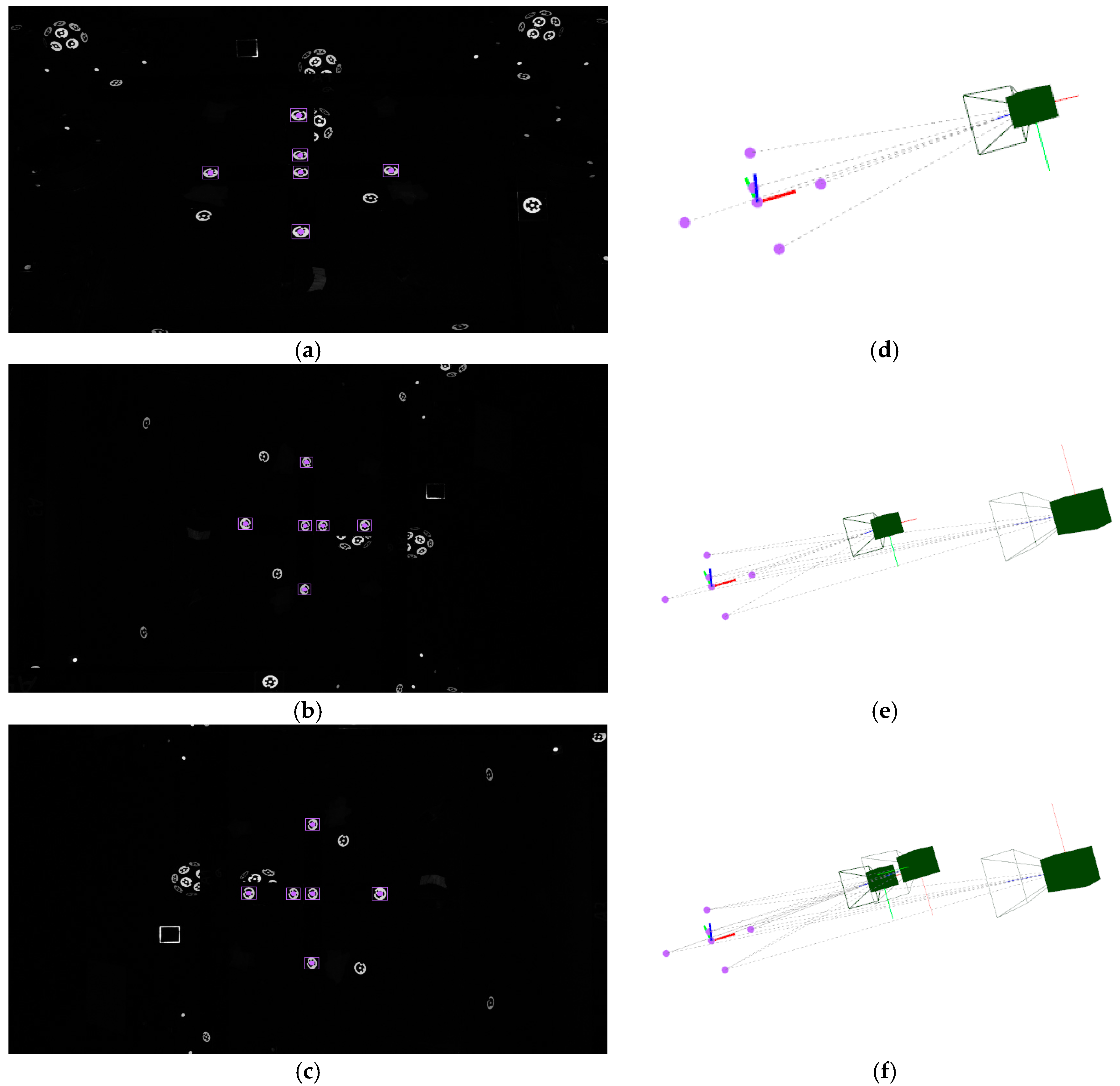
Figure 8 shows an example of computation of a coded target detected in all three images (
Figure 8a–c). Again, nominal values are adopted for the camera intrinsic parameters.
Figure 8d depicts the 3D location computed for that new target in the same measuring frame as camera views are given.
Along with computing the new target
Xi coordinates, new camera extrinsic parameters also enable code assignation to non-coded targets with pending correspondence to solve between detected coordinates in different images. The set of 3D epipolar lines given by the non-coded targets detected in all images can be expressed as 2D epipolar lines in each image. The distances from each 2D epipolar line to each non-coded target detected in the image can be calculated, so that the subset of 2D epipolar lines closest to a specific non-coded target in that image are likely to correspond to the epipolars of that 3D target detected in the other images. All possible 2D epipolar-to-target distances can be computed according to all possible correspondences between non-coded targets detected in three consecutive images, and the Hungarian method [
24,
29] can be adopted for solving the correspondences as the optimal combination which minimizes epipolar-to-target distance distribution among all 2D epipolars and non-coded target coordinates. As a result, codes can be assigned to non-coded targets in each image, and their 3D coordinate can be correspondingly computed.
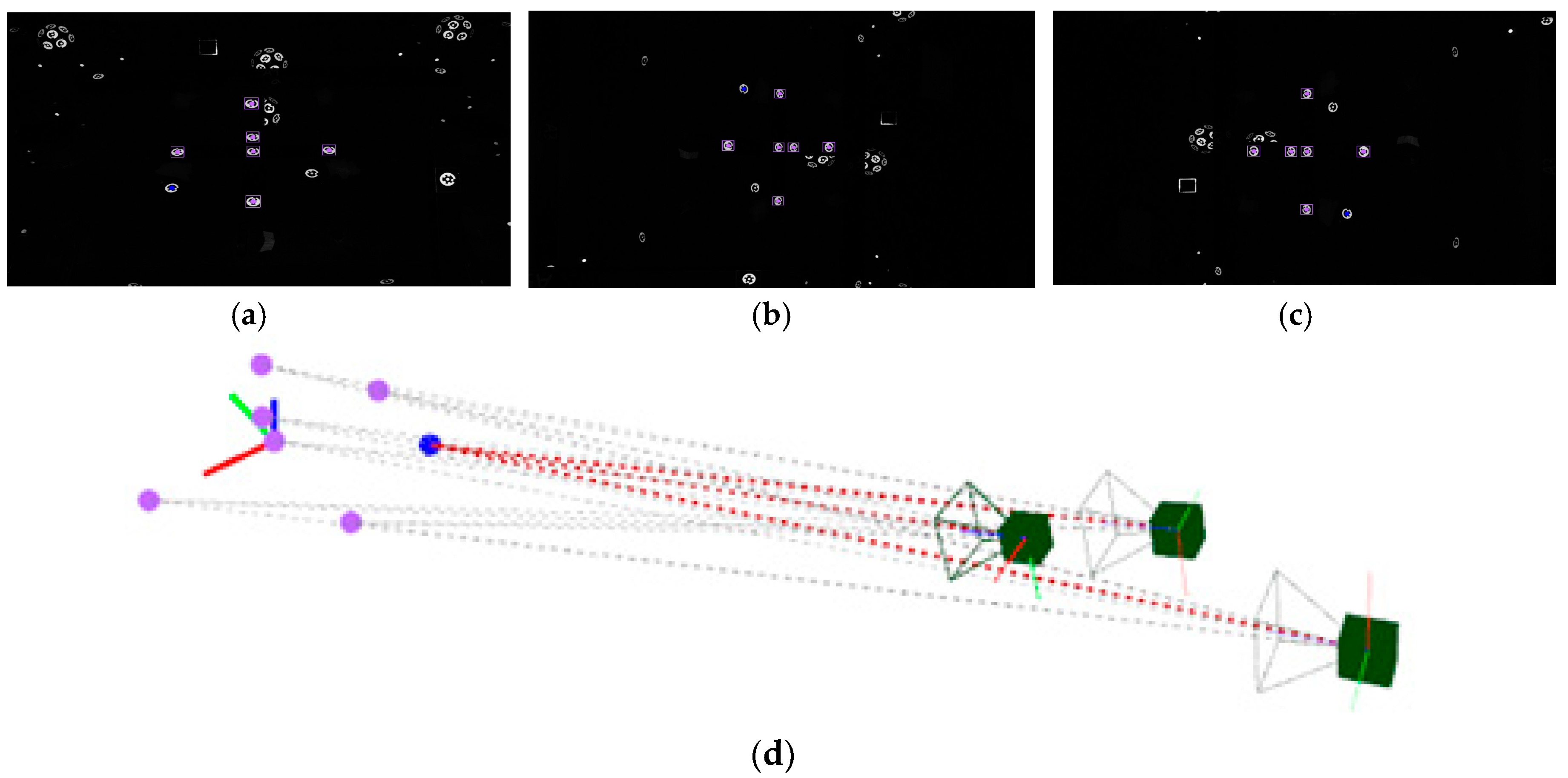
Figure 9a shows all the detected targets in the image presented in
Figure 8c, including both coded targets and non-coded targets with solved correspondences between the three images.
Figure 9b shows the resulting scene including the 3D coordinates of the computed new targets, along with the 3D epipolar net used to solve them. Computed target coordinates are listed in
Table 3, along with corresponding code identification and assignation (id) for coded and non-coded targets, respectively. The reprojection error minimization performance is also shown for computing each individual target, with a RMS value ranging from 0.085 pixels to 1.617 pixels. Again, the mean computing time ranges below 0.1 ms per iteration.
4.3. Joint Bundle Adjustment
Once the new target coordinates are solved, other than those defining the measuring frame, the bundle adjustment for joint computation (
in Equation (7)) of
i = 1 ..
N target 3D coordinates (
) and
j = 1 ..
M camera extrinsic parameters (
) proceeds, given by their interdependency through the epipolar net multiple view geometry (
Figure 6c). Now, partial derivatives (Equation (9)) in a Jacobian matrix
can be defined (Equation (19)) for minimizing a joint reprojection error vector of
2 m elements, being m as defined at the end of
Section 3.
with
and
containing the partial derivatives of each reprojection error with respect to all camera extrinsic (
αj,
βj,
γj, and
dj) and target coordinates (
Xi), respectively. Reprojection error vector elements can be arranged so that
can be defined as a non-square diagonal matrix with
submatrices in its diagonal with the partial derivative to each image extrinsic parameters
(Equation (11)) per the set of
Nj reprojection errors of all targets detected in each
j-th image, and
can be correspondingly expressed as a sparse matrix with
submatrices with partial derivative to each target coordinate
(Equation (17)) per the set of
Mi reprojection errors of each
ith target detected in its subset of images per
column and zeros in the rest of elements. Given this arrangement,
in Equation (8) can be expressed as follows
where
is a square diagonal matrix in which its diagonal is composed of
square submatrices accounting for each
j-th camera extrinsic contribution to the minimization problem in the least square sense, given
as defined in Equation (11), and
is also a square diagonal matrix in which its diagonal is composed of
square submatrices accounting for the contribution of the 3D coordinate of each corresponding
i-th target detected in its
Mi image subtset, given
as defined in Equation (17).
is a non-square sparse matrix where the interdependency between extrinsic parameters and target coordinate computation through the joint epipolar net is taken into account, with elements contributing along with the joint product of the partial derivatives to image extrinsic and target coordinates for a i-th target detected in a j-th image, and zero when a i-th target is not seen in a j-th image, given as defined in Equation (12).
Thus, according to Equation (20), Equation (8) can be decomposed as
where the residual term
can be redefined according to Equation (19) as
Given Equations (21) and (22), the linear system in Equation (8) can now be decomposed to a set of two lower range subsystems where
and
can be individually solved for interdependent extrinsic and target coordinate iteration, where extrinsic iteration
can be obtained as
and target coordinate iteration
can correspondingly be given as
Following the examples in
Section 4.1 and
Section 4.2, given the computed initial approaches for the three first image extrinsic parameters (
Table 2) and for the corresponding target coordinates (
Table 3) in the evaluation scene shown in
Figure 9b, their joint computation can be conducted according to Equations (23) and (24). As inputs for the method, 3D coordinates of the set of coded targets on the measuring frame are known (
Table 1), as well as nominal camera intrinsic parameters, along with image coordinates of coded and non-coded target with solved correspondences between images (
Table 1 and
Table 3).
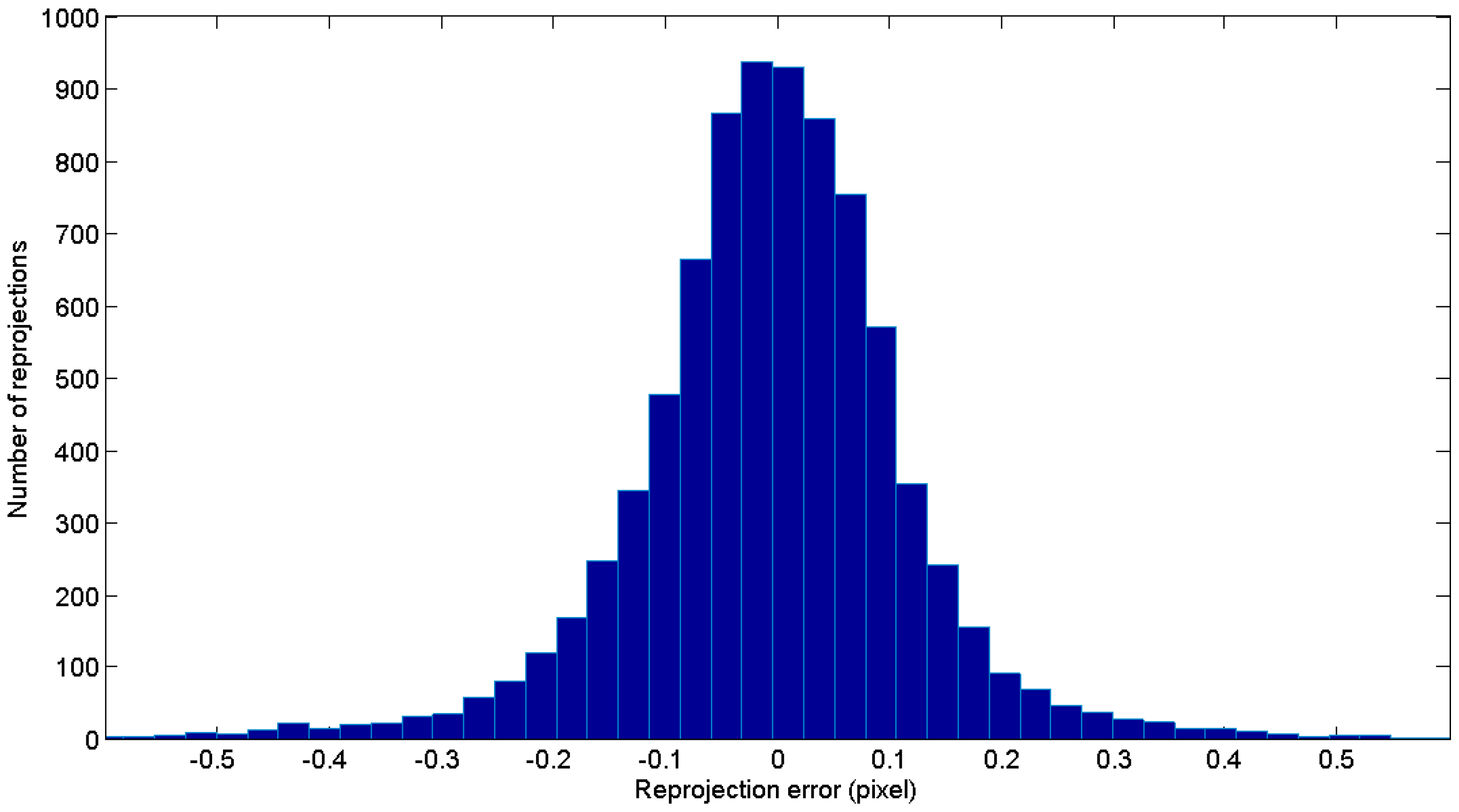
Table 4 and
Table 5 show the results of the intermediate joint bundle computing for extrinsic parameters and targets (step 6 of the in-process procedure), respectively. The RMS of the joint reprojection error is optimized to 0.802 pixel, with an iteration time of 0.17 ms.
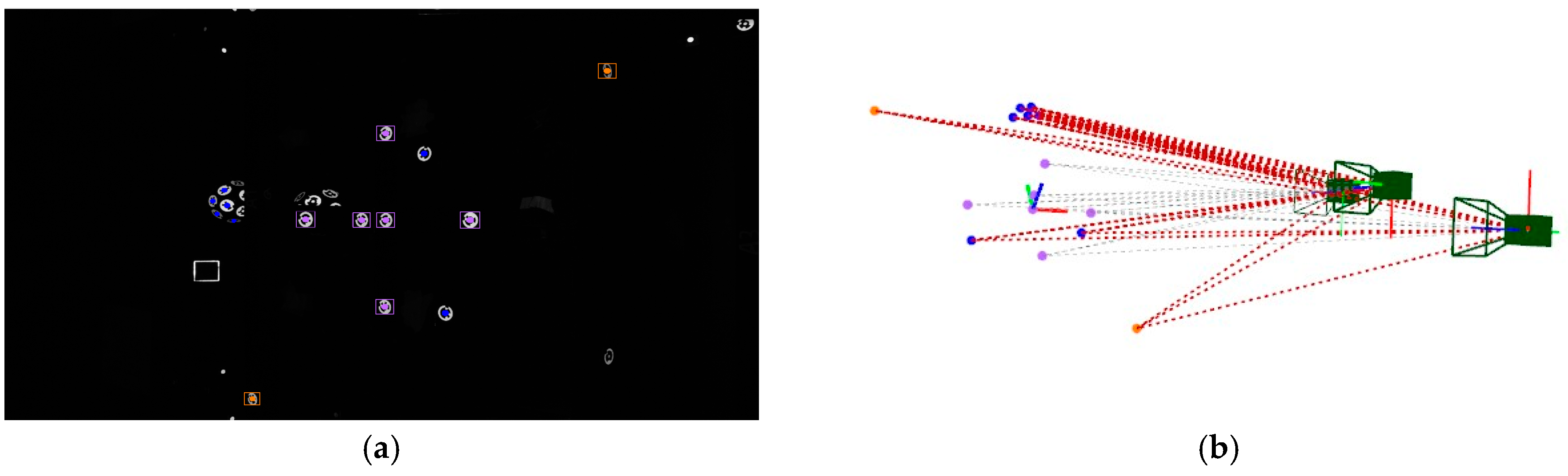
The measuring process may now continue with the acquisition and in-process computing of new images, following the in-process procedure described in the introduction of
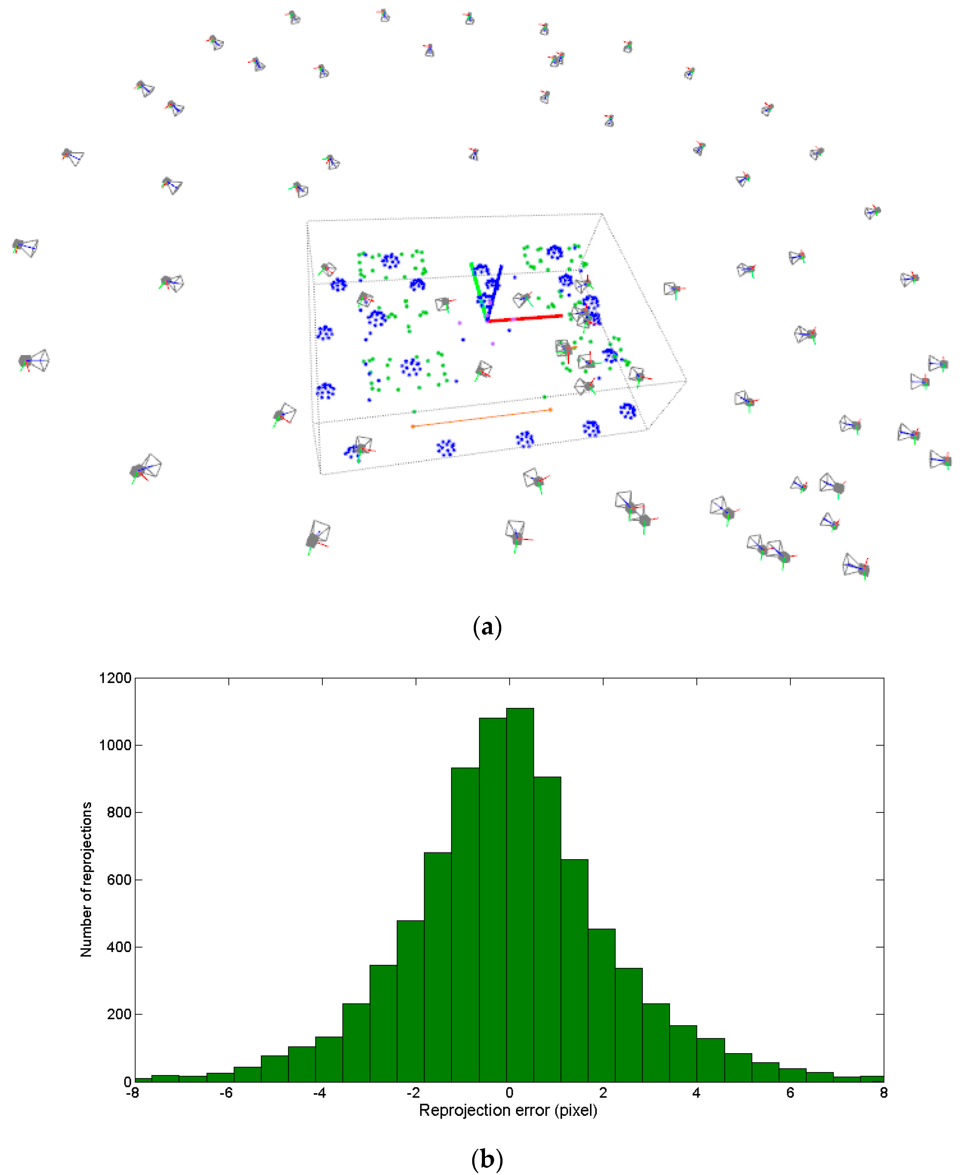
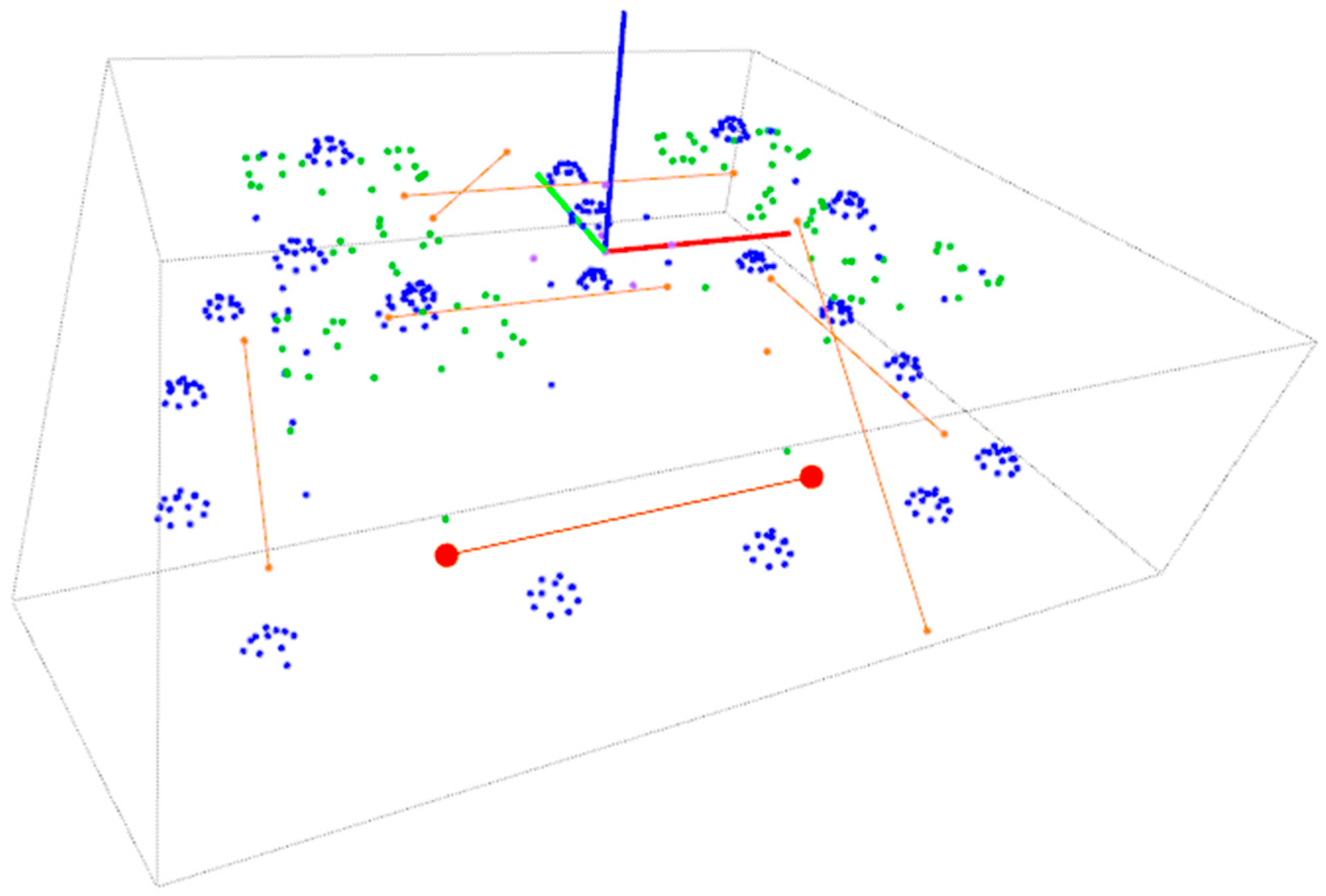
Section 4 (steps 1 to 6). An example of a complete measuring set is shown in
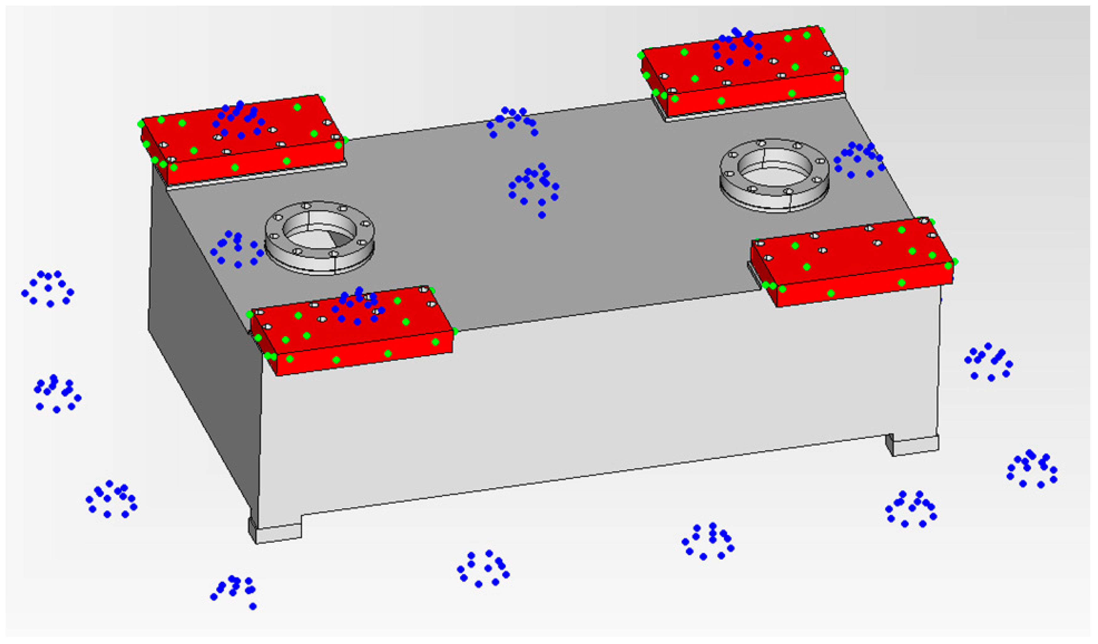
Figure 10a for the pilot case under study (
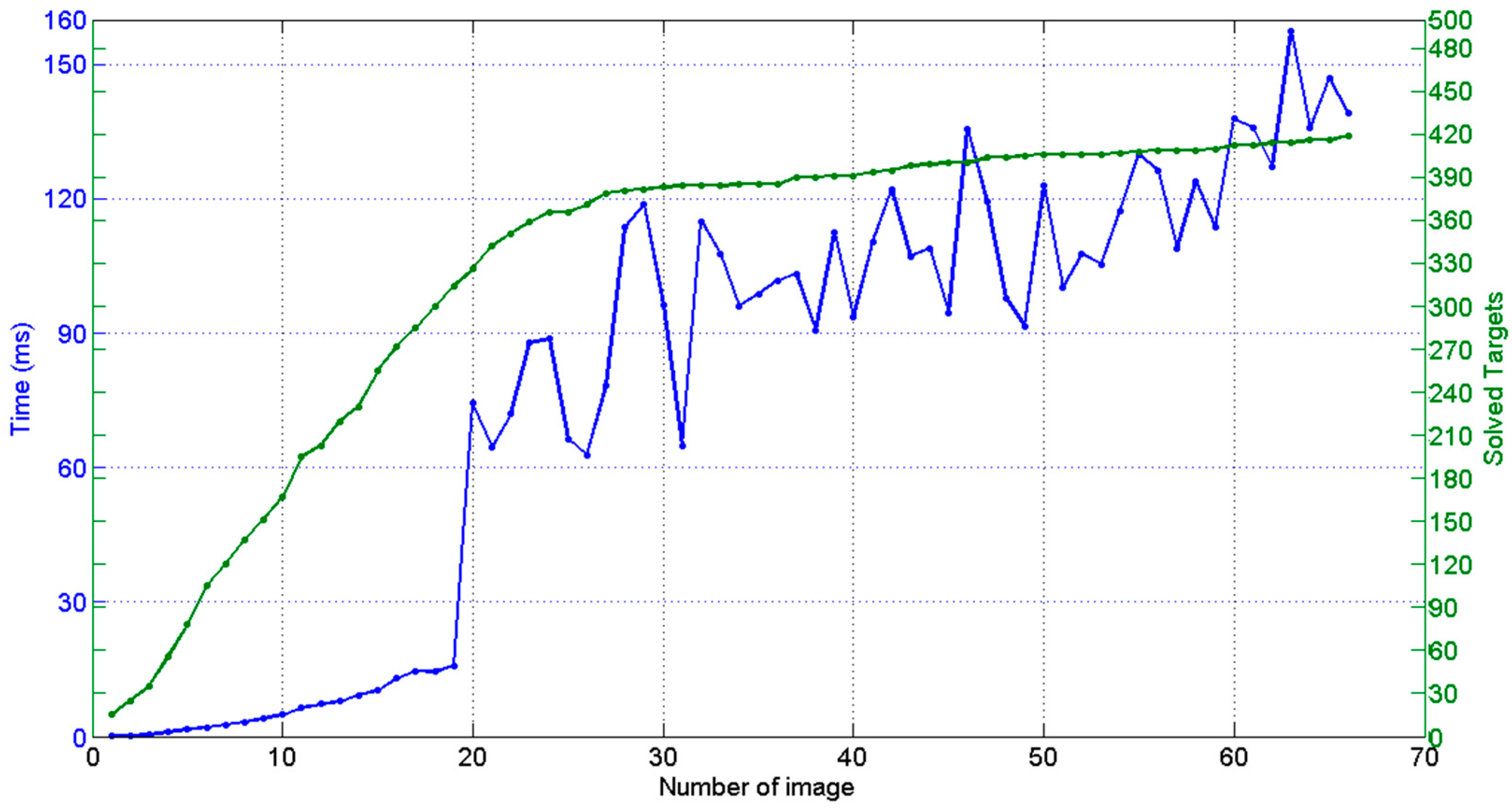
Figure 3), where non-coded targets were placed on the milled surfaces and coded targets were placed around the scene enabling a consistent epipolar net construction during measurement, along with the reference frame with its corresponding coded targets. A total number of 68 images were taken, solving the 3D coordinates of 80 non-coded (20 at each milled prism) and 340 coded targets. A maximum joint bundle computation time ranging 150 ms was observed for the last images of the measuring process (see
Section 4.4).
So far, the measuring scale and traceability depend on the coded target 3D coordinates defining the reference frame (
Table 1), along with the adopted nominal camera intrinsic parameters. An alternative for increasing accuracy in portable photogrammetry is the adoption of appropriate scale bars with calibrated lengths between corresponding pairs of optical targets (highlighted in orange in
Figure 10a), so that measuring process traceability is given by precise scale bar distances. Then, once image-taking finishes (steps 1 to 6), the final post-process joint bundle of camera extrinsic parameters and target coordinates can proceed until convergence (step 7), imposing calibrated relative distances between corresponding pairs of target coordinates in each scale bar available in the scene. A free network adjustment is then carried out. For this, the 3D coordinates of the coded targets on the reference frame (
Table 1) have to be also computed, so that their assumed coordinates so far (in steps 1 to 6) do not influence measuring process traceability, and the measuring frame is correspondingly redefined according to their computed coordinates following the widely adopted 3 (to define a reference plane) −2 (to define a reference axis) −1 (to define the origin point) rule in metrology, setting back a determined origin and orientation to the measuring coordinate system.
To do so, a corresponding error vector
can be expressed (Equation (25)) and its corresponding joint minimization can be accomplished along with the reprojection error vector
in Equation (4).
where
expresses (Equation (26)) the square distance between each pair of target coordinates minus the corresponding scale square length, given by
, from
k = 1 ..B bars with
scales in the scene, with
and
being the 3D computed coordinates for each pair of targets of the
kth scale bar, which can be expressed as
and
contains (Equation (27)) the 3D coordinate errors of a set of reference targets selected for determining the measuring coordinate system according to the 3-2-1 rule, which can be expressed as
where a first reference target
X0 is set and constrained to be the coordinate system origin (X
1 in
Table 1), so that
coordinates have to be minimized to zero as first elements in
setting 3 restrictions, a second reference target X
1 is constrained (X
3 in
Table 1) to have its
Y and
Z coordinates to zero, so that
and
coordinates in
are included as the next elements in
setting 2 restrictions determining
X coordinate axis, and a last reference target
X2 is constrained (
X4 in
Table 1) to have its
Z coordinate to zero, so that
coordinate in
is included as the last elements in
setting 1 restriction determining
XY plane of the measuring frame. As a result, 6 constraints are included and a coordinate system is determined, the rest of the initially assumed reference target coordinates (
Table 1) being unconstrained and correspondingly computed, so that measuring traceability is now set by the scales imposed in Equation (26).
A Jacobian matrix
corresponding to
minimization problem (as in Equation (8)) can be defined as follows
where
contains (Equation (29)) the partial derivatives of the
k = 1 ..
B square distance errors to the each pair of corresponding target coordinates
and
given as
being each
with derivatives
and
following Equations (31) and (32) and zeros for the rest of the elements in
, being
N the new total number of computed targets,
and
expresses the partial derivatives of
to the constrained reference target coordinates, equal to 1 at the columns corresponding to each computed coordinate, and zeros in the rest of the elements.
Thus, a joint error vector
can be defined as follows (Equation (33)) integrating reprojection errors in
along with error vector
and joint bundle can be conducted (as in Equation (8)) with the corresponding redefined joint Jacobian for numerical iteration as
Following the same system decomposition approach as in Equations (21)–(24), it can be demonstrated that the main iteration equations given by Equation (21) can be redefined to a similar form as
where terms
and
are redefined to
and
according to
and
as
so that expressions given at Equations (23) and (24) for
and
, respectively, can be used for computing to convergence the post-process joint bundle (step 7) of the scene extrinsic and target coordinates integrating scale and 3-2-1 rule restrictions. As input for the post-process joint bundle, results after processing the last image at step 6 are known.
Figure 10b shows the corresponding histogram of the minimized reprojection error vector
after joint bundle with
, resulting in a RMS value of 2.378 pixel.
4.4. Computing Performance of the In-Process Approach
The procedure described above was developed in C++ language, using the OpenCV library for image processing and the Eigen library for matrix management and processing, on a desktop PC Intel Core i7-5600U 2.6 Ghz, with 16 Gb RAM, running on Windows 7 with 64 bits. Wireless image transmission was used, observing a transmission time of 0.5–1 s per image for 12.2 Mpixel raw images. Image processing time (step 1) was observed to reach 0.5 s per image, depending on the number of segmented and decoded targets on the image. Computing time for the initial extrinsic and target approach (steps 2 and 5) for new images and targets prior to their first bundle could be relatively neglected, ranging below 1 ms. Code assignation to non-coded targets (step 4) was observed to range up to 0.1–0.3 s per image, depending on the number of non-coded targets and correspondences to solve between images.
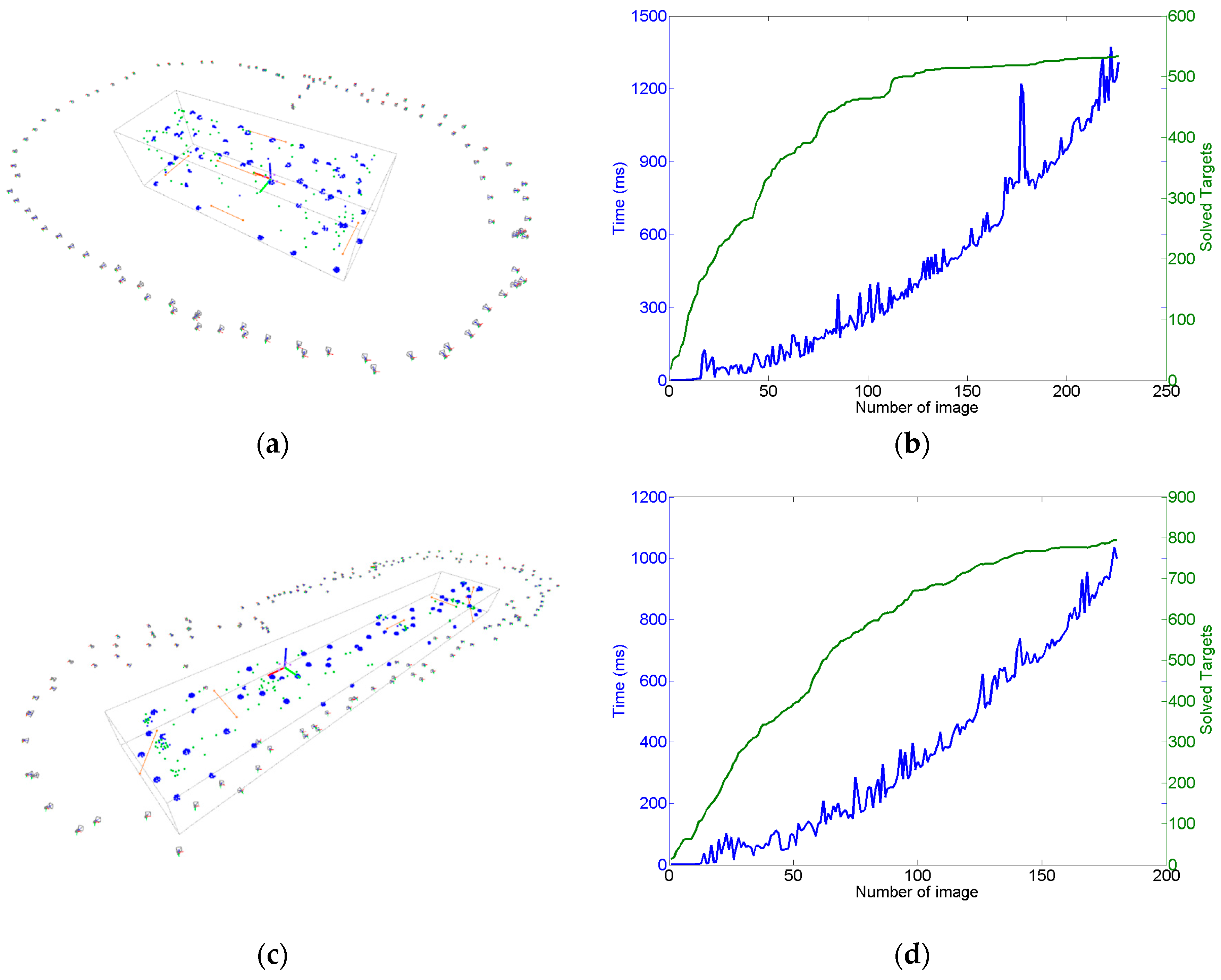
Figure 11 shows the dependence of the computation time of the intermediate bundle (step 6) on the number of cumulated images and solved targets so far during the measuring process, with a time ranging up to 0.15 s per image for the last images of the measuring scenario shown in
Figure 10. As a result, total in-process computation time (steps 1 to 6) ranged at a maximum of 1 s per image, in the same order of magnitude of the wireless image transmission time itself.
However, an average increase of 3 ms per additional image can be estimated from
Figure 11 for step 6, which would lead to relevant in-process computation time contribution if larger measuring scenarios were adopted with more images and targets. If a better in-process computing performance was required for step 6, further optimization could be conducted following the system decomposition approach presented in this paper, taking advantage of the symmetry and characteristics of the involved submatrices in Equation (21) (diagonal A and C submatrices, dominating presence of zeros in sparse B submatrix, etc.) along with the development of analytic expressions for the involved inverse matrices in Equations (23) and (24).
Finally, the post-process joint computation time (step 7) reached 3 s in the same scenario, with 5 iterations to convergence, assuming convergence criteria of and being below a minimum iteration value of 10−6 mm and 10−6 radians for all location and orientations, respectively.

 and
and 


