1. Introduction
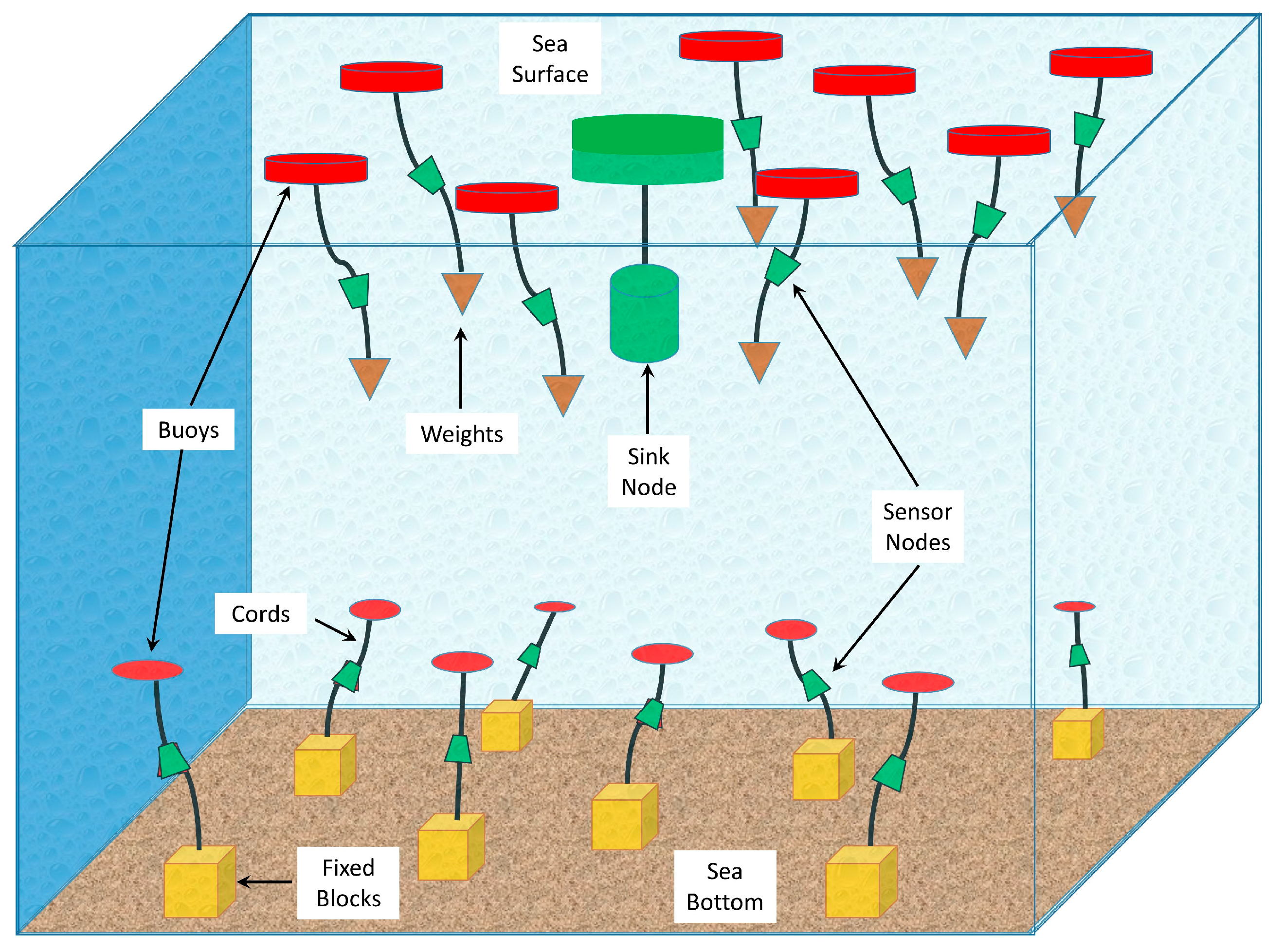
Underwater wireless sensor networks (UWSNs) have many applications related to environmental monitoring, disaster alerts, and military surveillance. UWSN may be deployed in either shallow or deep waters. When a sensor network is deployed in shallow waters and sensors are attached to the bottom of the sea, a 2D deployment of the network is considered. In deep waters, the nodes are suspended by a rope or a chain, which is attached to the surface buoys or the anchors at the bottom of the sea (
Figure 1). The suspended sensor nodes in 3D networks keep moving in all directions. This movement is limited by the length of the connecting rope or chain. The continuous random movement of the nodes makes the protocols design more challenging in 3D networks.
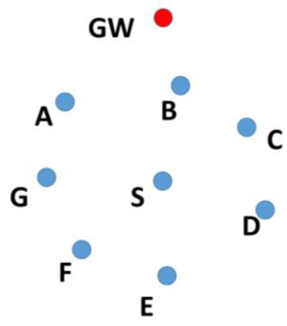
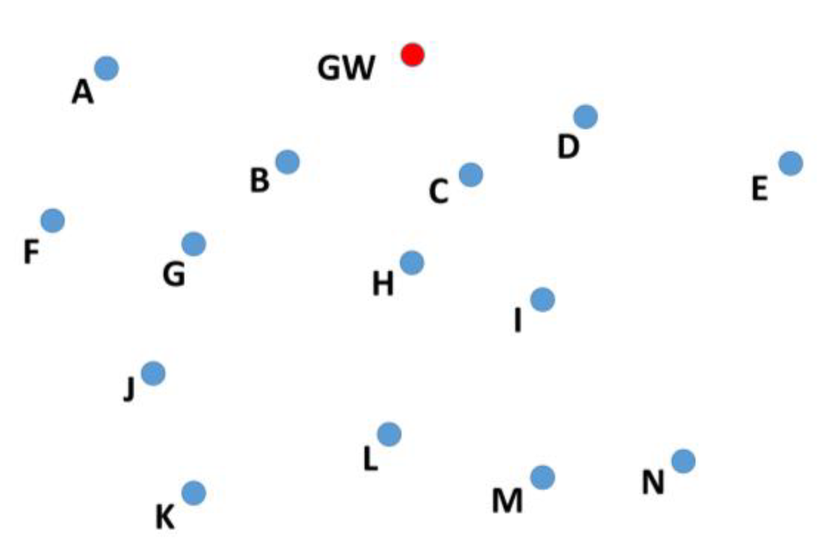
In a cooperative network, the nodes farther away from the sink node, also known as the gateway (GW) node, send their data to the GW with the help of intermediate nodes known as relay nodes. To select a relay node, the position of its candidate nodes should be known. For example, nodes A, B, C, D, E, F, and G in
Figure 2 are at one hop distance from node S. All of these nodes will receive the data transmitted by node S, but only the nodes closer to the GW should retransmit the data. Therefore, before node S can select one of these nodes, it needs to know the position of nodes A, B, C, D, E, F, and G.
In WSNs, determining the location of a sensor node is trivial. The sensor nodes can directly determine their position with the help of Global Navigation Satellite Systems (GNSS). However, this process in UWSNs is a challenging task because the GNSS signal is not present. One way to determine the position of the underwater nodes is that the GW gets its position with help of GNSS and the rest of the nodes determine their position with respect to the GW. However, in a 3D network, it is very difficult to determine their position by this method because of the continuous limited movement of the nodes.
In UWSNs, the position of the nodes can also be determined by Time Difference of Arrival (TDoA) [
1] and Time of Arrival (ToA) [
1]. TDoA is based on the two different transmission-media, like radio frequency and acoustic wave. The distance is estimated by different arrival times due to the dissimilar velocities of the radio wave and acoustic wave [
2]. However, EM waves are not available and TDoA cannot be used in underwater environments. The time of Arrival (ToA) technique is an alternative approach; it is based on the travel time of the acoustic wave from the source to the destination. The sender stamps the time of sending the packet and the receiver calculates the travel time by comparison to its local time and estimates the distance. This method requires time synchronization between the sender and the receiver nodes. Achieving time synchronization among the nodes in a UWSN is very difficult because of variance in the acoustic waves’ propagation speed and limited mobility of the sensor nodes caused by the water currents.
As an alternative method, the position of the nodes can be determined by measuring their distance from the water surface by means of depth sensors. This method is used by many routing protocols, like DBR [
3], LB-AGR [
4], and VBF [
5]. However, depth sensors have their own disadvantages, like measurement errors, increase in power consumption due to depth sensing and computation, and the extra cost [
6].
Because of the constraints and disadvantages mentioned above, the routing protocols which are based on neither the location of the sensor nodes or use the depth sensors are more practical and beneficial. In this paper, we use the distance between the sender node and the candidate nodes as a metric of selection for the relay node, estimated by the received signal strength (RSS).
After a review of the state of the art of underwater routing protocols in next section, the three metrics used in the new protocol proposed are explained in detail (
Section 3). Later on, the process to build the routes is examined (
Section 4) and a mathematical analysis is performed (
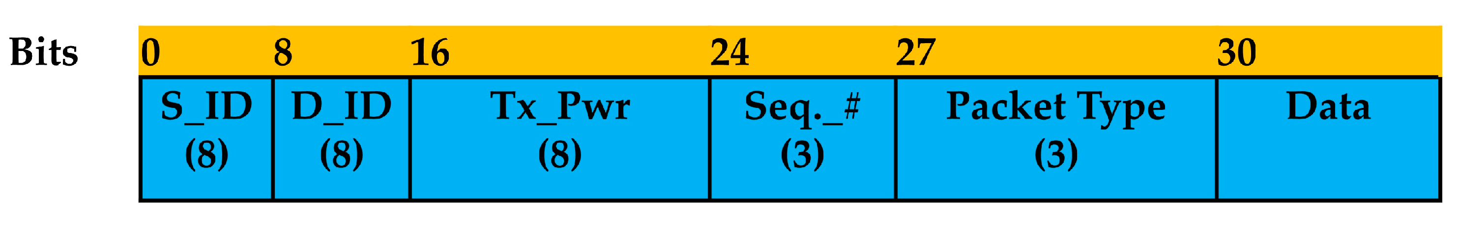
Section 5). Next, a suitable packet format is stablished in
Section 6, and results of simulations are presented (
Section 7) with a discussion of their importance. Finally, the final conclusions are remarked.
3. Overview of the SPRINT Protocol
The RSS metric is used to estimate which node is the closest neighbor of the transmitting node. The node selects the node that is closest to it to forward the packet. Along with the distance, two more metrics are used: number of hops between the sender and the sink, and the number of neighbors of the candidate nodes. The minimum distance between the nodes also increases the probability of successful packet delivery.
The estimation of the RSS is not very precise due to the path loss, the fading, and the limited mobility of the sensor nodes. The spreading of acoustic signal is an important factor for path loss. Spreading losses depend not only on the transmission range, but also on the propagation model adopted: cylindrical (shallow waters) or spherical (deep waters). The path loss is also due to absorption. The absorption of acoustic channels depends on the frequency of the acoustic signal. Total path loss
[
19] due to spreading and absorption can be expressed in decibels by the following equation:
where
(km) is the transmission range of the acoustic signal,
is the spreading factor,
(in dB/km) is the absorption coefficient, and
(kHz) is the frequency. The value of
is for cylindrical spreading, and
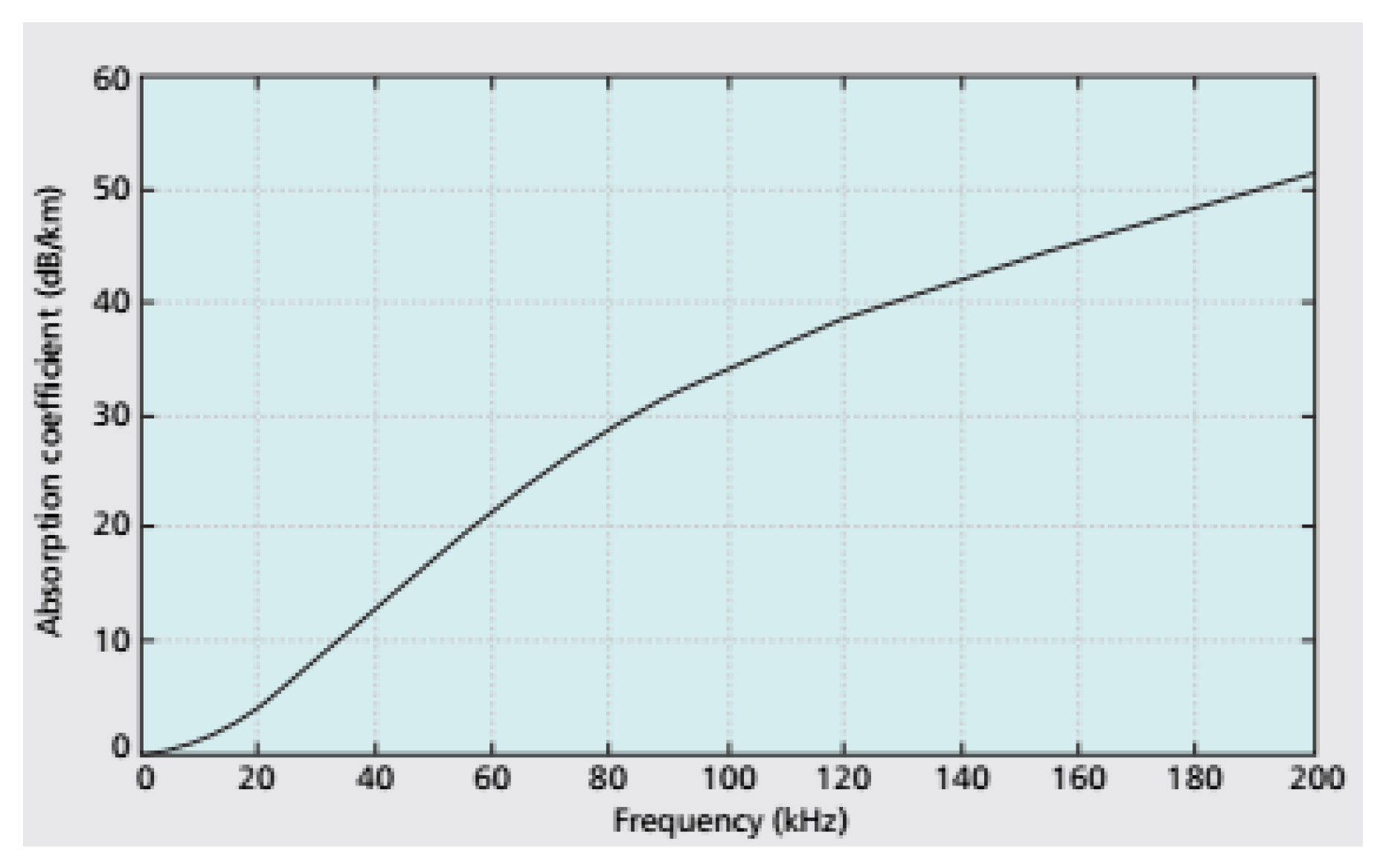
for spherical spreading. A graph of absorption coefficient versus acoustic signal frequency is depicted in
Figure 3 [
20]. We can see that for frequencies up to 20 kHz,
is <4 dB/km (approximately).
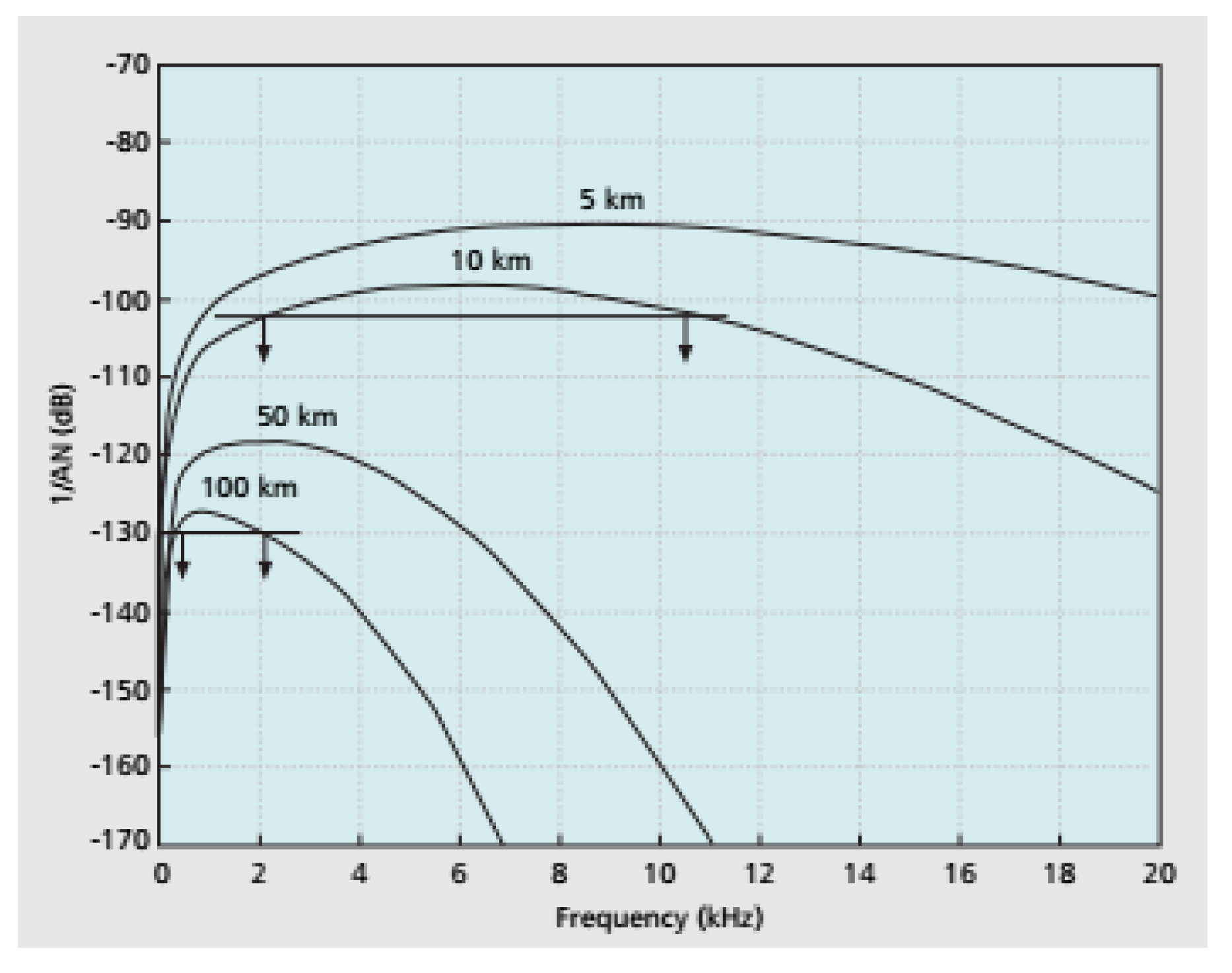
Figure 4 [
20] shows that Signal-to-noise ratio (SNR) also depends on the frequency. This figure also shows that the bandwidth of acoustic signal depends on the distance. For 100 km, the bandwidth is about 1 kHz, whereas for 5 km it is about 10 kHz.
Fading is more severe in shallow water compared to deep water due to multipath. There are no standard fading models for acoustic communication, and experimental measurements are used to predict the channel behavior [
20]. For this protocol, the error in estimation of RSS due to losses, fading, and limited mobility of the nodes is not significant as long as a node successfully forms a path with one of its neighbors that is closer to the gateway. The error in node selection may be corrected later by measuring the RSS value at regular intervals using the data packets.
Our proposed protocol assumes that the nodes are deployed randomly in a 3D network. The minimum distance between nodes is 300 m and maximum is 1000 m. The transmission power is adaptable and can be adjusted according to the distance between the transmitter and sender. The nodes are not stationary and keep moving in all directions, although their movement is limited by the length of the binding lines to the surface buoy or the anchor at the sea bottom (see
Figure 1). Lists of the acronyms and symbols used in this paper are shown in
Table 1 and
Table 2, respectively.
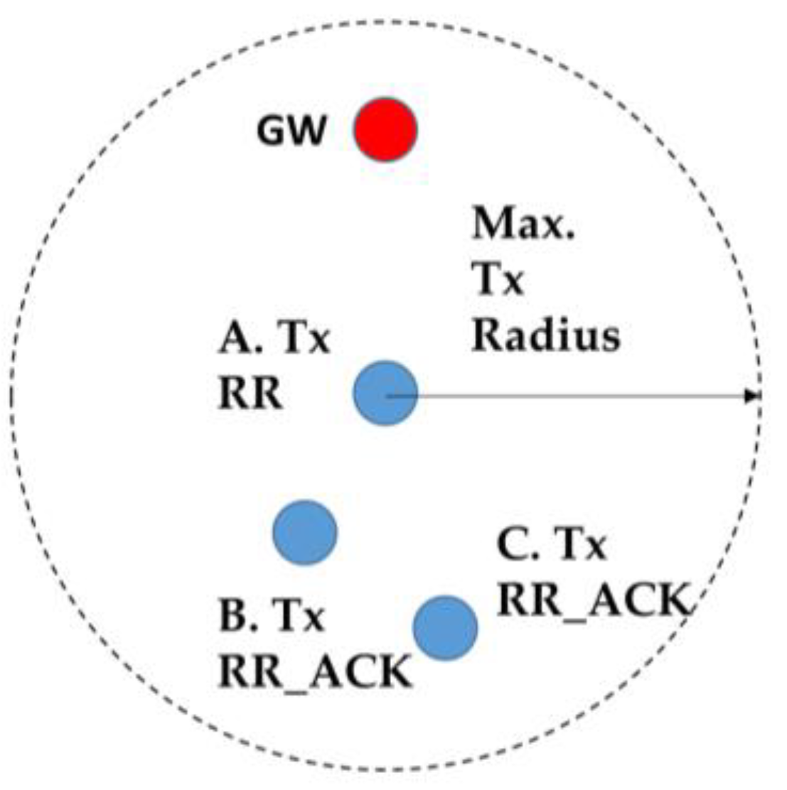
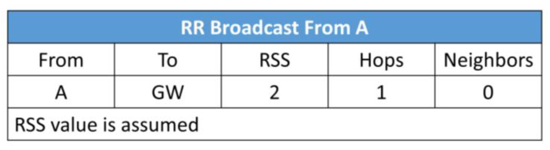
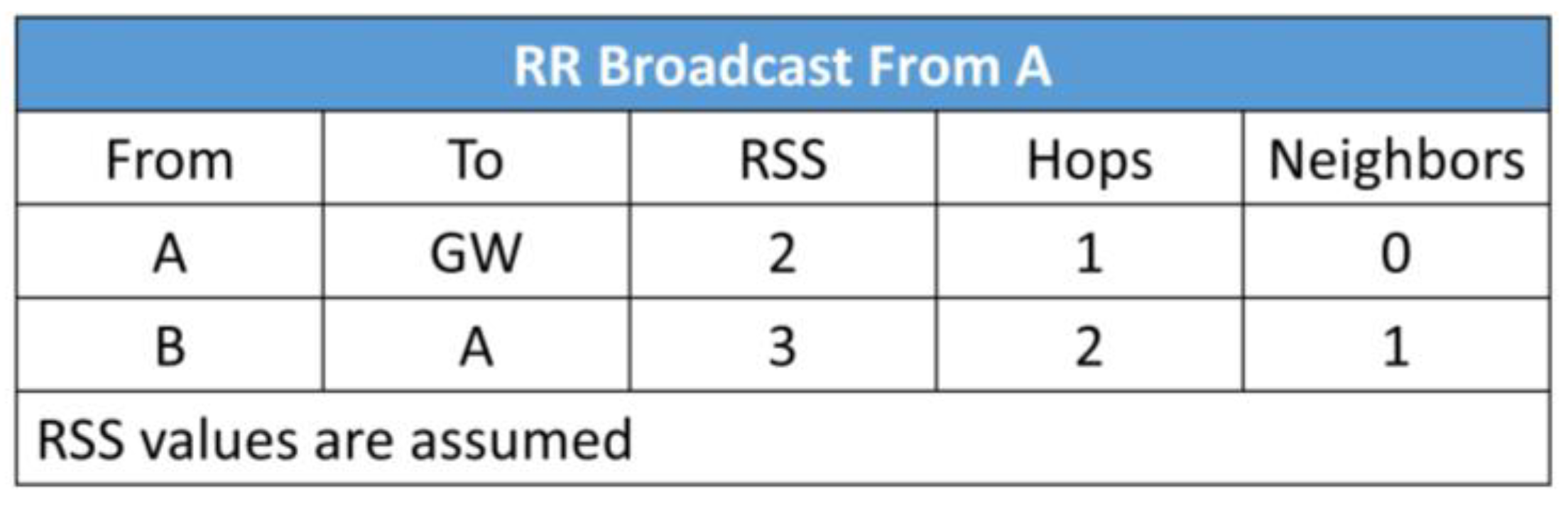
The process of route formation is initiated by the gateway node. The gateway broadcasts a route request (RR) packet, which will traverse throughout the network. When a node receives the RR packet, it measures the strength of the received signal. Initially, all the nodes will transmit at the same power, which will be enough to cover the maximum distance between the nodes. With the help of RSS, the distance between the RR sending node and receiving node is estimated. The RSS indicates the relative proximity between the sending node the receiving node. This is explained in the following example. Assume that three nodes, B, C, and H, are placed as illustrated in
Figure 5.
Suppose that nodes B and C have received the RR packet from the gateway. Nodes B and C will broadcast the RR packet at randomly selected time slots. Since H is the neighbor of both nodes, it will receive the RR packets from nodes B and C. When H receives the RR packet from B, it measures the RSS value and records it in a table. Similarly, H records the RSS value when it receives the RR packet from C. After that, it will compare the RSS value of both B and C, and will choose the node which has the stronger RSS. In this case, H will choose C as the next hop to forward the packet towards the gateway, because it has stronger RSS compare to B. The H node chooses the node having stronger RSS because it assumes that strong RSS is due to the shorter distance. However, before making the final decision, H will consider both RSS values, the number of hops between the candidate nodes and the gateway, and the number of neighbors of the candidate nodes.
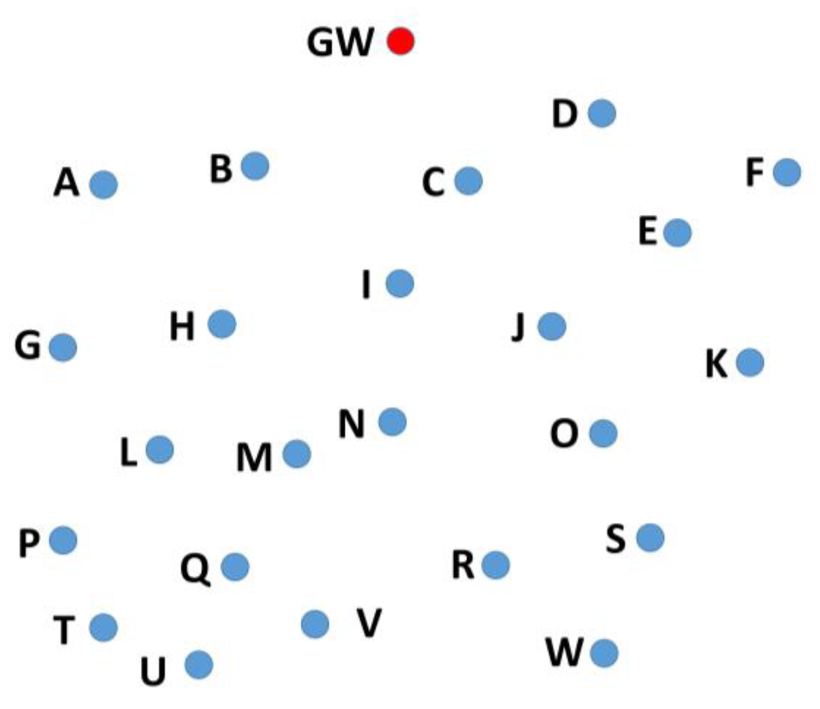
In the case of a short distance between the sender and the receiver, less transmission energy is required by the sender to transmit the packet. Therefore, when the weight of the RSS is set to maximum (i.e., 1), the closer candidate node is selected. This saves energy at the sender node. However, this approach may decrease the throughput if too many hops are added in the path between the original packet sender and the gateway. Therefore, two more metrics are considered at the time of selection of the forwarding node: number of hops and number of neighbors. The first one is because the number of hops affects the energy consumption and throughput. The second one is because a high number of neighbors means a better chance to be selected as the forward node, so it is a good metric to be considered. To better understand the idea, a scenario is considered. Suppose that a node, V, has two candidate nodes, Q and M, as shown in
Figure 6. Node Q is 300 m away from node V, has five neighbors (U, T, P, L, M) and can reach the gateway in four hops (L–H–B–GW), whereas node M is 600 m away from node V, has four neighbors (Q, L, H, N) and can reach the gateway in three hops (H–B–GW). At the time of forwarding node selection, node V will select the node based on all three metrics. The weights given to each metric will influence the selection accordingly. The selection is based on these three metrics to achieve a good balance between the throughput and the energy consumption. Suppose the shortest distance is given the highest weight, then node Q will be selected. If number of neighbors is given the highest weight, then node M will be selected, and if number of hops is given the highest weight then again M will be preferred over Q.
The values of the metrics will be normalized and multiplied by their weights (from 0 to 1). Prior to the deployment of the nodes, the weights will be assigned for each metric of selection.
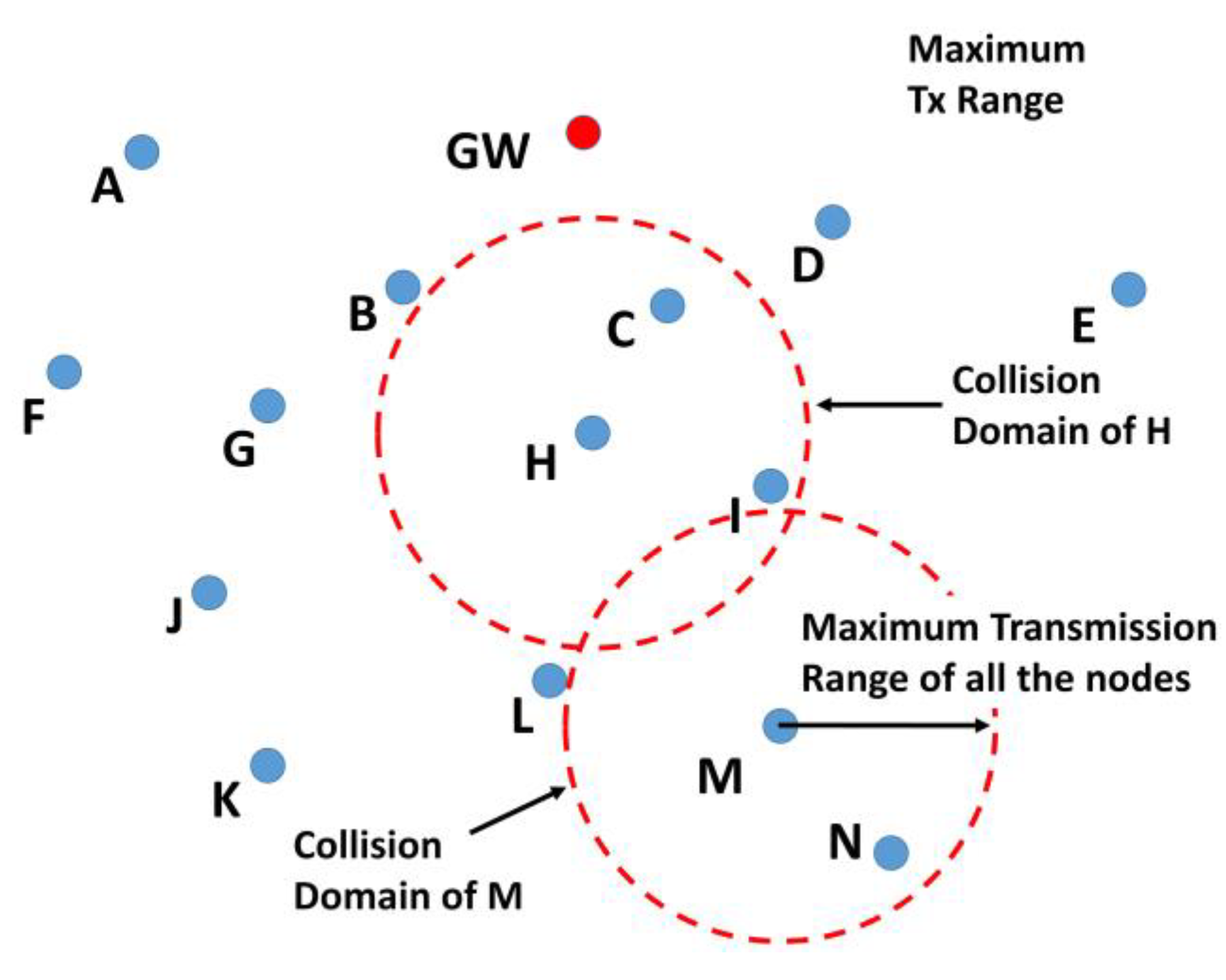
Packet collision at the receiver causes packet loss. The collision occurs when two or more nodes send packets to a node such that the packets arrive at the receiving node overlapped in time. All the nodes which can cause a collision in their transmission range form a collision domain, as shown in
Figure 7. A network may have multiple collision domains. The number of nodes in a collision domain depends on the node’s density and their transmission range. In order to avoid a collision, the nodes will send the RR packet at a randomly selected time slot from a set of possible time slots. Twenty time slots in the set are assumed to be sufficient for a moderately dense network. However, the number of slots may be increased in a densely populated network. The interval between two consecutive time slots will comprise packet delay, propagation delay, and guard time. For the latter, we assume that 5% of the total of packet delay and propagation delay will be enough to adjust the variance of the end to end packet transmission delay due to variations in the acoustic propagation velocity. When a node sends the RR packet, it will wait for the Route Request Acknowledgement (RR_ACK) packet from at least one node.
Once the RR packet has gone through all the nodes in the network, the nodes at end of the network send a Route Request Response RR_RSP packet back to the gateway. Nodes assume they are end nodes when they do not receive any response packet after sending the RR packet. When the gateway receives the RR_RSP packet from all the first hop nodes it assumes that all the nodes have successfully formed the path to the gateway. The nodes keep measuring the RSS of the received packets during the data packet transmission to optimize the path. If a node finds a closer neighbor compared to the existing forwarding node, then the former selects the latter as the next hop to forward the packets.
5. Mathematical Analysis
The criteria for path selection are quite straightforward. A node will prefer to form the routing path with the node that has the minimum distance, least number of hops, and least number of neighbors.
The combined values of these parameters are calculated based on the weight given to each parameter. If transmitting power is to be conserved, then signal strength will be given the maximum weight, whereas if the higher throughput is the objective then the least number of hops will be given the maximum weight. Hence, when a node receives the RR packet from multiple nodes
, it stores the signal strength of the received signal (
), the number of hops between the gateway and the node which sent the RR packet (
), and the number of neighbors (
). We propose to use a new score function
evaluated for every node
to make the forwarding node selection. The expression of
is given as follows:
where
,
, and
are the weights for RSS, hops, and neighbors, respectively. The sets of normalized values of RSS, number of hops, and number of neighbors are given by the following expressions, respectively:
A node
with a score
will be selected as the forwarding node when it fulfills the next rule:
Received signal strength (
) is calculated by:
where
is the transmitted signal power in logarithmic units, and
is the transmission losses, also in dB. The
parameter is calculated by:
where
is the distance between the nodes. The absorption coefficient α (in dB/km) is calculated by [
21]:
where
is the frequency (kHz).
7. Computer Simulation Results
Simulations were carried out using MATLAB® to estimate two efficiency parameters: the average delay from sending nodes to the gateway, and the average number of hops that each node employed to reach the gateway.
The simulation parameters are given in
Table 3.
The average number of hops and delays were simulated for different weight combinations of RSS, number of hops, and number of neighbors. The starting weight was 0.2 and increased to 1 with steps of 0.2. The weight combinations used in the simulation are given in
Table 4.
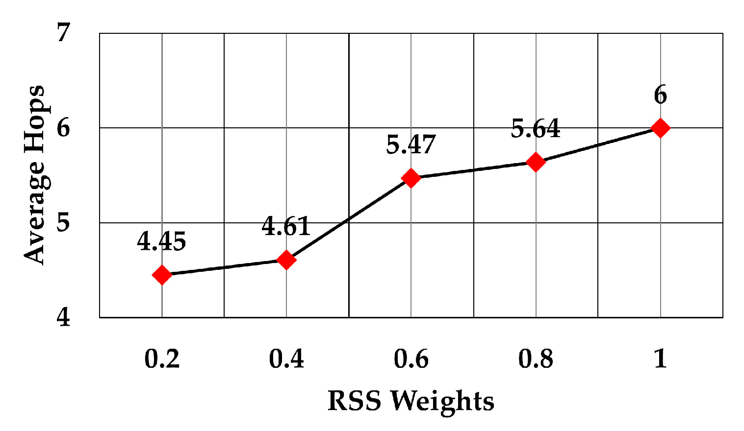
The average number of hops for RSS weights 0.2 to 1 is shown in
Figure 12. The graph shows that the average number of hops increased as RSS weight increased. This means that a node selects the forwarding node which closer to it, although it may have more nodes in the routing path to the gateway. The increase in the number of hops was approximately 34.83% as the RSS weight increased from 0.2 to 1 (6 versus 4.45 average hops).
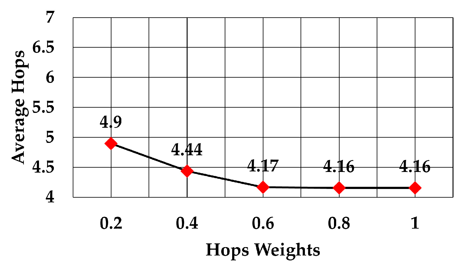
The average number of hops using weights between 0.2 to 1 is shown in
Figure 13. The graph shows how that figure decreased as the weight increased. This means that a node prefers to select the forwarding node which needs a smaller number of hops to reach the gateway. In this case, the throughput increased due to the smaller number of hops to reach the gateway, although this may increase the average energy consumption per node. Also, the average number of hops became almost constant after 60% weight of hops. Comparison of the average number of hops to reach the gateway when the RSS weight was the maximum (the other two weights were zero) and when the number of hops weight was the maximum (the other two weights were zero) shows that the average number of hops decreased by more than 30% (6 versus 4.16 average hops).
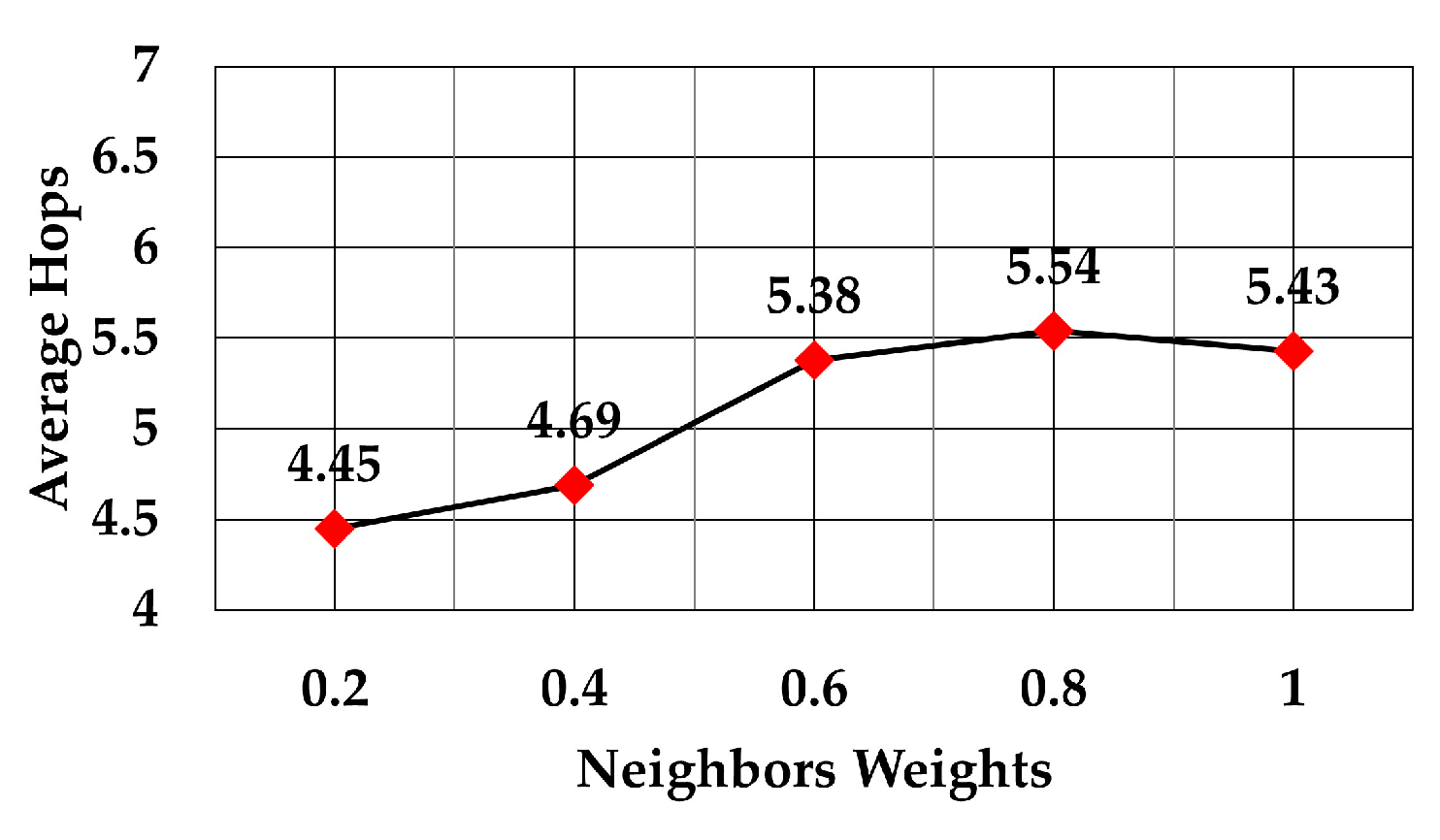
When the weight for least number of neighbors went from 0.2 to 1, the graph shown in
Figure 14 was obtained. Like in case of RSS, the average number of hops increased as the weight for least number of neighbors increased.
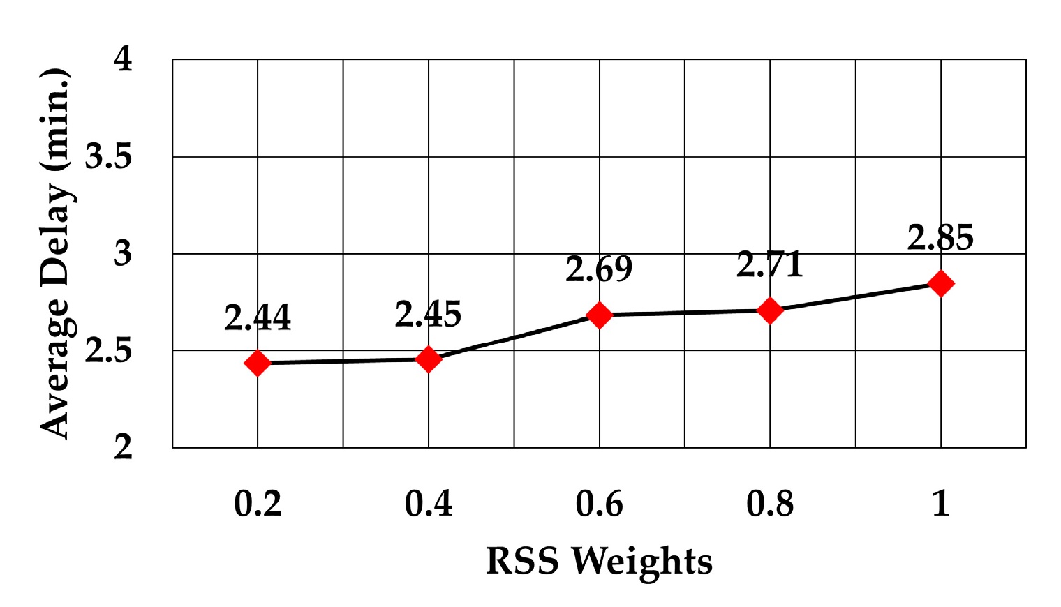
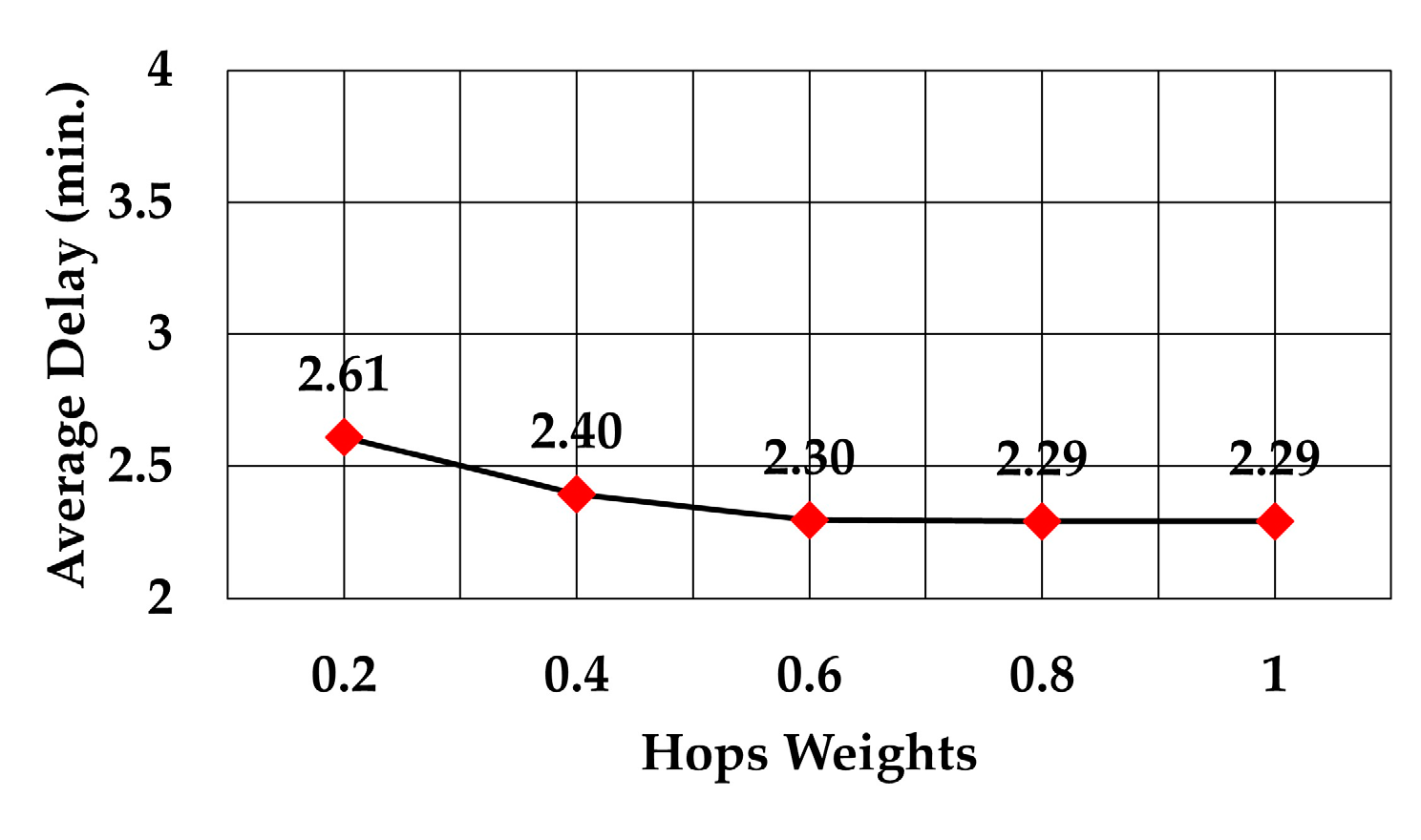
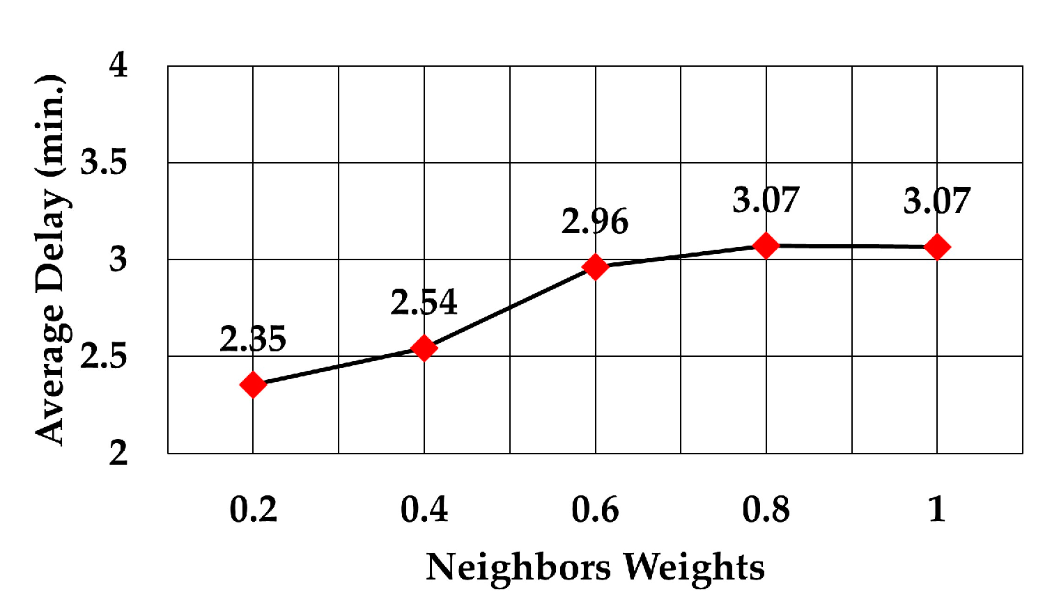
The analysis of packet delay from the node sending data to the gateway showed that it followed the same trend as the average number of hops, as can be observed in
Figure 15,
Figure 16 and
Figure 17. In the case of the least number of hops, the maximum weight decreased the delay by 12.2% compared to delay at weight = 0.2 (2.29 versus 2.61 min), 19.6% compared to delay at the maximum weight of RSS (2.29 versus 2.85 min), and 25.4% compared to delay at the maximum weight of least number of neighbors (2.29 versus 3.07 min).
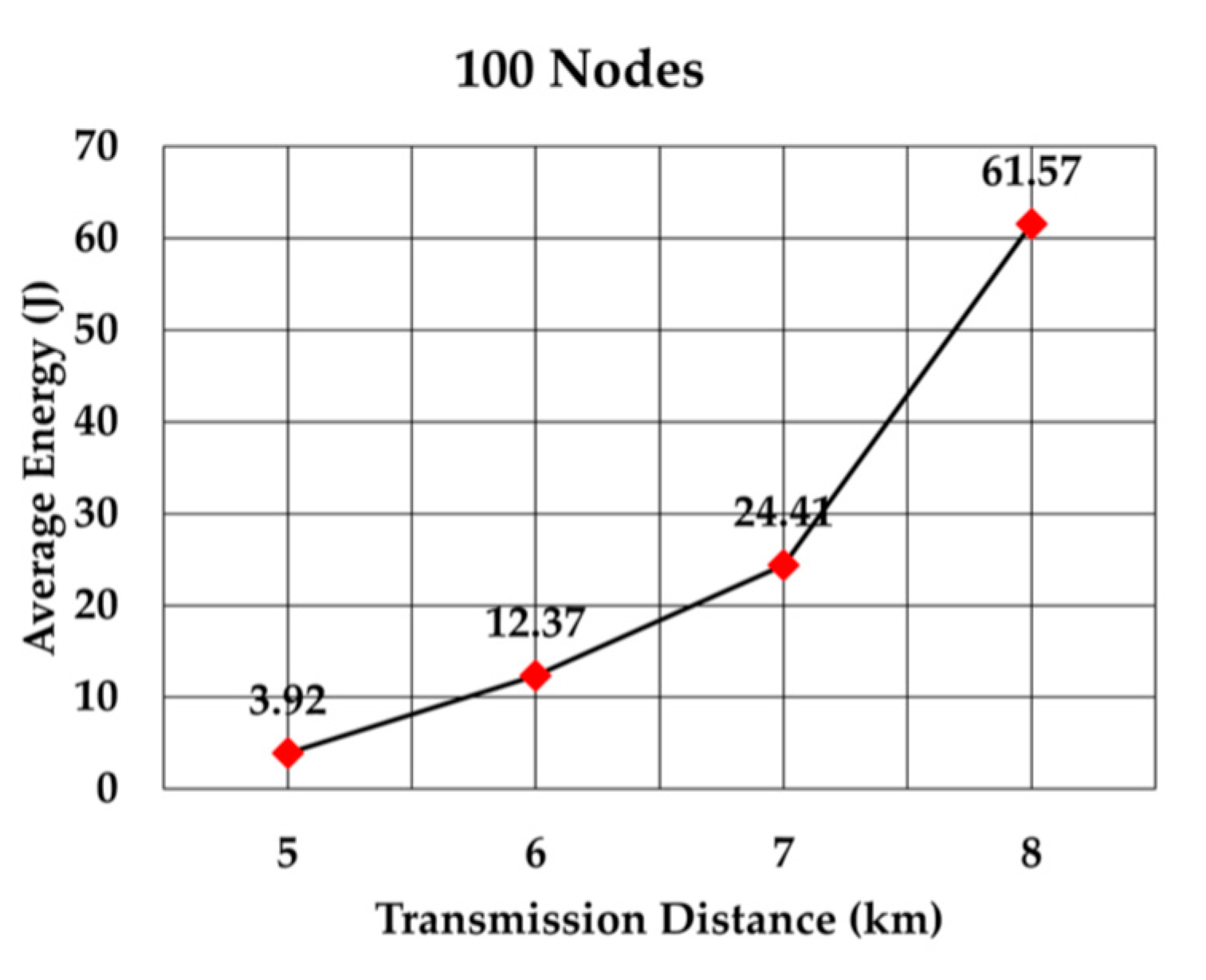
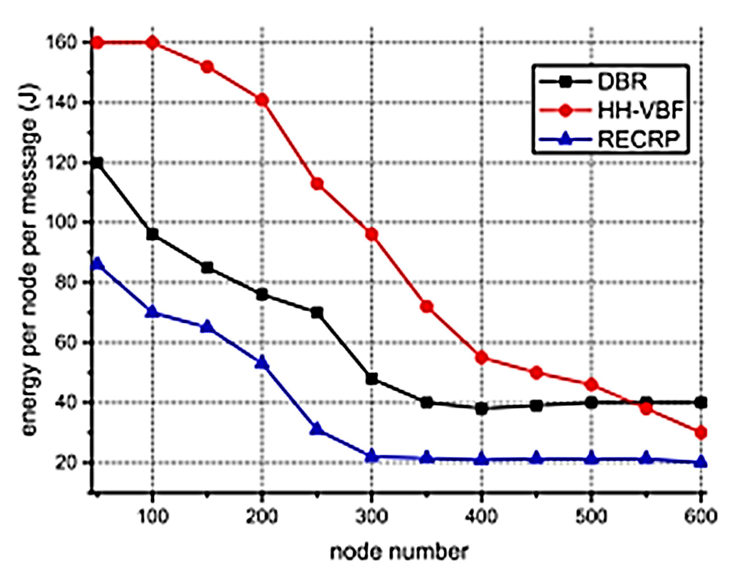
The average energy consumption of a node to send a data packet was analyzed for multiple densities of the nodes. To compare with values given in RECRP [
7] we assumed the same simulation parameters. The network area was 10 km × 10 km × 10 km and the number of nodes was 100, 200, 300, 400, 500, and 600. The data packet size was 256 bits and the transmission range was adjusted according to the node’s density. The average energy consumption for multiple transmission range for each number of nodes was simulated as shown in
Table 5. The simulation was run 10 times for each transmission range.
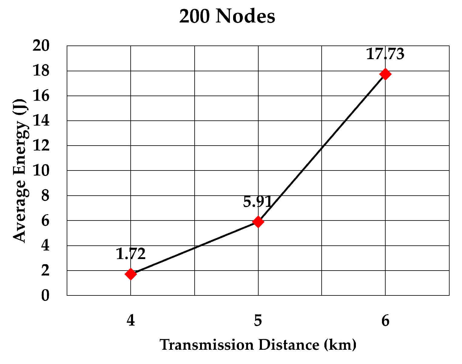
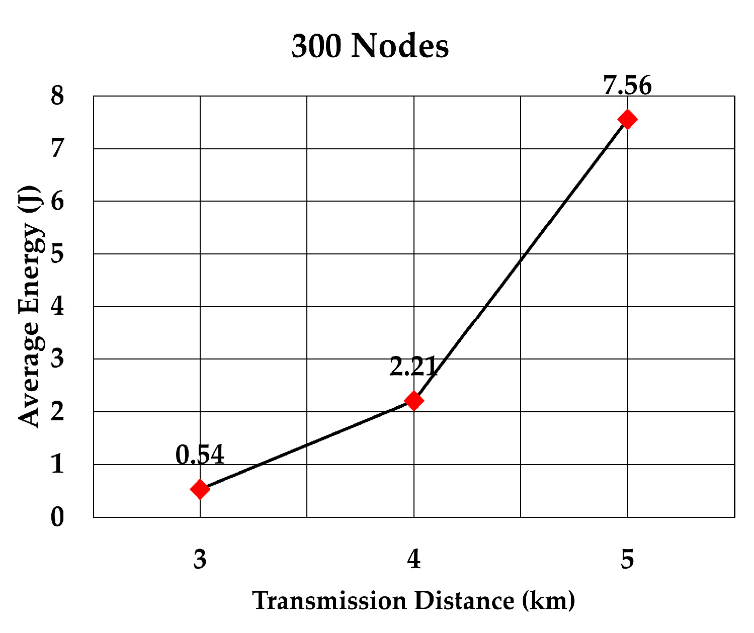
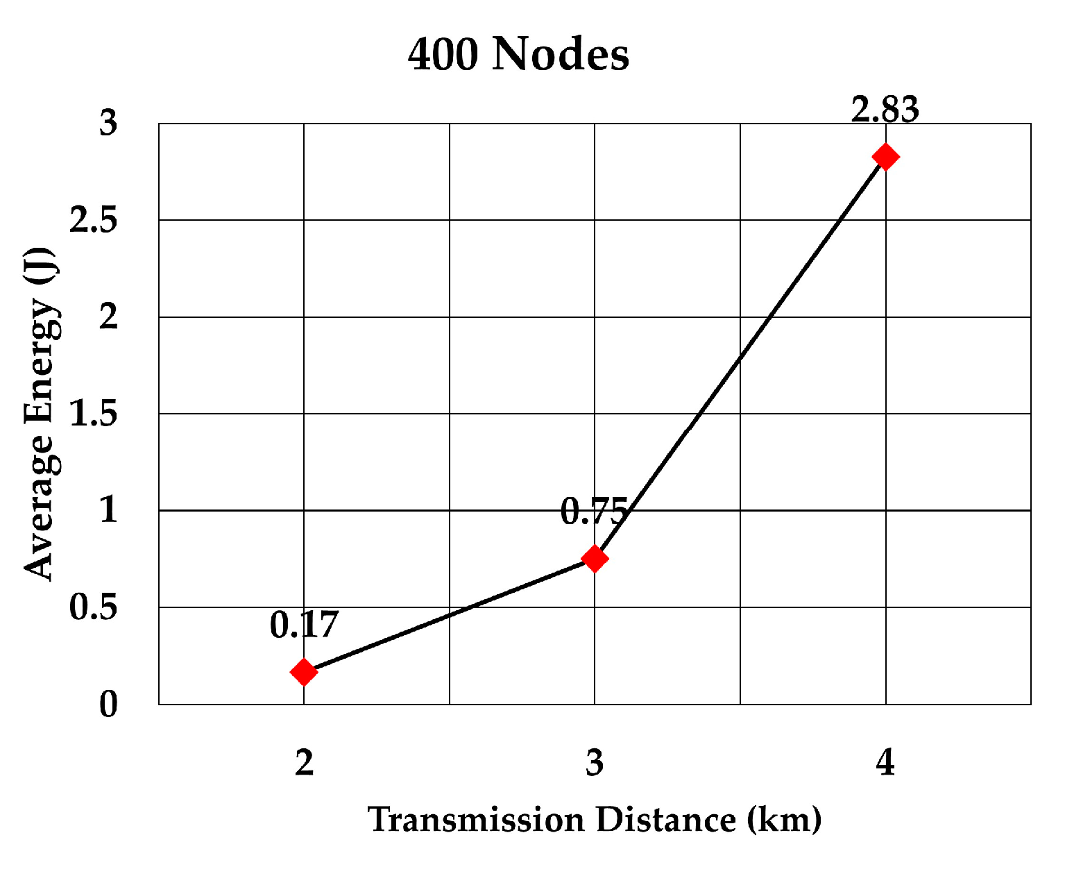
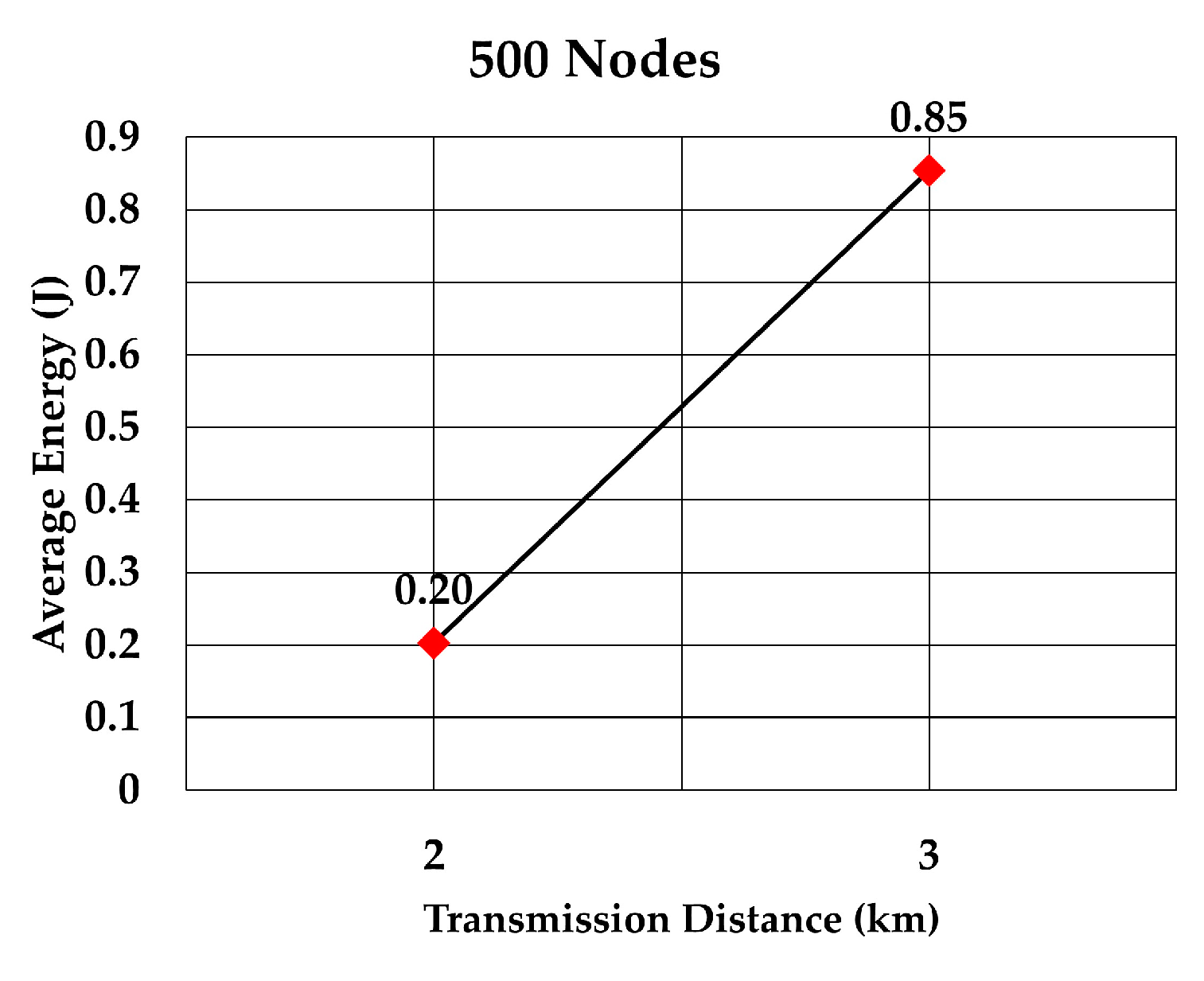
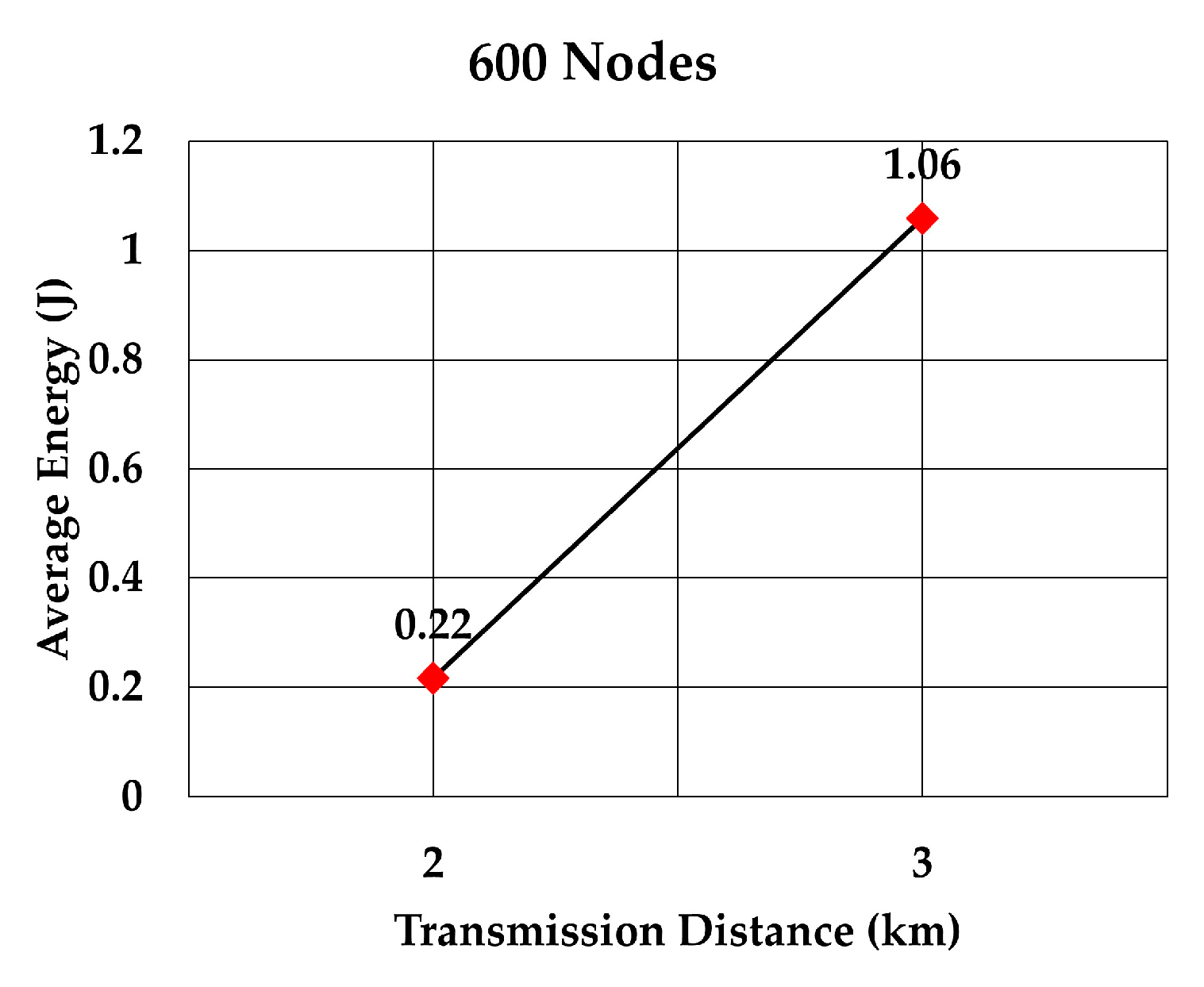
The average energy consumption per node per packet for 100, 200, 300, 400, 500, and 600 nodes is shown in
Figure 18,
Figure 19,
Figure 20,
Figure 21,
Figure 22 and
Figure 23, respectively. As we expected, the energy consumption increased as the transmission range increased.
Our proposed protocol is very close to RECRP but there are subtle differences. RECRP is a reactive protocol, whereas our proposed protocol is based on proactive approach. One of the RECRP forwarding nodes selection metrics is the residual energy of the candidate nodes. Instead of residual energy, we considered the number of data packets which a candidate node will have to forward. If a candidate node is already selected as a forwarding node by many neighbor nodes, then it will increase the energy consumption of the forwarding node and decrease the throughput. In order to keep the data traffic balanced among the nodes, the number of neighbors for each node is also a metric for node selection. Our proposed protocol can be maximized in terms of transmission energy by selecting the nodes with the shortest distance. The number of relay nodes between the data sending node and the sink node increases the delay and decreases the throughput. Therefore, our proposed protocol can be maximized to increase the throughput by minimizing the relay nodes. We can also optimize the protocol for energy efficiency by selecting the appropriate weights for distance and number of neighbors, and in the case of throughput, by selecting the appropriate weights for number of hops.
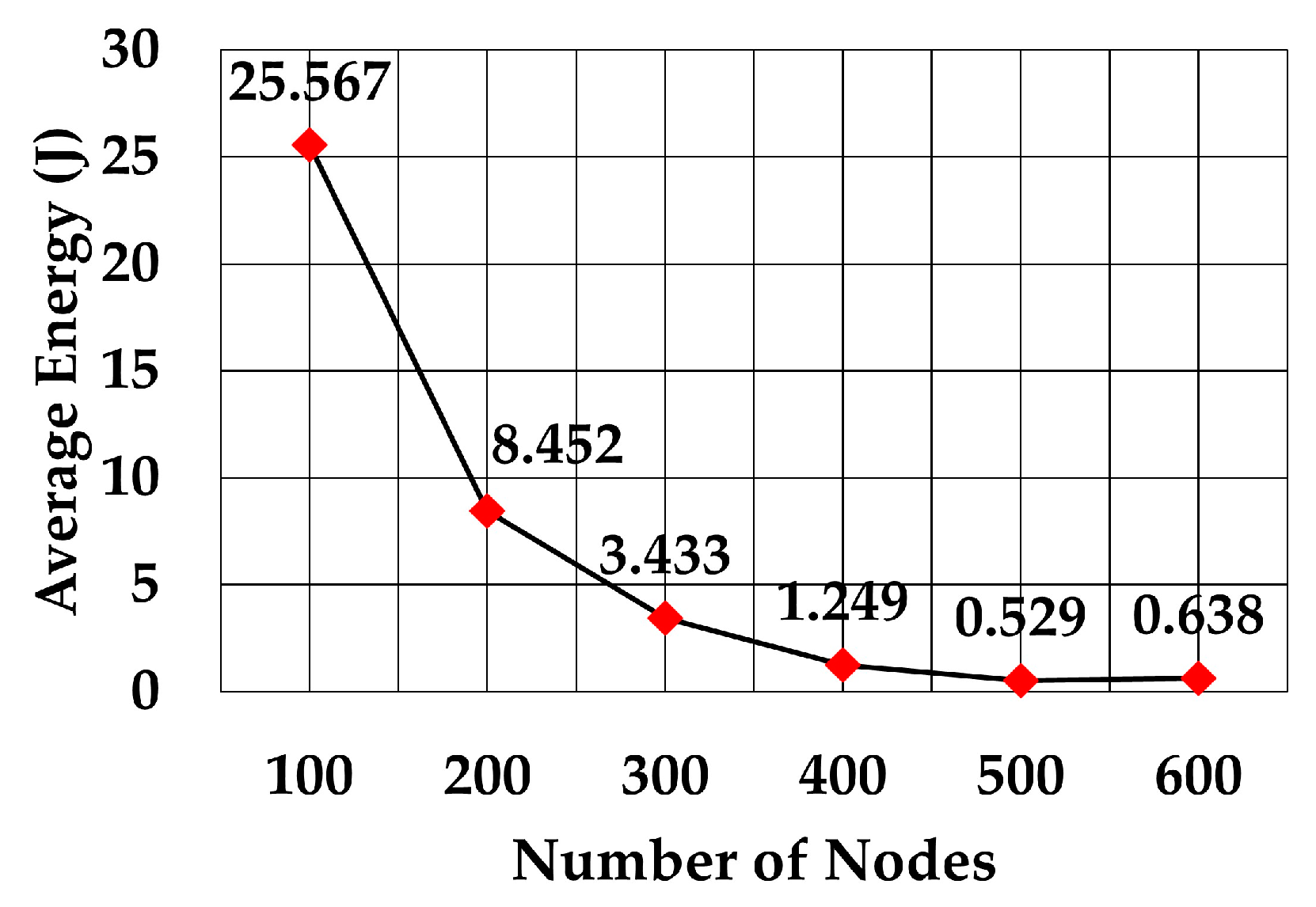
The energy consumption of SPRINT is shown in
Figure 24 and energy consumption by RECRP is shown in
Figure 25 (taken from [
6]). From the comparison of the two graphs, it is obvious that the energy consumption of SPRINT is much lower than RECRP under the same simulation conditions.
The values for RECRP have been tabulated from
Figure 23 (approximately) and compared to SPRINT simulations in
Table 6.
8. Conclusions
In this paper, we presented a routing protocol for randomly deployed underwater network. The sensor nodes are deployed randomly to monitor the environment or to warn of natural disasters, like tsunamis. The protocol is designed to optimize the data throughput and energy consumption of the sensor nodes. This protocol does not require additional sensing devices to ascertain the location. Hence, the proposed routing protocol is based neither on the location of the nodes nor on the topology of the network.
SPRINT is a proactive protocol to minimize the routing delay. Each node that wants to send a packet knows the forwarding node in advance. At regular intervals, when a node receives the data packet, it computes RSS, hops, and neighbors to optimize the routing path and overcome the issue of a dead node. This regular update of the routing path makes the protocol resilient and more efficient. However, computing routing path parameters upon receiving each data packet will increase the energy consumption significantly, therefore the routing path update will be carried out after certain number of data packets, depending on the arrival rate.
Energy consumption is low due to the adaptive transmission power, which is adjusted with the help of RSS estimation. Throughput can also be increased by reducing the relay nodes between the data source node and the gateway. Data traffic among the relay nodes is distributed evenly by considering the number of neighbors at the time of forwarding node selection.


