1. Introduction
Nowadays, with the popularity of unmanned vehicles, the navigation problems inherent in mobile robots are garnering even greater attention, among which the localization or calibration between different sensors is one of the basic problems. To fully utilize the information from sensors and make them complementary, the combination of 3D and 2D sensors is a good choice. Thus, the hardware devices of those systems are usually based on cameras and Light Detection and Ranging (LiDAR) devices. Comparing the two sensors, a camera is cheap and portable, and it can obtain color information about the scene, but it needs to correspond to feature points during calculation, which will be time consuming and sensitive to light. LiDAR can get 3D points directly and has an effective distance of up to 200 m. In addition, LiDAR is suitable for low-textured scenes and some scenes under varying light conditions. However, the data are sparse and lack texture information. When using a combination of cameras and LiDAR, it is necessary to obtain transformation parameters between coordinate systems of the two kinds of sensors. Once the transformation parameters, i.e., the rotation matrix and translation vector are obtained, the two coordinate systems are aligned, and the correspondence between 3D points and the 2D image is established. The 3D point cloud obtained by the LiDAR can be fused with the 2D image obtained by the camera.
The existing target-based methods require users to prepare specially designed calibration targets such as chessboard [
1], circular pattern [
2], orthogonal trihedron [
3], etc., which limits the practicality of these methods. Target-less methods break through this limitation. These kinds of methods can be roughly divided into several categories according to work principles: odometry-based, neural network-based, and feature-based. The odometry-based methods [
4,
5] require many continuously inputted data, and the neural network-based methods [
6,
7] need even more data to train networks, and may lack clear geometric constraints. The feature-based methods usually use point or line features from scenes. Point feature is sensitive to noise, sometimes requiring user intervention to establish 3D–2D point constraints [
8]. Line feature is more stable, and 3D–2D line correspondence is usually required (known as the Perspective-n-Line problem) [
9,
10,
11]. However, in an outdoor environment, this correspondence is usually hard to be established. Because LiDARs are generally placed horizontally, many detected 2D lines on the image cannot find their paired 3D counterparts due to the poor vertical resolution.
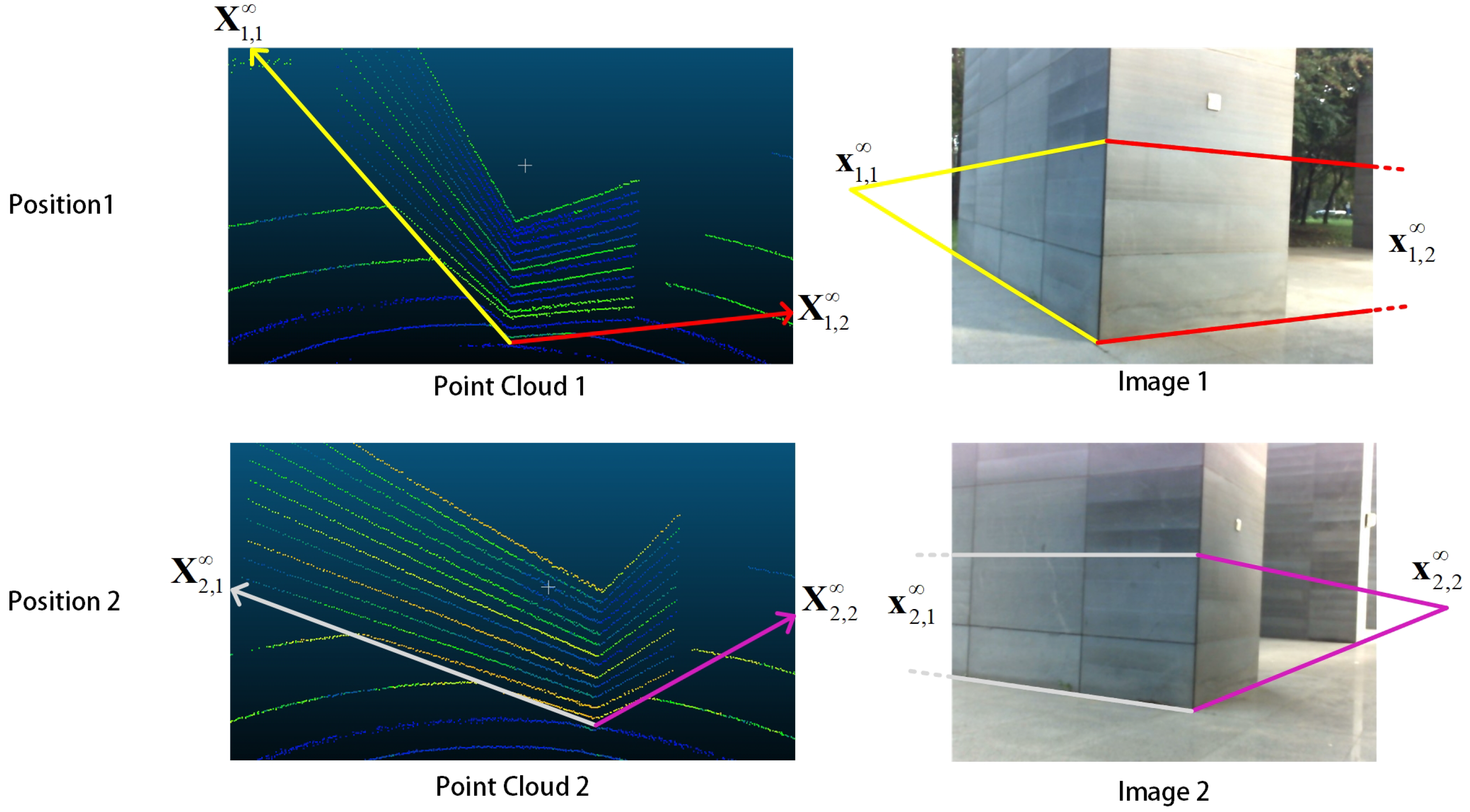
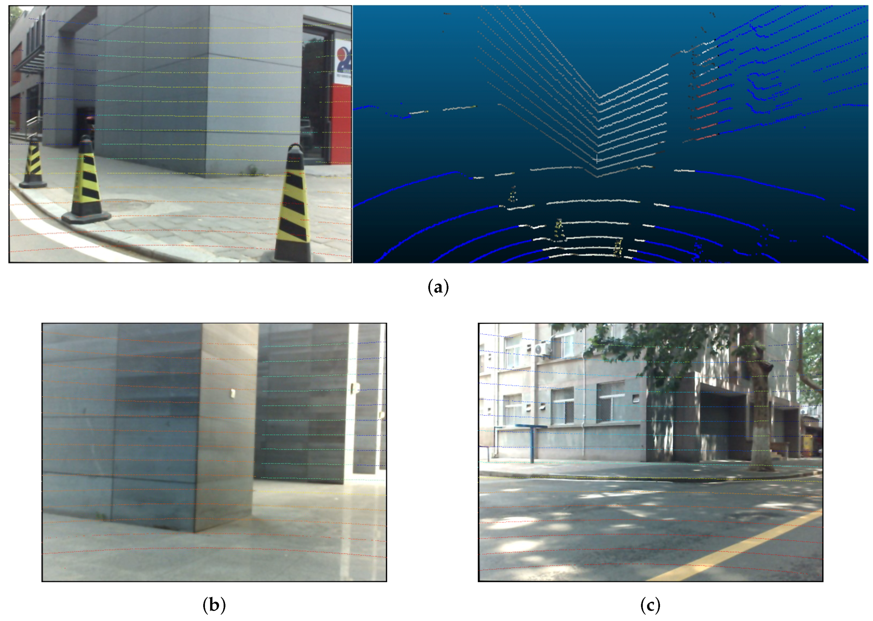
The main contribution of this paper is that we provide a novel line-based method to solve the extrinsic parameters between a LIDAR and a camera. Different from existing line-based methods, we take infinity points into consideration to utilize 2D lines, so that the proposed method can work in outdoor environments with artificial buildings, as shown in
Figure 1. As long as there are enough parallel line features in a scene, it can be chosen as calibration environment. In addition, our method only requires a small number of data to achieve sufficient results. We transform the correspondence of parallel lines into the correspondence between 3D and 2D infinity points. By getting and aligning the direction vectors from the infinity points, the rotation matrix can be solved independently in the case that the camera intrinsic matrix is known. Then, we use a linear method based on point-on-line constraint to solve the translation vector.
2. Related Work
The external calibration between two sensors is always discussed. According to the different forms of data collected by these two devices, researchers have been looking for appropriate methods to obtain conversion parameters between the two coordinate systems. In some methods, the target is a chessboard, which is a plane object. Zhang et al. [
1] proposed a method based on observing a moving chessboard. After getting points-on-plane constraints from images and 2D laser data, a direct solution was established to minimize the algebraic error, while they still needed several poses of planar pattern. Huang and Barth [
12] first used chessboard to calibrate a multi-layer LiDAR and vision system. Vasconcelos et al. [
13] formulated the problem as a standard P3P problem between the LiDAR and plane points by scanning the chessboard lines. Their method is more accurate than Zhang’s. Geiger et al. [
14] arranged multiple chessboards in space to obtain enough constraint equations from a single shot. Zhou et al. [
15] employed three line-to-plane correspondences, and then solved this problem with the algebraic structure of the polynomial system. Afterwards, they put forward their method based on the 3D line and plane correspondences and reduced the minimal number of chessboard poses [
16]. However, the boundaries of the chessboard should be determined. Chai et al. [
17] used ArUco marker, which is similar to the chessboard pattern, combined with a cube to solve the problem as a PnP problem. Surabhi Verma et al. [
18] used 3D point and plane correspondences and genetic algorithm to solve the extrinsic parameters. An et al. [
19] combined chessboard pattern with calibration objects to provide more point correspondences. However, those methods require the checkerboard pattern.
When spatial information is taken into account, some methods based on special calibration objects are proposed. Li et al. [
20] provided a right-angled triangular checkerboard as calibration object. By using the line features on the object, the parameters can be solved. Willis et al. [
21] used a sequence of rectangular boxes to calibrate a 2D LiDAR and a camera. However, the settings for the devices are demanding. Kwak et al. [
22] extracted line and point features which are located on the boundaries and centerline of a v-shaped target. Then, they obtained the extrinsic parameters by minimizing reprojection error. Naroditsky et al. [
23] used line features of a black line on a white sheet of paper. Fremont et al. [
2] designed a circular target. In the LiDAR coordinate system, they used 1D edge detection to determine the border of the target and fitted the circle center and plane normal, but the size of the target needs to be known. Gomez-Ojeda et al. [
3] presented a method that relies on an orthogonal trihedron, which is based on the line-to-plane and point-to-plane constraints. Pusztai et al. [
24] used boxes with known sizes to calibrate the extrinsic parameters between a LiDAR and camera. Dong et al. [
25] presented a method based on plane-line constraints of a v-shaped target composed of two noncoplanar triangles with checkerboard inside. The extrinsic parameters can be determined from single observation. These methods have high requirements for customized artificial calibration objects, and this may make them hard to be popularly adopted.
Some methods explored calibration methods without using artificial targets. These methods usually start with basic geometric information in a natural scene. Forkuo and King provided a point-based method [
26] and further improved it [
27], but the feature points are obtained by corner detector, which is not suitable for depth sensors with low resolution. Scaramuzza et al. [
8] provided a calibration method based on manually selecting corresponding points. However, too many manual inputs will cause the results to become unstable. Mirzaei et al. [
28] presented a line to line method by extracting the straight line structure. This algorithm is used for calibrating the extrinsic parameters of a single camera with known 3D lines, but it gives inspiration to the follow-up methods. Moghadam et al. [
9] used 3D–2D line segment correspondences and nonlinear least square optimization to establish the method. This method performs well in indoor scenes, but, in outdoor scenes, the number of reliable 3D lines may not be adequate because of the viewing angle, low resolution of depth sensors, etc. This may lead to situations where many detected 2D lines cannot find their corresponding 3D counterparts. Levinson et al. [
29] presented a method based on analyzing the edges on images and 3D points. This method only considers boundaries without extracting other available geometric information, and 3D point features may not be stable. Tamas and Kato [
30] designed a method based on aligning 3D and 2D regions. The regions in 2D and 3D are separated by different segmentation algorithms, which may lead to inaccurate alignments of segmented regions and affect result accuracy. Pandey et al. [
31] used reflectivity of LiDAR points and gray-scale intensity value of image pixels to establish constraints. By maximizing Mutual Information (MI), the extrinsic parameters can be estimated. Xiao et al. [
32] solved the calibration problem by analyzing the SURF descriptor error of the projection of laser points among different frames. This method needs to input the transformation relationship among a large amount of images in advance. Jiang et al. [
33] provided an online calibration method using road lines. They assumed that there are three lines which can be detected by both the camera and LiDAR on the road. This method is more similar to the following odometry-based methods and is suitable for automatic driving platform.
There are also some works based on other aspects (e.g., odometry and network). Bileschi [
34] designed an automatic method to associate video and LiDAR data on a moving vehicle, but the initial relative pose between the sensors is provided by an inertial measurement unit (IMU). Schneider et al. [
35] presented a target-less method based on sensor odometry for calibration. After this, they further gave an end-to-end deep neural method to calculate the extrinsic parameters [
6]. Taylor and Nieto [
4] presented an approach for calibrating the extrinsic parameters among cameras, LiDARs, and inertial sensors based on motion. Gallego et al. [
36] provided a tracking method based on event camera in high speed application environments, but this method requires special devices and is used in special circumstances. Park et al. [
5] aligned the odometry of the LiDAR and camera to obtain a rough estimation of extrinsic parameters, and then refined the results jointly with time lag estimation. These odometry-based methods require continuous input to estimate sensor trajectory, which demands many data. Cumulative errors are still a problem for odometry-based methods. However, they can work in targetless environments and are able to calibrate the extrinsic parameters continuously. With the development of neural networks, several novel methods appear. Schneider et al. [
6] offered RegNet, which is the first convolutional neural network to estimate extrinsic parameters between sensors. Iyer et al. [
7] presented a self-supervised deep network named CalibNet. Considering the Riemannian geometry, Yuan et al. [
37] recently designed RGGNet to estimate the offsets from initial parameters. Neural network-based methods need more data to train the networks, and the performance is closely related to the training data.
3. Method
Throughout this paper the LiDAR coordinate system is regarded as the world coordinate system. The translation relationship of one point
in the world coordinate system to the image point
is
where
is the intrinsic matrix of the camera. It can be easily calibrated by traditional methods, e.g., Zhang’s method [
38]. We aim to estimate the extrinsic parameters, i.e., rotation matrix
and translation vector
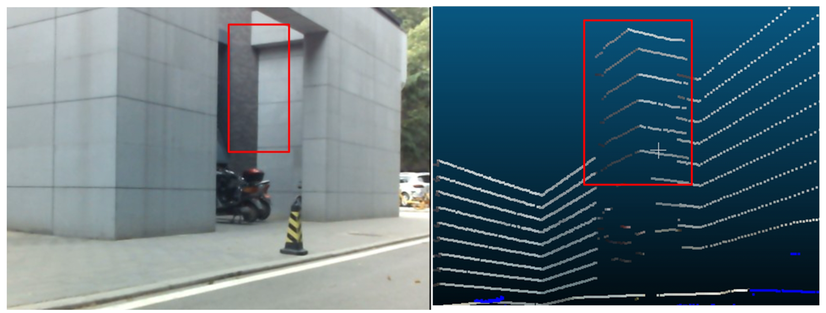
. To solve this problem, it is obvious that we need to find some features which can be detected in both the LiDAR point clouds and images. Considering robustness and commonality, line feature is an appropriate choice. In this paper, we choose the corners of common buildings to illustrate our method because they usually have sharp edges and available line textures, but this method can also be applied to any object with similar features. Some appropriate building corners are shown in
Figure 2. We define each spin of LiDAR as a frame. We also define a frame and its corresponding image as one dataset. It is recommended to keep the devices fixed while collecting a dataset to avoid the distortion brought by movement.
3.1. Solve Rotation Matrix with Infinity Point Pairs
To solve rotation matrices, direction vector pairs are usually required. Many target-based methods use chessboards as the calibration object because it is convenient to get normal vectors of board planes in both the camera and the LiDAR coordinate systems. However, the board plane is small, and the LiDAR points on it are noisy, which makes it difficult to get sufficient results from a small number of data. Considering there are enough parallel lines in common scenes, we can obtain the vector pairs through the 3D–2D infinity point pairs based on line feature.
One bunch of 3D parallel lines intersect at the same infinity point
, which lies on the infinite plane
in the space. Since 3D parallel lines are no longer parallel after perspective transformation, the intersection point of their projection lines is written as
, which is not at infinity [
39].
and
make up a 3D–2D infinity point pair. Here, we use L-CNN [
40] to detect the edges on an image. A RANSAC procedure is used to detect the infinity points of artificial buildings from images as in [
41,
42,
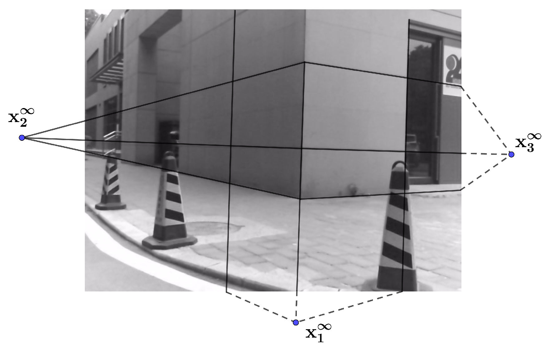
43]. Then, three bunches of lines and their intersection points
on an image plane as shown in
Figure 3 can be obtained. From Equation (
2), we can get three 3D unit vectors
,
and
.
When setting up the devices, an initial guess of the camera optical axis and LiDAR orientation can be obtained, i.e., a coarse relative pose of the LiDAR and camera is known. In the LiDAR point cloud, the planes of a building corner can be separated by existing point cloud segmentation methods [
44,
45,
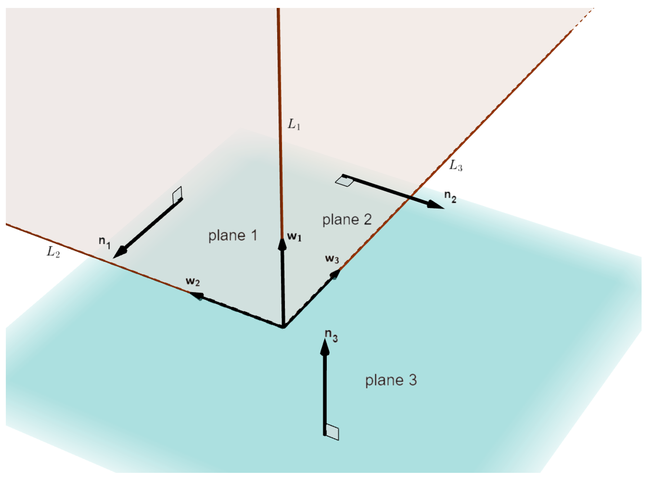
46]. The three planes shown in
Figure 4 can be extracted according to the known orientation. The RANSAC algorithm [
47] is used to fit the extracted planes. Then, we can get their normal vectors
,
and
:
, and
are the normalized cross products of the plane normal vectors. They are the direction vectors of the 3D lines
,
, and
, as shown in
Figure 4.
Equation (
5) shows the homogeneous form of the 3D infinity points in the LiDAR coordinate system. Notice that the direction (i.e., sign) of
is still ambiguous, as shown in Equation (
4). If
is determined from an image, the direction it represents in the environment is roughly obtained. Then, its paired
can be chosen by this condition, and the sign of
can also be determined (consistent with the direction of
).
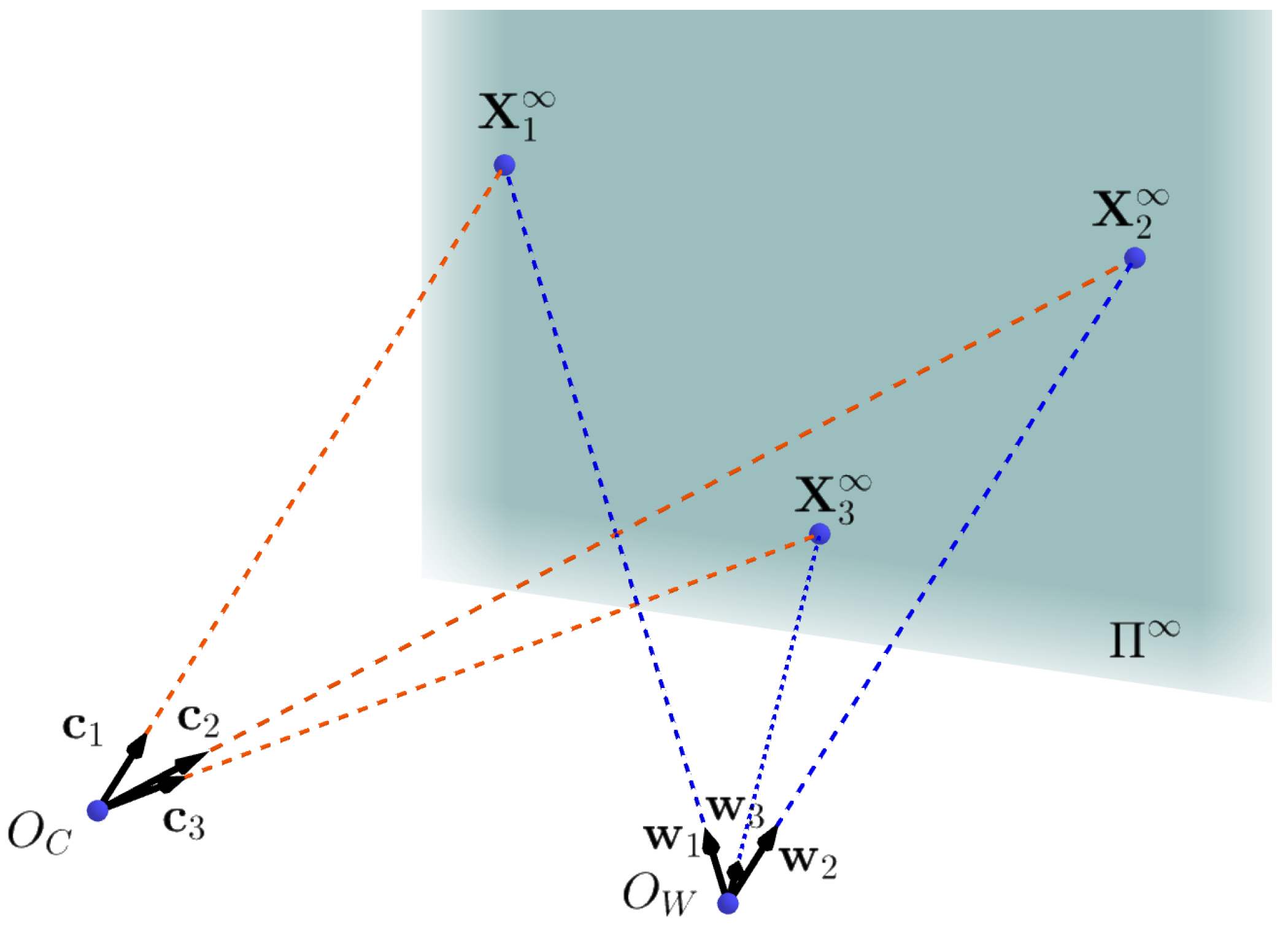
Figure 5 shows the relationship between the two coordinate systems.
Then, the direction vector pairs made up of
and
are obtained. The rotation matrix can be solved in close form with at least two pairs of direction vectors [
48,
49]. Assume there is a unit direction vector
in the world coordinate system. The relationship between
and its paired vector
is
. For the
i th pair, we have
. Let
Applying singular value decomposition to , we have and . The minimum number of n to determine is 2.
Furthermore, if we have three or more vector pairs,
can also be solved in a simpler way:
where
,
. The rank of matrix
must be greater or equal to 3 in this equation. Before computing
, the 3D infinity points should be checked to ensure that at least three directions in the space are selected. The solved
may not be orthogonal due to noise. To keep
as an orthogonal matrix, let
be
3.2. Solve Translation Vector
The method presented above allows us to estimate rotation matrix without considering translation vector . Taking as a known factor, here we use a linear method to get .
Assume that there is a 3D point
located on the line
L in the LiDAR coordinate system as shown in
Figure 6.
and
are the projections of
L on the normalized image plane
and image plane
, respectively.
is the normal vector of the interpretation plane
. We can obtain
easily from
through the known intrinsic matrix of the camera. For each pair of corresponding lines, we have one equation for
[
50]:
With the fitted planes in Equation (
3), the 3D wall intersection lines
,
, and
are easy to obtain, as is the 3D point
, which lies on the 3D line. We choose
in the LiDAR coordinate system and
on the image as corresponding line pairs. In general case, if three different sets of corresponding line pairs are known, the translation vector
can be solved. However, in our scene,
,
, and
intersect at the same point on the image plane. This leads to a case that the three equations based on line constraint are not independent [
51]. Thus, the equation factor matrix cannot be full rank, and this makes it difficult to solve
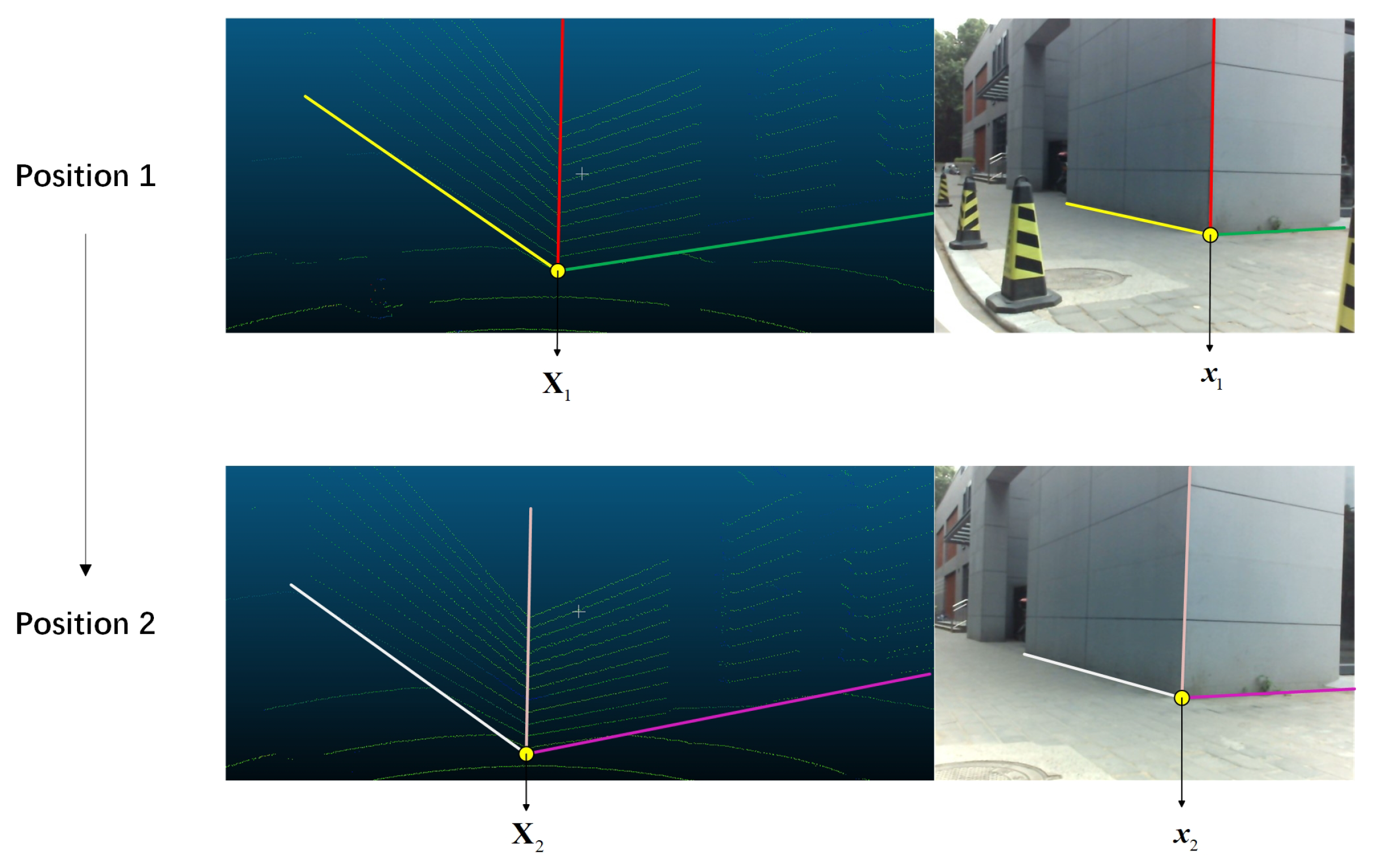
from a single dataset. To avoid this, we choose to move the LiDAR and camera and use at least two datasets to compute
. An example is shown in
Figure 7, and then we can choose any three disjoint lines from these data to solve the problem.
3.3. Optimization
To make the results more accurate, the minimum of
and
under some constraints needs to be found. In this part, we construct cost function and then minimize the reprojection error to optimize
and
. We use the intersection of lines to establish the constraint. Assume that we have collected
datasets. For each set, we can get the intersection points
and
of the 2D and 3D lines, as shown in
Figure 7. The cost function is:
We solve it by nonlinear optimization methods, such as the Levenberg–Marquard (LM) algorithm [
52]. For the initial solutions with very low accuracy, we regard them as outliers and reject them before optimizing. The filter procedure is based on the RANSAC algorithm; a distance threshold for the reprojection error is set to distinguish the initial solutions. In this way, we can solve
and
and remove the influence from noise as much as possible. The complete process for the algorithm is described in Algorithm 1.
| Algorithm 1: |
![Sensors 20 06319 i001]() |
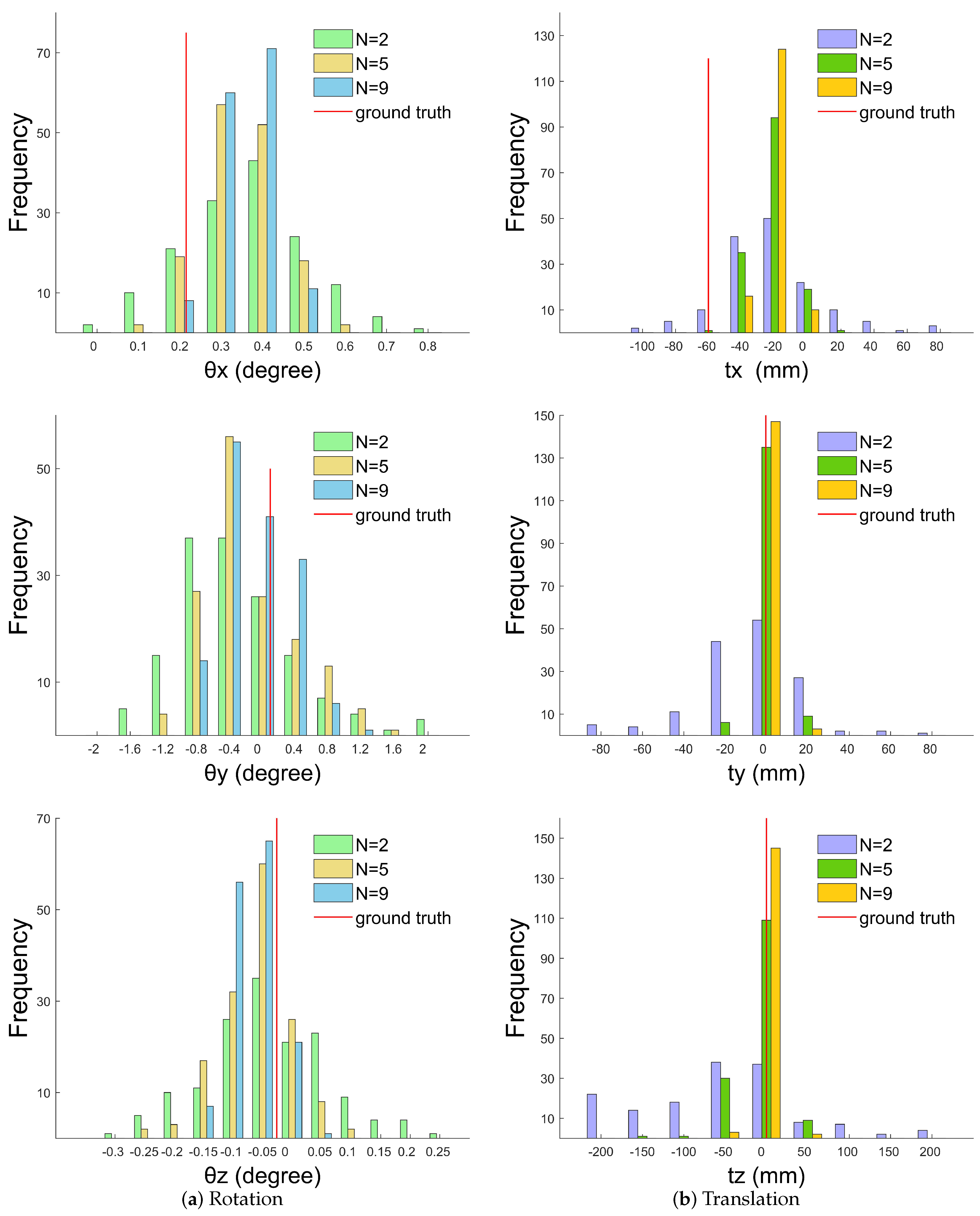
Similar to Fremont’s work [
2], we estimate the precision of the calibration solution by the Student’s
t-distribution. The covariance matrix
of the estimated parameters is defined as follows:
where
is an unbiased estimate of the variance and
is the Jacobian matrix of the last LM algorithm iteration. Then, the width of confidence interval is given by:
where
is the standard deviation of the
ith parameter.
is determined by the degrees of freedom of the Student’s
t-distribution and confidence (e.g.,
).


