1. Introduction
Pain phenomenon is a composition of perceptual and affective components reflected by individual experience [
1]. Questionnaire-based rating is a standard measurement to assess pain in clinical studies, but it is not only subjective but also impossible for people who cannot feel or express the pain. Moreover, it is difficult to measure the temporal change of pain perception. There have been several research efforts on objective evaluation of pain. Multiple vital signs and surrounding conditions have been integrated to estimate the perceived pain levels [
2]. However, the source signals are mostly the secondary or indirect effects of the pain itself. Thus, the effectiveness of the approach needs to be further confirmed.
Electroencephalography (EEG), which contains the information of most motor-sensory activities and cognitive processes, provides a signal source for an alternative approach. EEG recordings are particularly important in the diagnosis of epilepsy [
3] and in brain computer interface (BCI) [
4]. Several studies have shown that using EEG analysis can reveal pain responses from various stimulations such as heat or cold [
5,
6,
7], electrical ones [
8,
9] and laser [
10,
11]. Components of pain-event related potential (pain-ERP) were used as signals to estimate pain perception of healthy subjects [
7,
8]. Power spectrum density and power based on time-frequency representation have been used to estimate different pain levels and predict central neuropathic pain [
12,
13,
14]. Thus, EEG was subsequently applied as a valid modal for quantifying pain. Ozgul et al. [
15] and Gram et al. [
7] found that pain-ERP has a high test-retest-reliability for pain on healthy participants.
Table 1 shows a summary of the previous studies on the classification of high pain and low pain caused by different types of pain stimulations, from different EEG analysis. Based on the information in
Table 1, it is noticed that although some classification models have been developed, and high accuracy has been achieved using time-frequency representation of EEG signals for multiple classes of cold pain [
16,
17,
18], none of the studies so far have achieved high classification accuracy from feature vector of pain-ERP for multiple pain perception levels. The reason may lie in the lack of the investigation on the component of classification, feature extraction and selection. Especially, the feature or feature groups that could present the real nature of the pain-ERP, while keeping its robustness to the noise in the EEG signals, need to be explored. In clinical practice, different pain scales such as Visual Analog Scale (VAS), Verbal Rating Scale (VRS), Numerical Rating Scale (NRS) etc. [
19], have been used to evaluate the pain levels. Though relying on subjective feedback, they are either continuous or multiple-level (4–10 levels) evaluation. In the studies on mutual validation of different types of pain scales [
20], four levels (no pain, mild pain, moderate pain, severe pain) were investigated. Therefore, the multiple-level classification is important for realizing objective pain level assessment for clinical practice, which is our ultimate goal.
On the other hand, to deal with the nonlinear dynamical aspects of brain waves, nonlinear analysis of EEG has been used for determining disorder symptoms. In the work presented by Jelles et al. [
22], the correlation dimension underlying EEG signals was calculated and found pronouncedly decreased for Alzheimer patients. Additionally, Tzimourta et al. [
23] calculated linear and nonlinear features extracted from EEG for developing mini-mental state examination score for Alzheimer’s disease. Besides, EEG analysis based on nonlinear features (including Lyapunov exponent and Lempel-Ziv complexity) was useful for differentiating depression from normal mental states [
24,
25]. According to the fractal nature of EEG signals [
26], fractal dimension may be useful for estimating pain perception levels. Fractal dimension is an index used for measuring the complexity of the brain in different states [
27], which has many computational techniques such as Higuchi’s fractal dimension (HFD), Hausdorff dimension, Grassberger-Procaccia correlation dimension (GP), Entropy, etc. HFD and GP were selected to analyze EEG signals corresponding to different pain conditions in this study. Both of them examine the dimensional complexity of signals in time domain [
27]. HFD evaluates the complexity without reconstruction of a strange attractor, which can provide accurate estimation and does not rely on a binary sequence [
28]. GP is widely-used for dimension measurement in time series analysis, through phase space reconstruction to distinguish irregular time series generated by noise from nonlinear deterministic signal sources [
29,
30].
Furthermore, applying feature selection to choose the right set of features is important to improve the performance of supervised models like classification in this study. In the literature [
31], regarding feature selection for supervised models, features can be selected by wrapper methods and embedded methods, in which feature selection is tightly coupled with the model fitting process. The difference lies in that subsets of features are evaluated by total task performance in the former method, or by a certain feature-level regularization criterion (such sparsity) in the latter one. In this study, filtering method, in which feature selection is independent of the model fitting process, and subsets of features were evaluated by different types of criteria (such Relief, Akaike’s Information criterion, Chi-squared score, and Fisher score, etc.) reflecting their inherent characteristics, was employed, for avoiding the overfitting problem and computation cost that may be caused by the wrapper and embedded methods. Fisher score was used to choose the most discriminant features, while reducing the dimensionality of feature space [
32,
33].
In this study, our hypothesis is: features based on the nonlinear analysis (fractal dimension, FD) could catch useful information from pain-ERP responding to electrical stimulation, thus help to evaluate correctly multiple pain perception-levels classification. We first introduced the features based on nonlinear analysis into binary and multiple-level pain perception classification, while making clear the effect of Fisher-score-based channel selection. We then applied feature selection to form feature groups for further improving classification accuracy. We also investigated the possibility of using fewer trials to get accurate classification, which means the instantaneous pain perception assessment.
The rest of the paper is organized as follows: The Methods section describes the procedure for electrical stimulation for eliciting pain perception and EEG measurement. Feature selection, feature extraction, and classification of pain-ERP are also presented in this section. The Results section explains accuracy of classifications based on single nonlinear feature, feature groups selected by Fisher score, and the designated nonlinear feature groups. A Discussion is given, followed by a Conclusions section.
2. Materials and Methods
2.1. Experiment Setup
Thirteen healthy subjects (eight males and five females) aged between 20 and 52 years (mean 33.2 ± SD 7.9) took part in the experiment. All participants had no reported neuropathy disease, impaired sensation, headache, and regular medication uses. This study was approved by Research Ethics Committee, Safety and Health Organization, Center for Frontier Medical Engineering, Chiba University (no. 01-09). This study was carried out following the rules of the Declaration of Helsinki of 1975 (
https://www.wma.net/what-we-do/medical-ethics/declaration-of-helsinki/), revised in 2008. All subjects participated voluntarily and gave informed consent. All participants were informed that they could stop the experiment at any time.
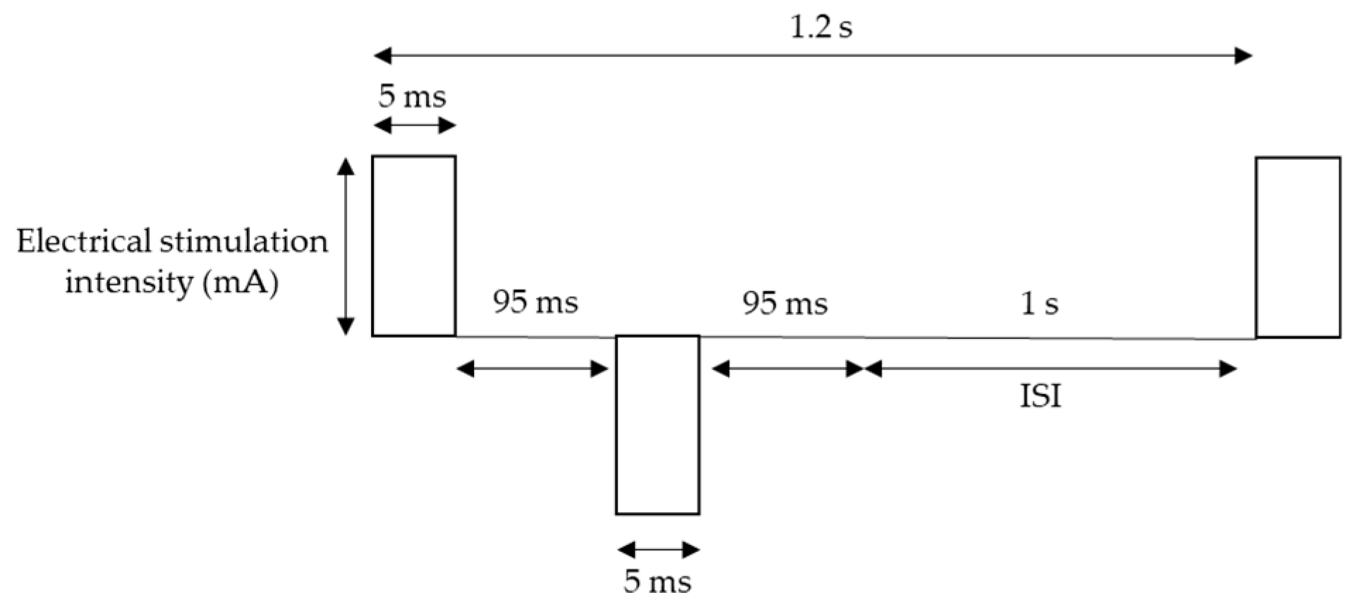
For pain stimulation, Electro-stimulator NS-101 (Unique Medical Co., Ltd., Tokyo, Japan) was used with Goldtrode
® disposable electrodes (Neurotron Co., Ltd., Baltimore, MD, USA). The diameter of electrode size was 1 cm. Electrical stimuli were delivered to the side of the right middle phalanx of the middle finger through the electrodes. The frequency of stimulation was 5 Hz, which is expected activate mostly one of the nociceptive afferent fibers: C-fibers, based on fMRI findings [
34], and square wave working on pain perception more than sine waveform [
35] was used. The other parameters of the waveform were 50 double pulses (bipolar square wave), pulse duration 5 ms, which optimizes for pain perception [
36], double pulse interval 95 ms, and inter-stimulus interval (ISI) 1 s [
35,
37] (
Figure 1). Each session contains 50 stimuli, and for each subject, two sessions were conducted with a 5-s pause between the two sessions, resulted in 100 trials, which lasted approximately 2 min in total.
EEG signals were recorded following the 10–20 system with 16 electrodes, namely Fp1, F3, T7, C3, P3, Pz, O1, Oz, O2, P4, C4, T8, F4, Fp2, Fz, and Cz. Ground electrodes were placed at CMS and DRL (based on Biosemi ActiveTwo, Amsterdam, Netherlands). The sampling rate and the bandwidth were 2048 Hz and 400 Hz, respectively. Subjects were asked to concentrate on the stimulation site and try to stay still with their eyes open.
In this study, we identified four perception levels: control (C), sensation (S), pain (P), and maximum pain (MP). All subjects received a test to determine their threshold for each perception level before the experiment. The threshold for C was identified by the least intensity of the stimulator, 0.1 mA, which could not cause any sensation. The threshold for S was identified as the least intensity that caused non-pain sensation, while the threshold for P was set for the minimal painful sensation or irritated feeling. Finally, the threshold for MP was determined as the highest intensity of pain that the subject could tolerate.
2.2. Preprocessing
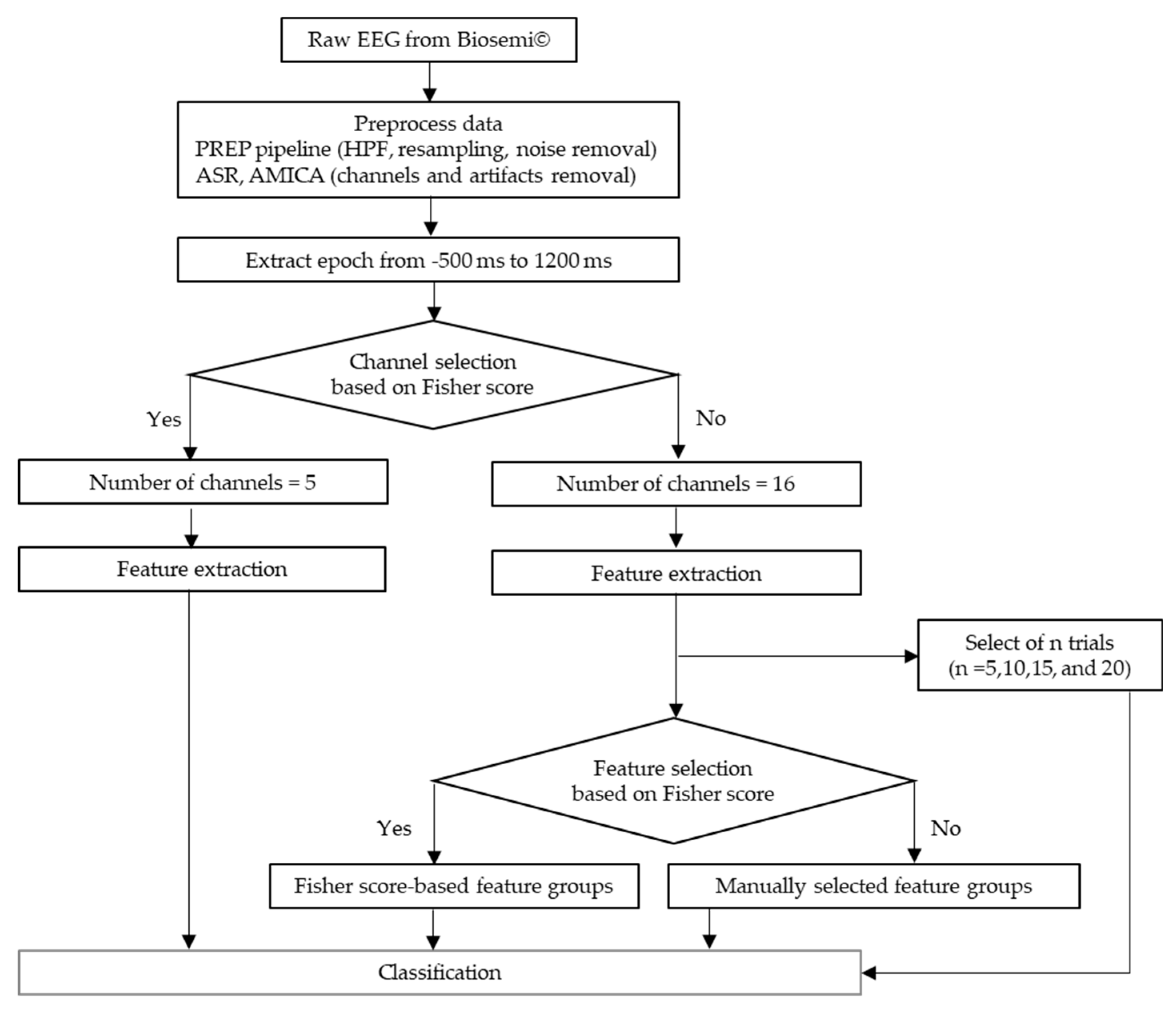
The flow of data preprocessing is shown in
Figure 2. The recorded EEG signals were preprocessed in Matlab 2017b (Mathworks, Natick, MA, USA) with EEGLAB toolbox [
38]. A preprocessing pipeline (PREP pipeline) [
39] was prepared for the EEG data to eliminate artifacts from power line frequency at 50 Hz and those that were physically-generated such as eye blinks or muscle movement. In the PREP pipeline, the EEG data were filtered using a high-pass filter at 1 Hz [
40] to remove baseline drift. Meanwhile, they were downsampled to 256 Hz. Moreover, Artifact Subspace Reconstruction (ASR) was used to clean continuous data by rejecting bad channels and removing high-variance artifacts [
41,
42]. All the removed channels were interpolated and the data were re-referenced to the average values of all ordinary channels. Furthermore, artifacts were removed by Adaptive Mixture Independent Component Analysis (AMICA) [
43,
44,
45], which performs ICA for mixing networks. Trial rejection was executed by removing the trials with the artifacts exceeding 5 times of standard-deviation. To avoid the bias possibly introduced by the initial startle responses, the first trial of every data was eliminated. Thus, we got the 435 data points that was aligned from 500 ms before to 1200 ms after stimulus onset for each trial.
Generally, usual ERP components could reflect a response to an external event but might not provide information about nonlinear brain activities, which could only be obtained with nonlinear analysis. Hence, we used channel selection for choosing channels with high pain perception related information. The effects of channel selection were investigated through the comparison between the classification of the pain-ERP data processed with and without the selection. Then the effects of feature selection, extraction and trial number on classification accuracy were investigated following the results of the channel selection.
2.3. Fisher Score-Based Channel Selection and Feature Selection
Due to the complexity of EEG, it is challenging to locate the EEG channels that brain’s responses with a higher signal-to-noise ratio, and less redundancy, so does the feature selection for EEG signals. A well-known criterion to resolve the channel and feature selection problem is Fisher score [
32,
33]. This information criterion is used to determine the most discriminative channels or features, and eliminate those noisy ones by selecting a subset of them, maximizing the distances between different classes (between-class distance) and minimizing the distance in one same class (within-class distance). The scatter matrices of within-class
and between-class
are calculated by Equations (1) and (2):
In the case of
c classes (
c = 4 for multiple-level scenarios in channel selection and feature selection),
ni indicates the training data samples in vector (
) for each class
i (
i = 1, …,
c). Note, for a certain class
i,
itself is actually a
ni-by-
nchannel_num matrix, where
nchannel_num is the number of EEG channels for further calculation, but for the simplicity of description,
is expressed as a
ni-dimensional vector. The prior probability of class
i is estimated by
.
denotes mean of training data of the
ith class,
is the mean vector of all samples, and
t stands for transpose matrix. Thus, the Fisher score of class separability for the
kth feature is calculated by:
where
Sb(
k) and
Sw(
k) are the
kth diagonal elements of
and
. Generally, the features with higher Fisher score are favored, while features with lower Fisher score, which are either irrelevant or noisy are to be discarded.
2.4. Feature Extraction
2.4.1. Higuchi’s Fractal Dimension (HFD)
FD is based on the self-similar behavior of time series [
27,
46], which can be used to assess the brain wave’s complexity [
28]. HFD estimates the complexity of the signals directly in time domain without reconstruction of any strange attractors. For time series of
N samples as
x(1),
x(2),
…,
x(
N) and
k are new time series.
k new signals are reconstructed as follows:
where
m and
k denote initial time point and the interval time, respectively, (
m = 1, 2, …,
k). Then, the length
Lm (
k) of each curve
is computed as:
where
is a normalizing factor for the
curve length. The average length of
m curves is estimated by:
The slope of a plot
log(
L(
k)) against
log(1/
k) is equal to FD, which can be calculated using the least-squares linear fitting. In this study
k = 217 was set, which comes from half of the number of data samples,
N, as explained in
Section 2.2 [
47]. Accordingly, the higher HFD value is, the higher EEG complexity is.
2.4.2. Grassberger-Procaccia (GP) Correlation Dimension
In the area of EEG stochastic analysis, dimension measurements are widely used to discriminate between a nonlinear deterministic or noise derived time series. GP [
26,
29,
30,
48] is also known as one of the FD criteria which evaluates the correlation dimension,
D2, of a chaotic attractor in the phase space dimension. Given a time series of data
xi, which is the
ith data of EEG amplitude, while
M is the embedding dimension with the time delay,
Then,
xj is the reconstructed phase space vector. For the
M-dimensional reconstructed phase space, the correlation function is calculated as follows:
where
is the Euclidean distance between the vector of data
xi and
xj.
H(
x) is the Heaviside step function, which is defined as
H(
x) = 0 for
x ≤ 0, otherwise
H(
x) = 1 for
x > 0. A small value of the separation distance of the vectors is denoted as
r. The multiplier
is added to normalize the pairs of points on the attractor. The correlation dimension,
D2, is computed as:
GP is a slope of the straight line of plot log(C(r)) versus log(r) at a given value, M = 12 in this study, which is the M-value that led GP to saturation.
2.4.3. Auto Correlation Function
Auto-correlation function (ACF) is a measurement of the correlation between values of itself at different time steps [
49]. This method is often used in time domain signal analyzing to find the patterns or randomness in the data. For a time sequence
x(1),
x(2), …,
x(
N), at lag
k (
k = 0, 1, …), its auto-covariance coefficient could be determined as follows:
where
is the variance of the time series. Then, the autocorrelation function is:
where the lag
k = 4 and 15, significant changes at for data with channel selection and without channel selection, respectively. In this study, the ACF was calculated over EEG channels, that is,
N = 5 and 16, for the case with and without channel selection, respectively.
2.4.4. Moving Variance
Moving variance (VAR) is used to measure statistics of streaming signals by computing the mean in one pass over the data and calculating the square of the differences from mean as a second pass afterward [
50]. Each variance,
V, is assessed over five sliding window lengths across each EEG channel in this study. For each sample
x(1),
x(2), …,
x(
N), the variance is defined as:
Again, the VAR was calculated over EEG channels, that is, N = 5 and 16, for the case with and without channel selection, respectively.
2.5. Feature Selection and Feature Grouping
We used a series of 435 time points from pain-ERP, which were averaged over all trials to extract features for each subject, as shown in
Figure 3 both HFD and GP were calculated for each channel for the same length of pain-ERP signals, then, extracted further by ACF and VAR. All obtained values were named according to their extraction methods and functions as “HFD”, “HFD_ACF”, and “HFD_VAR” for features with Higuchi’s method, Higuchi’s with autocorrelation, and Higuchi’s with moving variance, respectively. Also, specifying the same idea to the correlation dimension method by giving the name “GP”. Then, we had six features with Fisher score-based channel selection and other 6 features without Fisher score-based channel selection. For each type of feature, from the data of each channel, one feature value was calculated. That is, for the case with and without channel selection, the feature vector is 5-dimensional and 16 dimensional, respectively.
According to
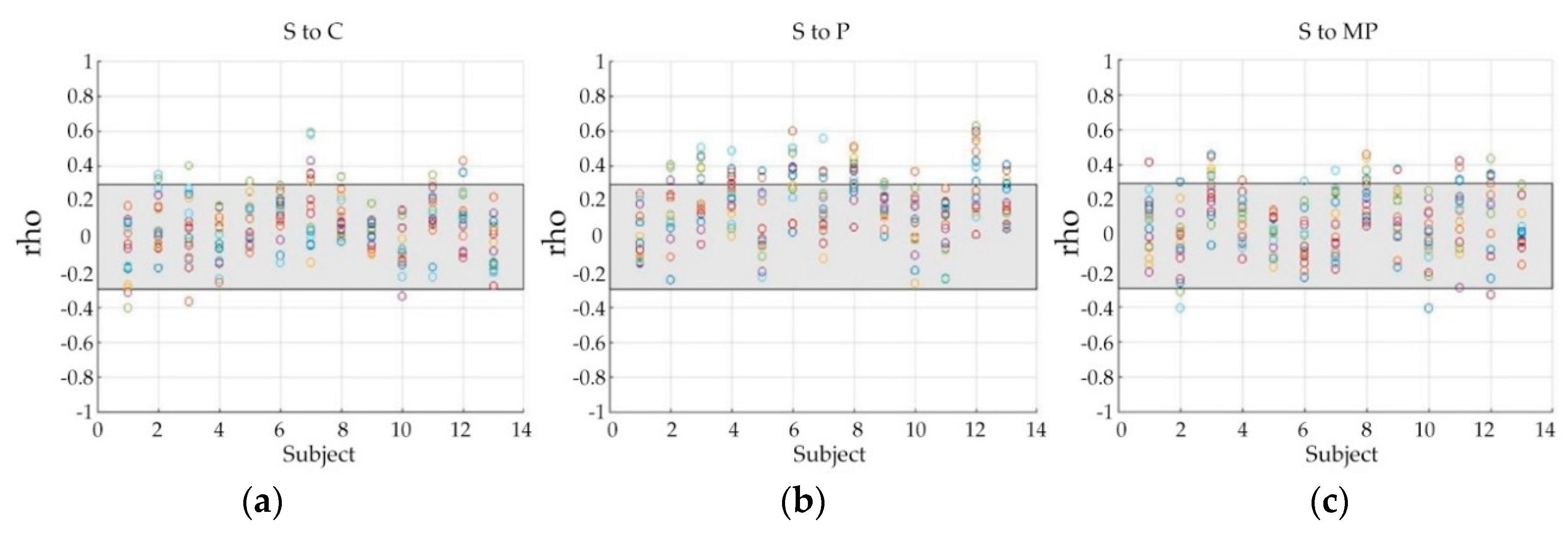
Figure 3, there might be some perception levels that are non-discriminative or less-discriminative to all the features for multiple classifications. Thus, we used Spearman’s correlation coefficients (rho) to investigate the correlation between data of different pain perception levels, displayed in
Figure 4, in which, each color circle indicates the correlation between the data of a specific channel, and the grey area shows the weak correlation zone bounded by 0.3 and −0.3. A correlation ratio of the number of points located outside of the grey zone to that of points located inside the grey zone was used to measure how the data are strongly correlated to each other. Compared with ‘S to C’ and ‘S to MP’ correlation, ‘S to P’ showed a comparatively higher ratio (0.10 of ‘S to C’, 0.15 of ‘S to MP’, and 0.27 of ‘S to P’). The correlation ratio value of ‘S to P’ (0.27) is much higher than the other pairs (0.07 of both ‘C to P’ and ‘C to MP’), and higher than that of ‘P to MP’, which has a ratio of 0.21.
For each binary classification, 26 samples were obtained. For multiple-level classifications, we collected 52 samples and 39 samples for four-level (C, S, P, and MP) and three-level classification (excluding S), respectively. We used Matlab’s neural pattern recognition application for classifying EEG features. All samples were split into 75% for training, 10% for validation, and 15% for testing. The results with cross validation and without cross validation will be compared. We assigned ten neurons for weighting inputs in the only hidden layer of the network.
Furthermore, to find the best features for multiple-level classifications, we compared FD-based features of pain-ERP with the statistic features, which are used in previous studies for classifying cognitive skills [
51]. All the statistical and FD-based features were processed to calculate their Fisher score. After that, feature groups were formed according to the ranks of the score.
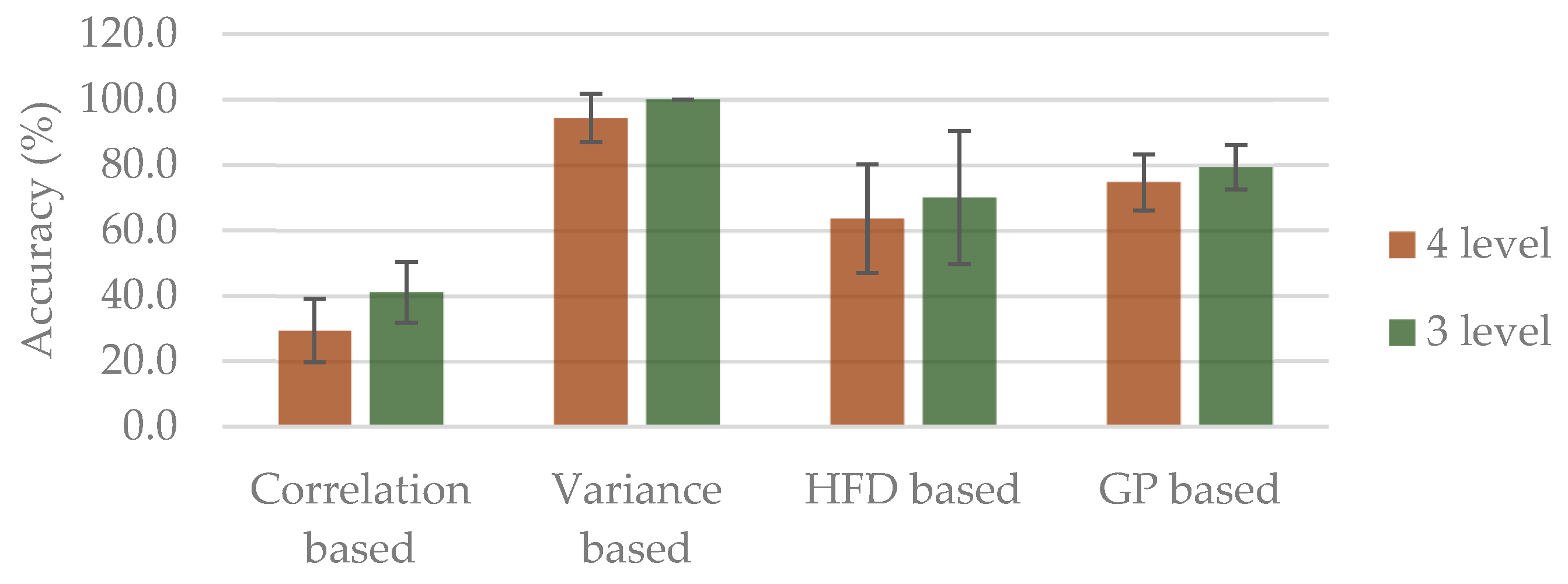
Moreover, in order to further investigate the role of FD-based features, several feature groups were designated based on the following aspects of the features:
- (1)
Correlation-based (HFD, HFD_ACF, GP_ACF)
- (2)
Variance-based (GP, HFD_VAR, GP_VAR)
- (3)
HFD-based (HFD, HFD_ACF, HFD_VAR)
- (4)
GP-based (GP, GP_ACF, GP_VAR)
5. Conclusions
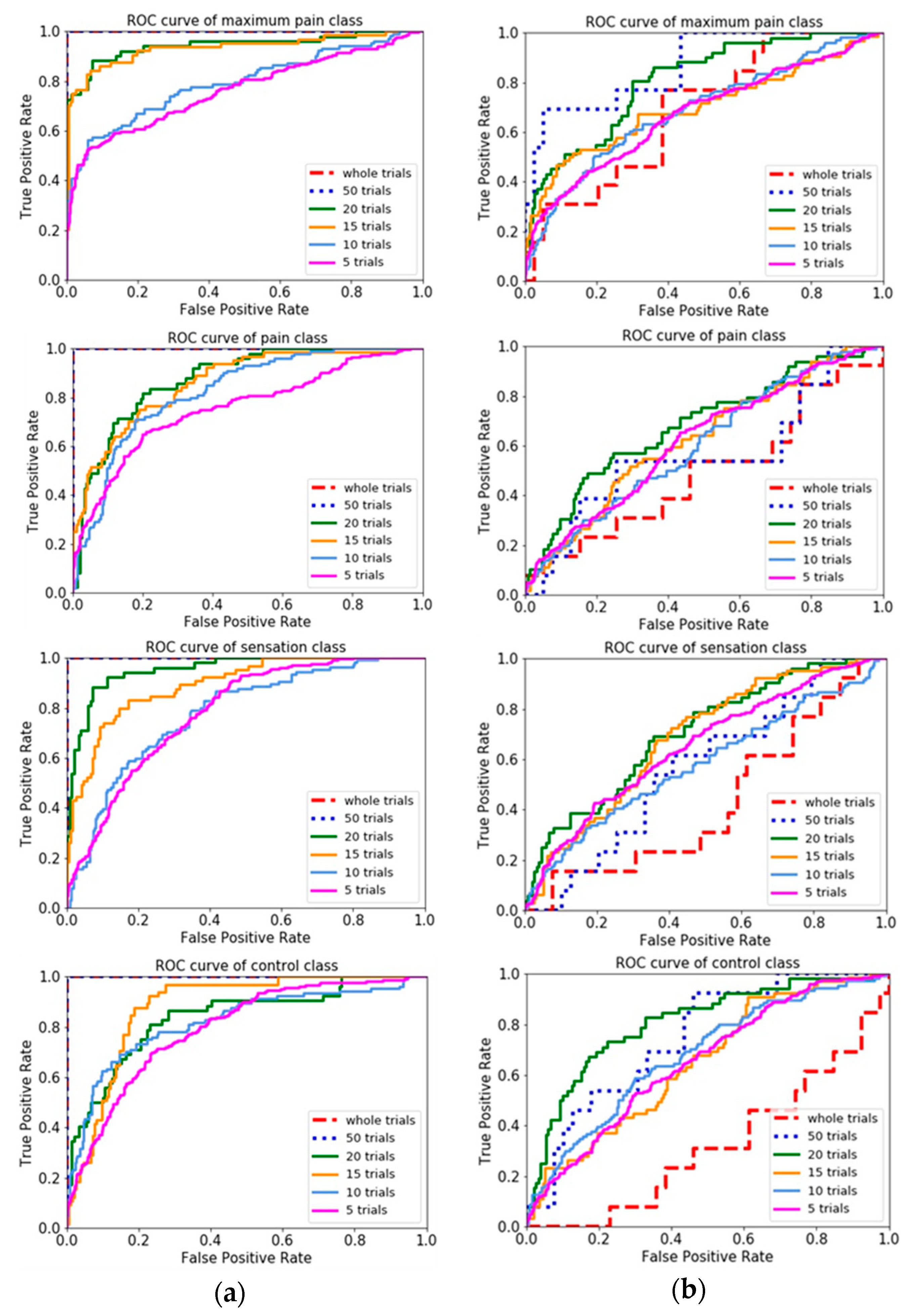
In this study, nonlinear feature extraction based on pain-ERP for the prediction of different pain perception thresholds is proposed. Epoched EEG in time domain was selected to extract a set of 6 features, then used for classifications by an artificial neural network structure. Our results showed that the proposed use of GP with VAR is superior to other features for two-level classification, and also achieved the highest accuracy for three-level classification (without sensation condition). Channel selection by Fisher score in this study has an insignificant difference of 0.49, 0.25, and 0.91 for four, three, and two-level from without channel selection based on Fisher score. Based on the results of combined FD-based features, a variance based group has the best accuracies of 87.5% and 100% for four-level and three-level classification without channel selection, respectively, which is also better than combined statistical features. Moreover, averaging of the n-trial was analyzed to examine the tendency of real-time, which showed that having more trials of EEG has better performance due to having higher amount of data points to calculate. Through this study, evidence has been shown that using nonlinear features based on pain-ERP can classify pain perception levels from non-invasive electrical stimulation. Furthermore, we believe our findings can be applied in the field of rehabilitation and neurosciences for objective pain assessment.


