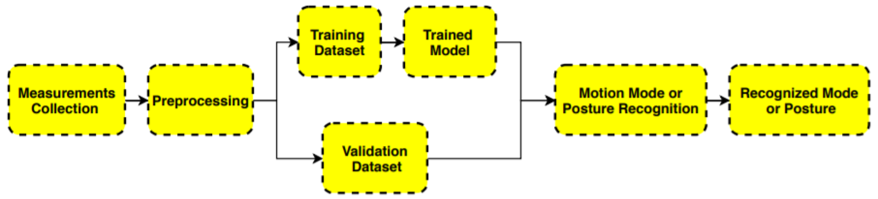
Figure 1.
Procedure of recognition.
Figure 1.
Procedure of recognition.
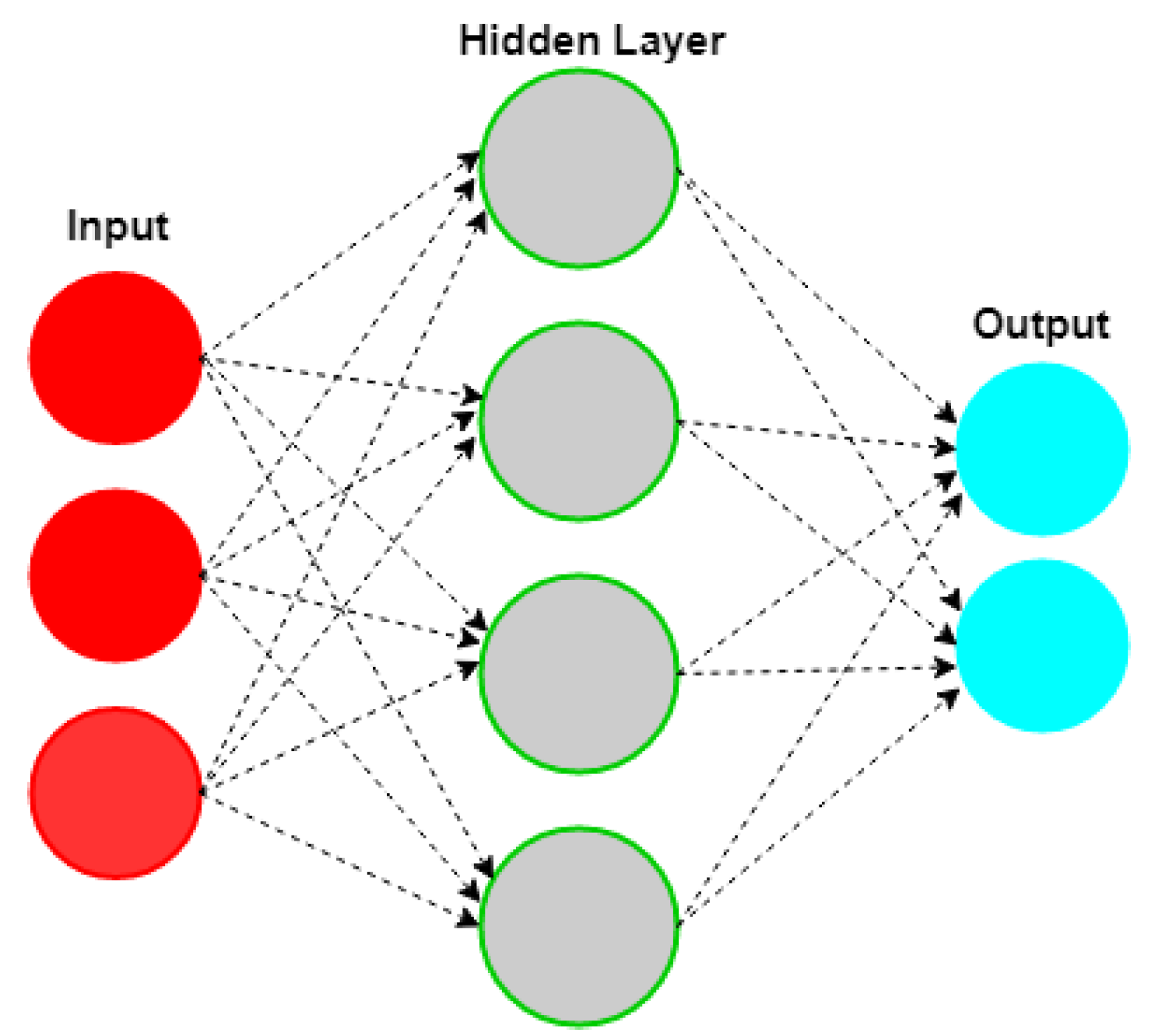
Figure 2.
Structure of ANN.
Figure 2.
Structure of ANN.
Figure 3.
Training and test situation by raw dataset.
Figure 3.
Training and test situation by raw dataset.
Figure 4.
Filtered MEMS measurements.
Figure 4.
Filtered MEMS measurements.
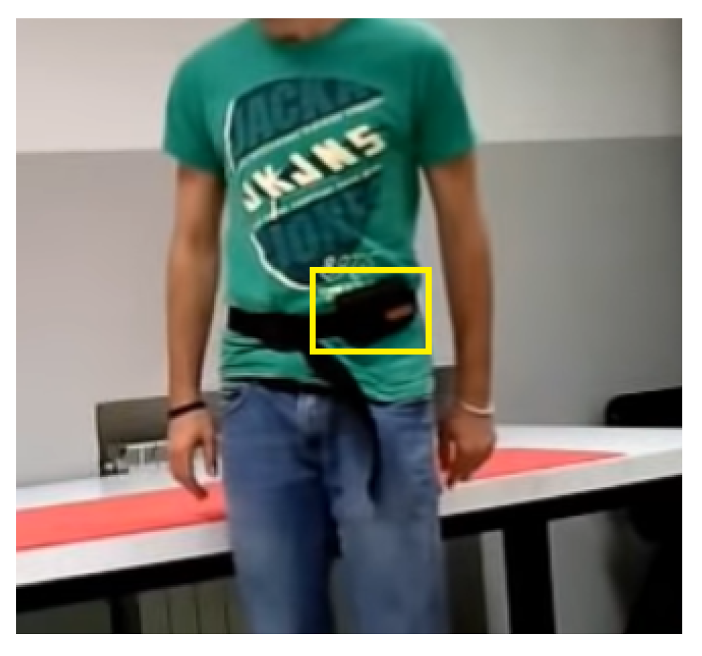
Figure 5.
Pedestrian taking the test with smartphone on waist.
Figure 5.
Pedestrian taking the test with smartphone on waist.
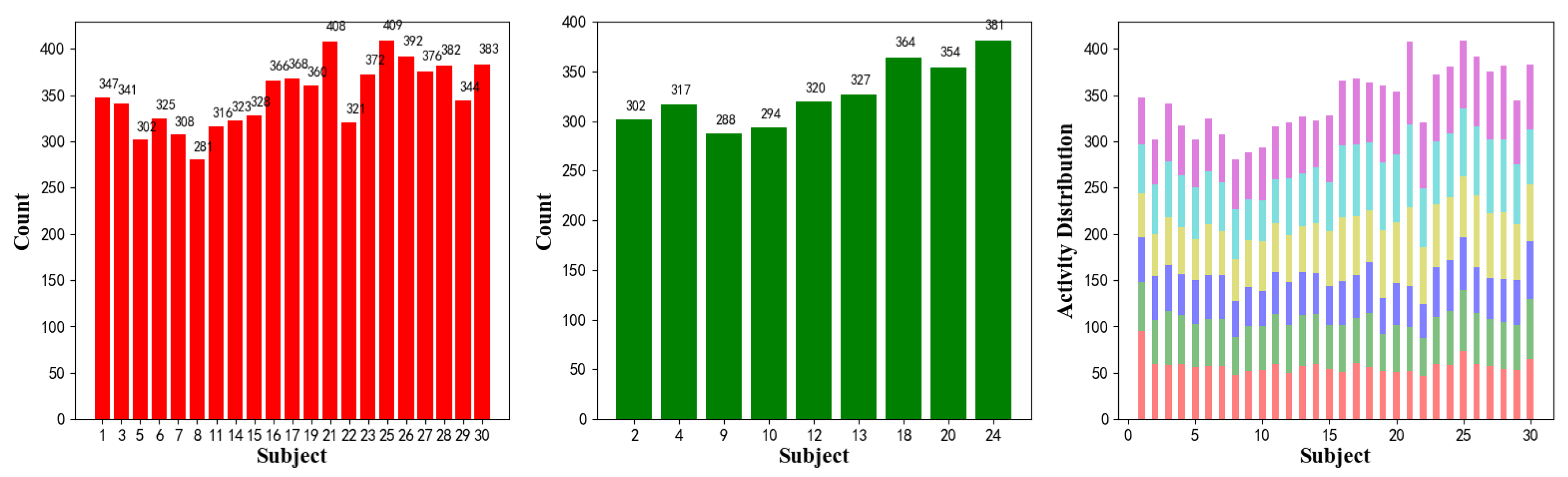
Figure 6.
Human activity recognition dataset of UCI. Left: activity distributions of training data and related subjects; Middle: dataset distribution of validation data; Right: six activities’ distribution of 30 subjects.
Figure 6.
Human activity recognition dataset of UCI. Left: activity distributions of training data and related subjects; Middle: dataset distribution of validation data; Right: six activities’ distribution of 30 subjects.
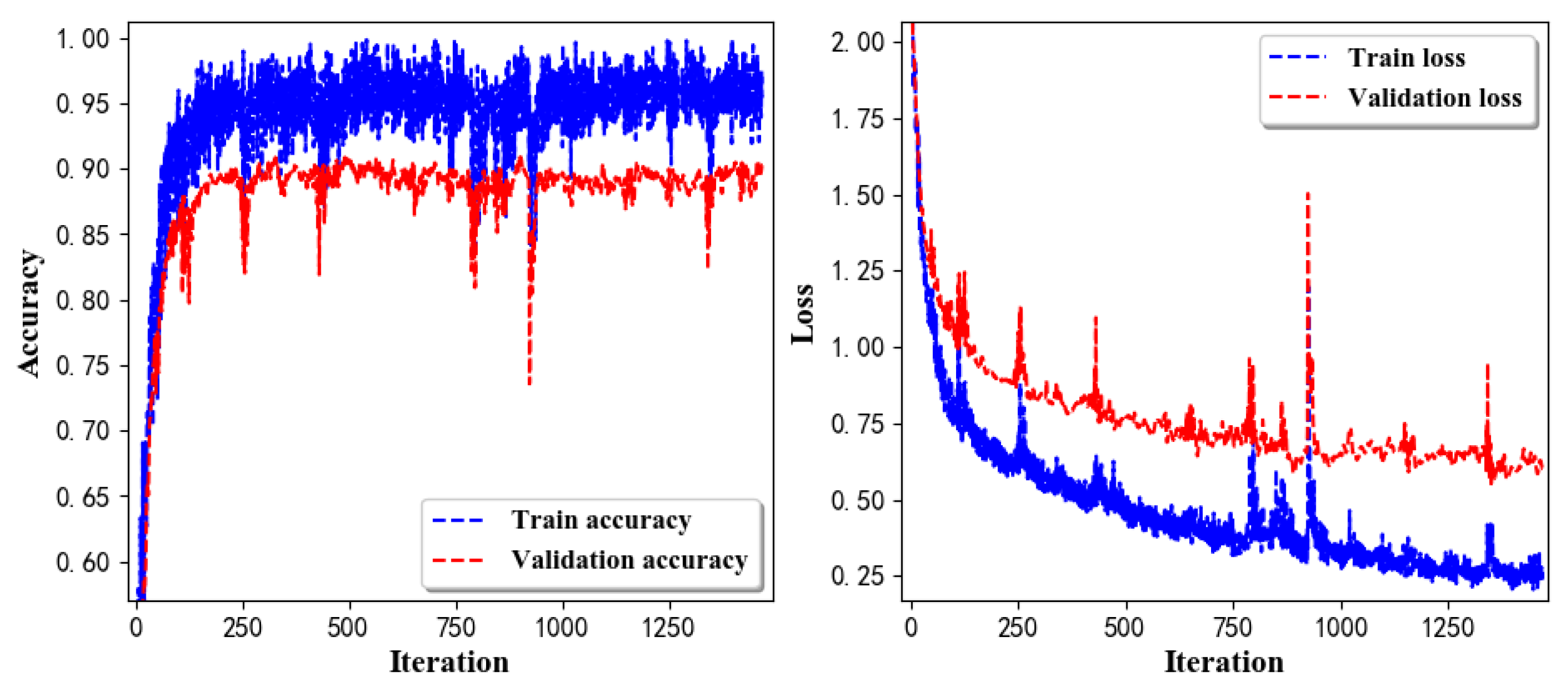
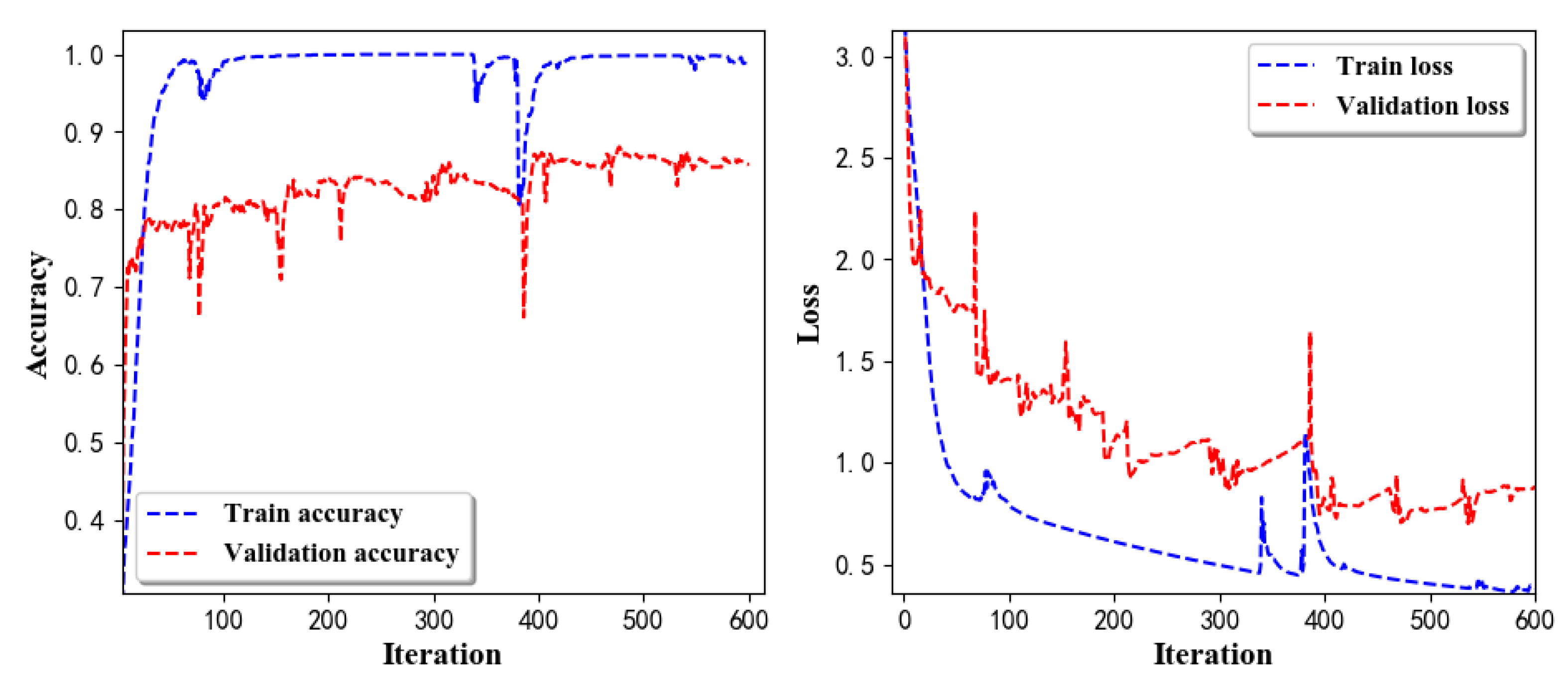
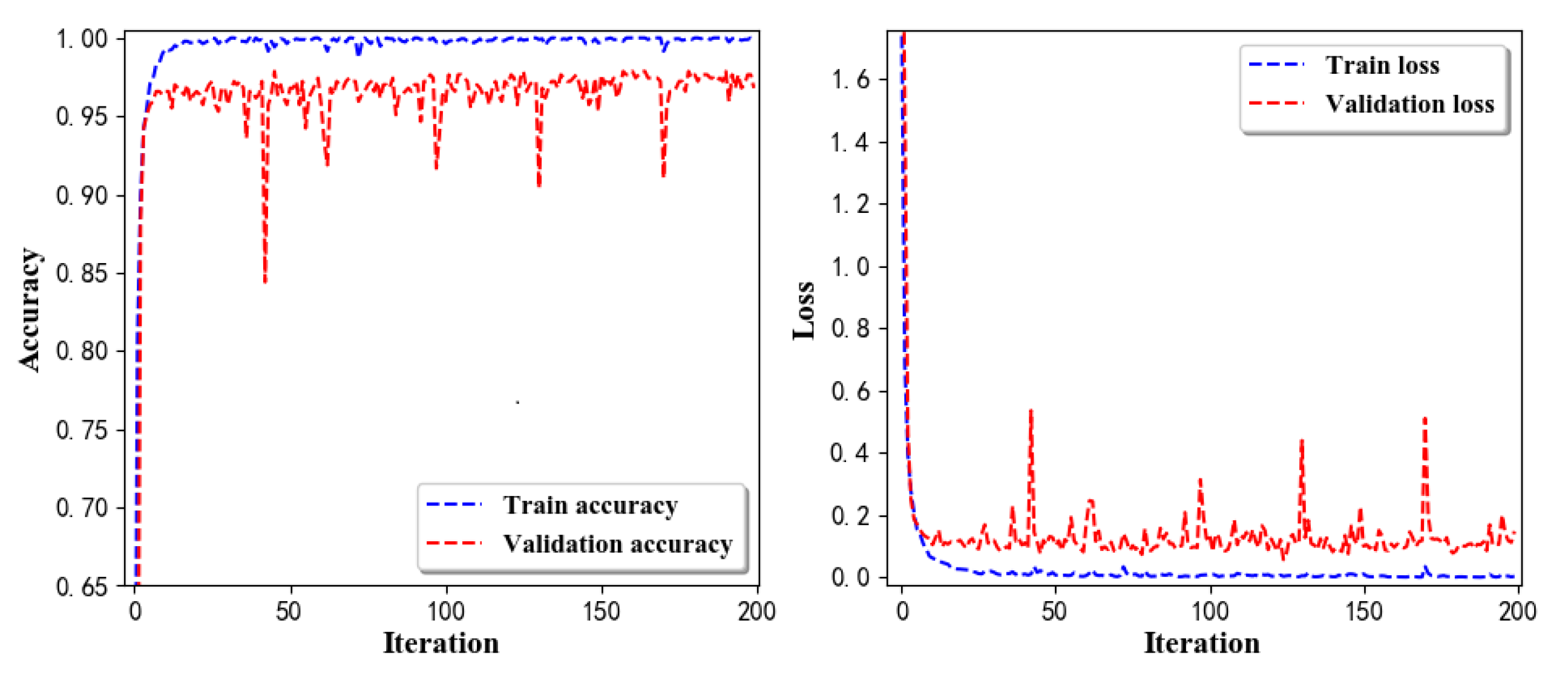
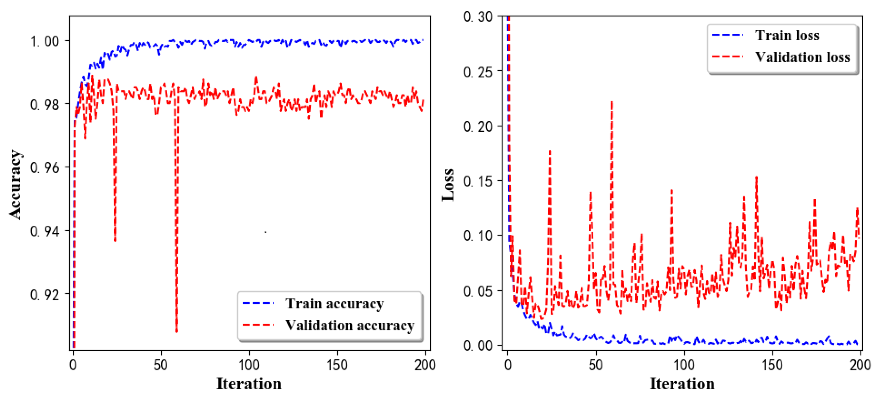
Figure 7.
Accuracy (left) and loss (right) information of training and validation procedure.
Figure 7.
Accuracy (left) and loss (right) information of training and validation procedure.
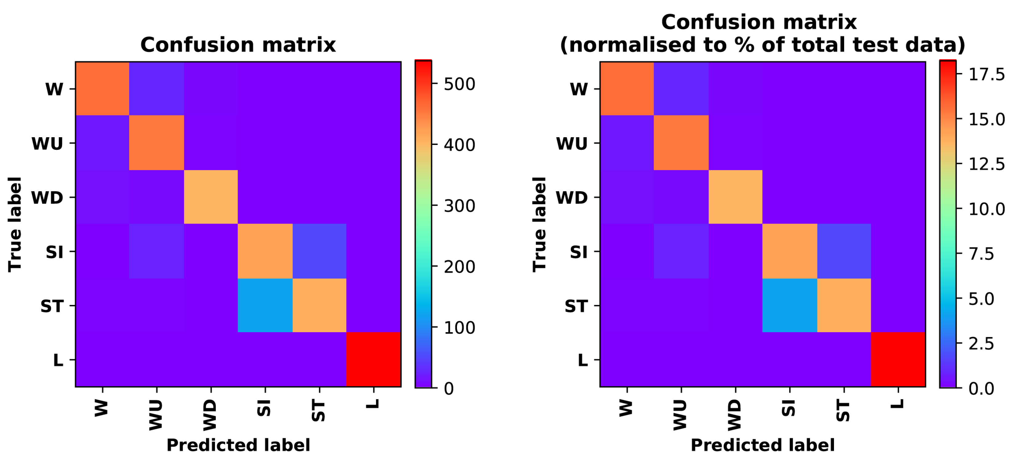
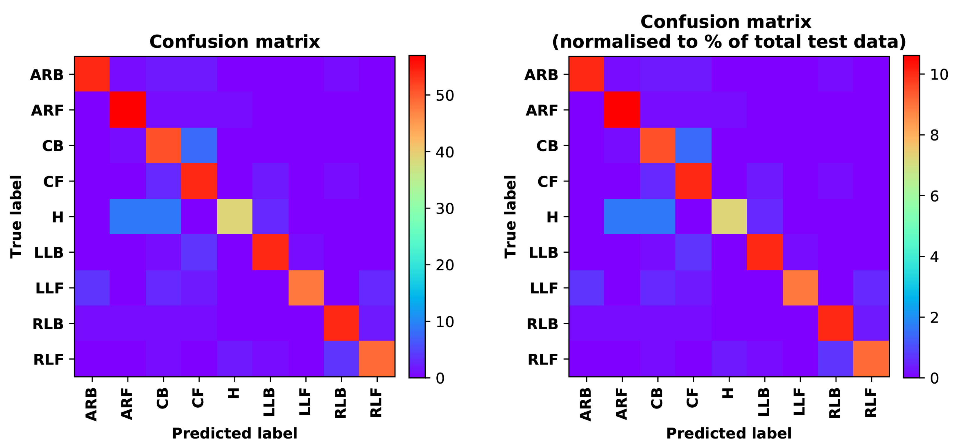
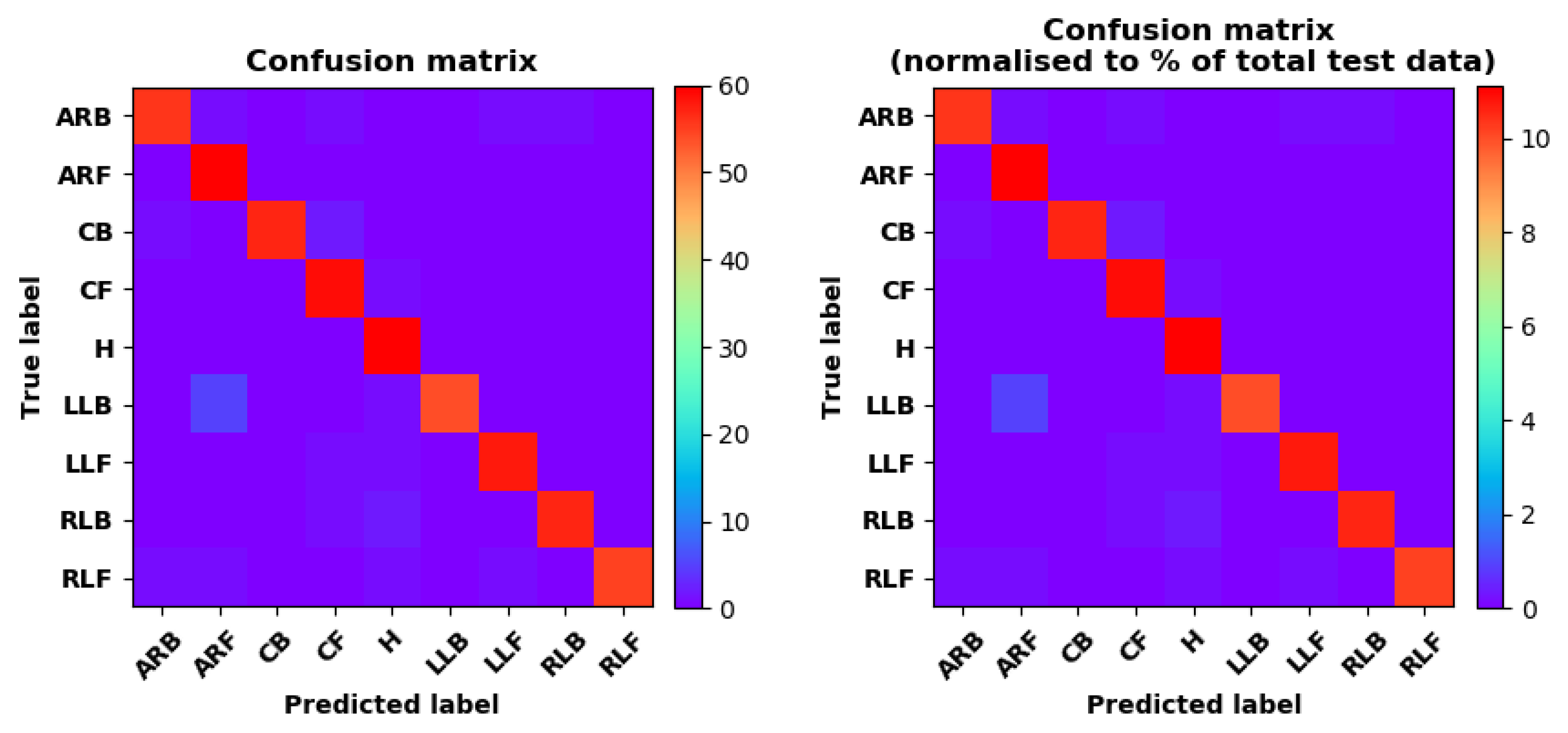
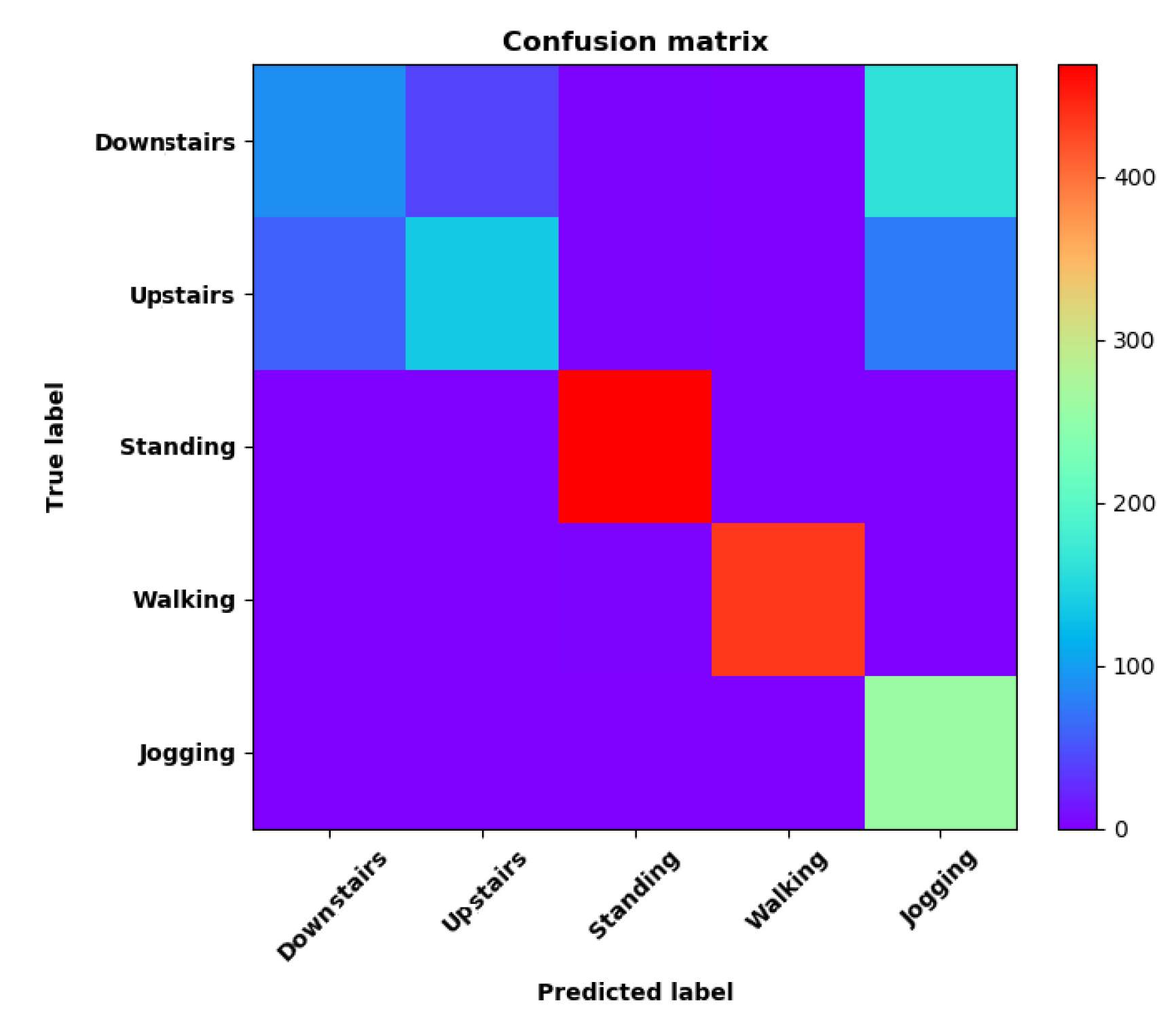
Figure 8.
left graph is the confusion matrix of classification test using the model trained by LSTM network; right is the normalised confusion matrix.
Figure 8.
left graph is the confusion matrix of classification test using the model trained by LSTM network; right is the normalised confusion matrix.
Figure 9.
Accuracy (left) and loss (right) information of training and validation procedure.
Figure 9.
Accuracy (left) and loss (right) information of training and validation procedure.
Figure 10.
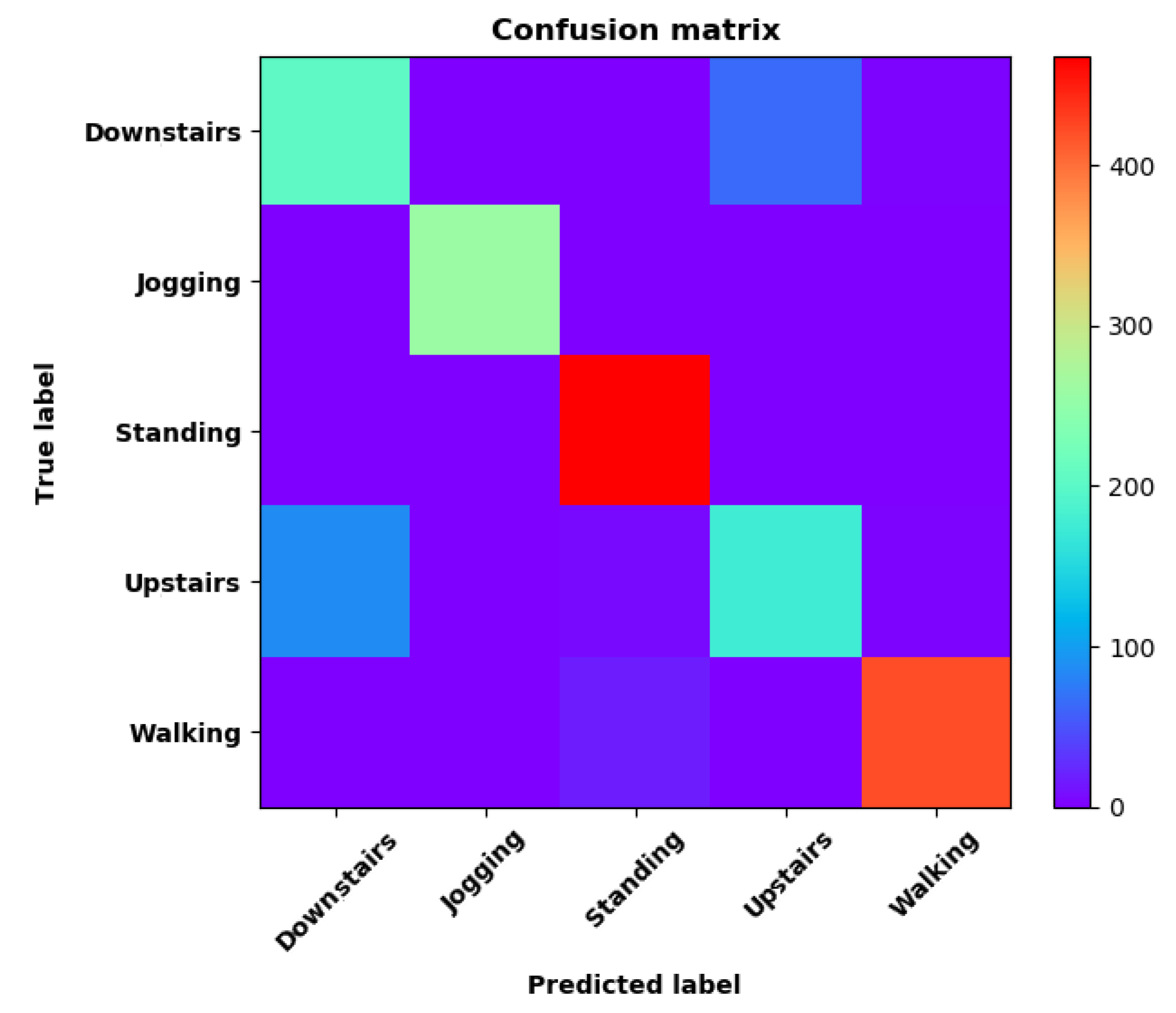
left graph is the confusion matrix of classification test using the model trained by CNN network; right is the normalised confusion matrix.
Figure 10.
left graph is the confusion matrix of classification test using the model trained by CNN network; right is the normalised confusion matrix.
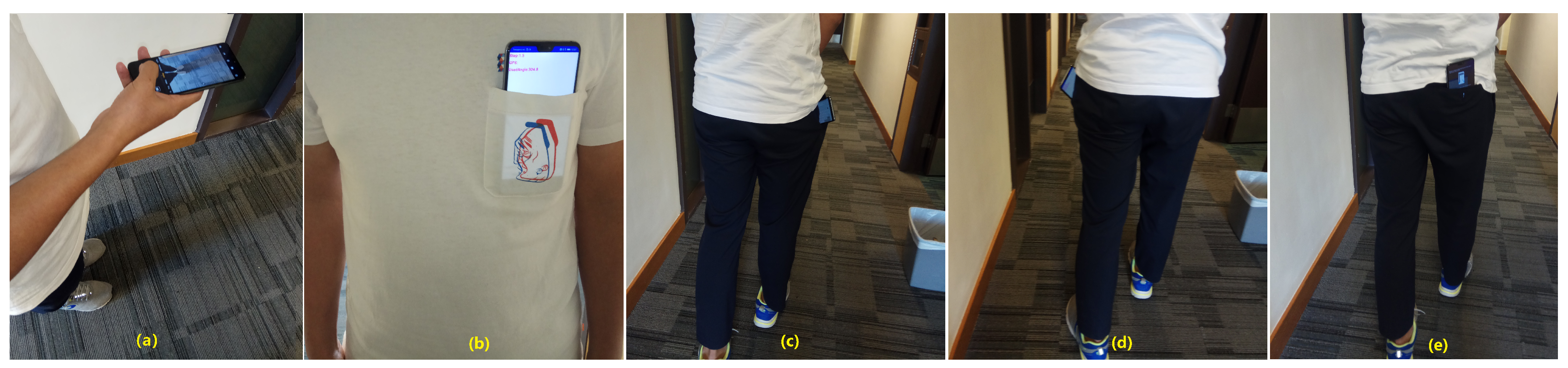
Figure 11.
Smartphone posture recognition experiment. (a) is holding smartphone; (b) is in the chest pocket; (c) is in the right trouser pocket; (d) is in the left trouser pocket; (e) is in the buttock pocket
Figure 11.
Smartphone posture recognition experiment. (a) is holding smartphone; (b) is in the chest pocket; (c) is in the right trouser pocket; (d) is in the left trouser pocket; (e) is in the buttock pocket
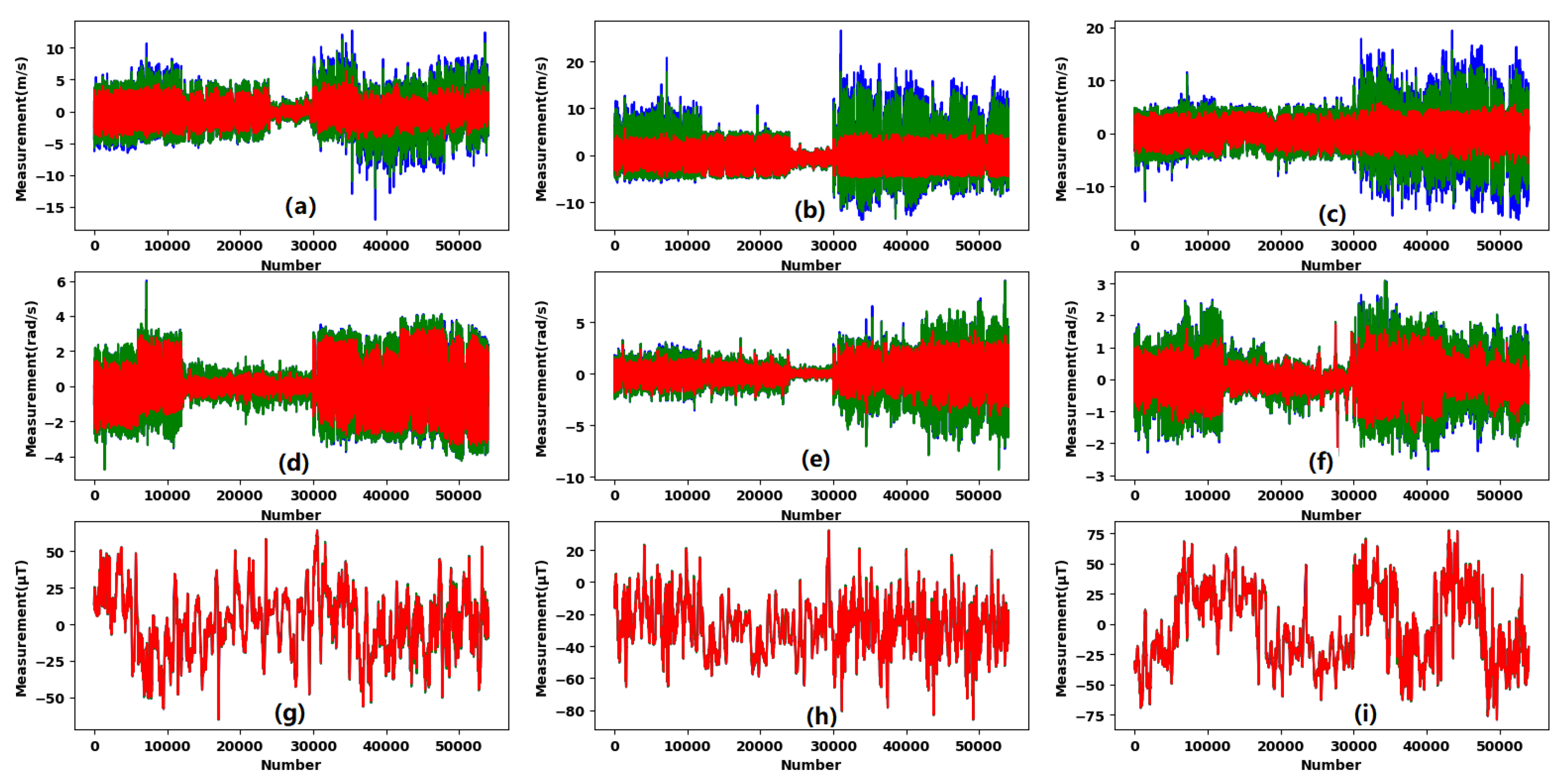
Figure 12.
MEMS measurement processing strategies; (a)–(c) are filtered accelerometer x-, y-, z-axis measurements; (d)–(f) are filtered gyroscope x-, y-, z-axis measurements; (g)–(i) are filtered magnetometer x-, y-, z-axis measurements.
Figure 12.
MEMS measurement processing strategies; (a)–(c) are filtered accelerometer x-, y-, z-axis measurements; (d)–(f) are filtered gyroscope x-, y-, z-axis measurements; (g)–(i) are filtered magnetometer x-, y-, z-axis measurements.
Figure 13.
Accuracy (left) and loss (right) information of training and validation procedure.
Figure 13.
Accuracy (left) and loss (right) information of training and validation procedure.
Figure 14.
left graph is the confusion matrix of classification test using the model trained by LSTM network; right is the normalised confusion matrix.
Figure 14.
left graph is the confusion matrix of classification test using the model trained by LSTM network; right is the normalised confusion matrix.
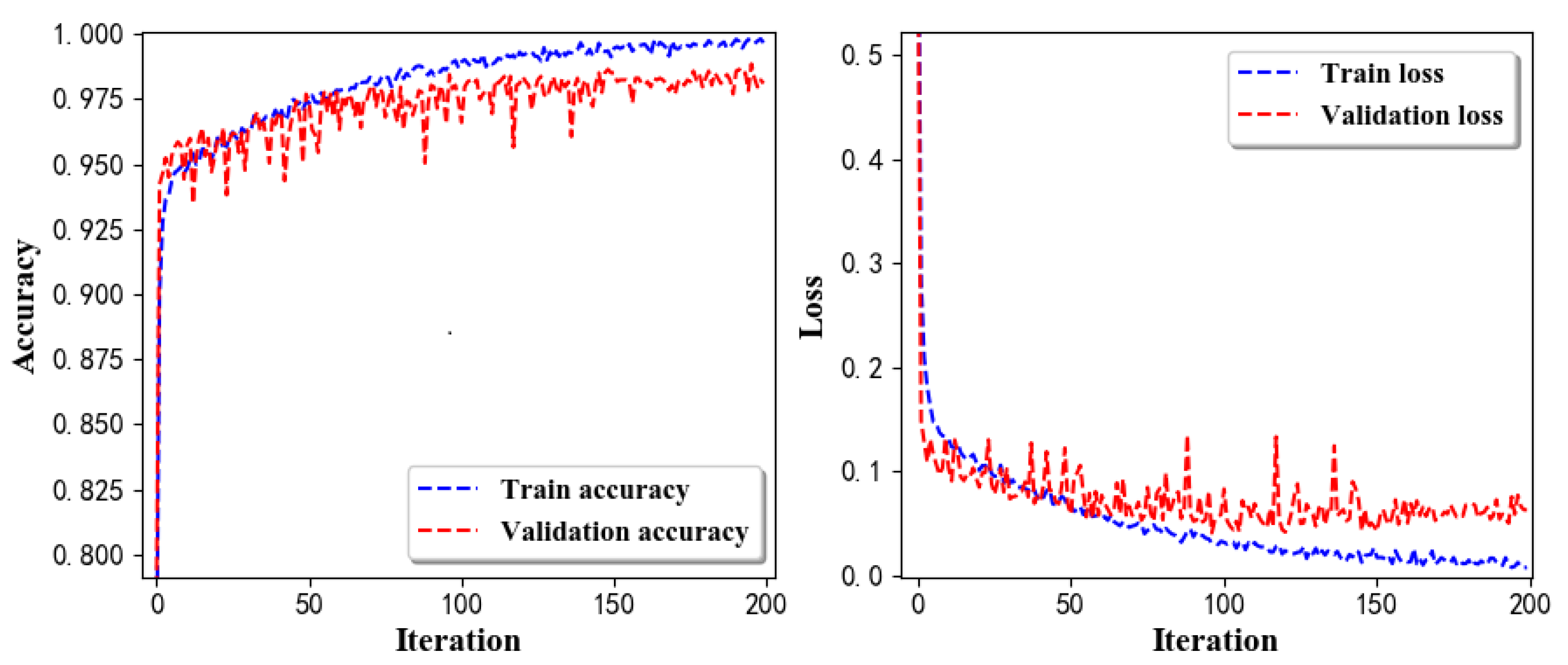
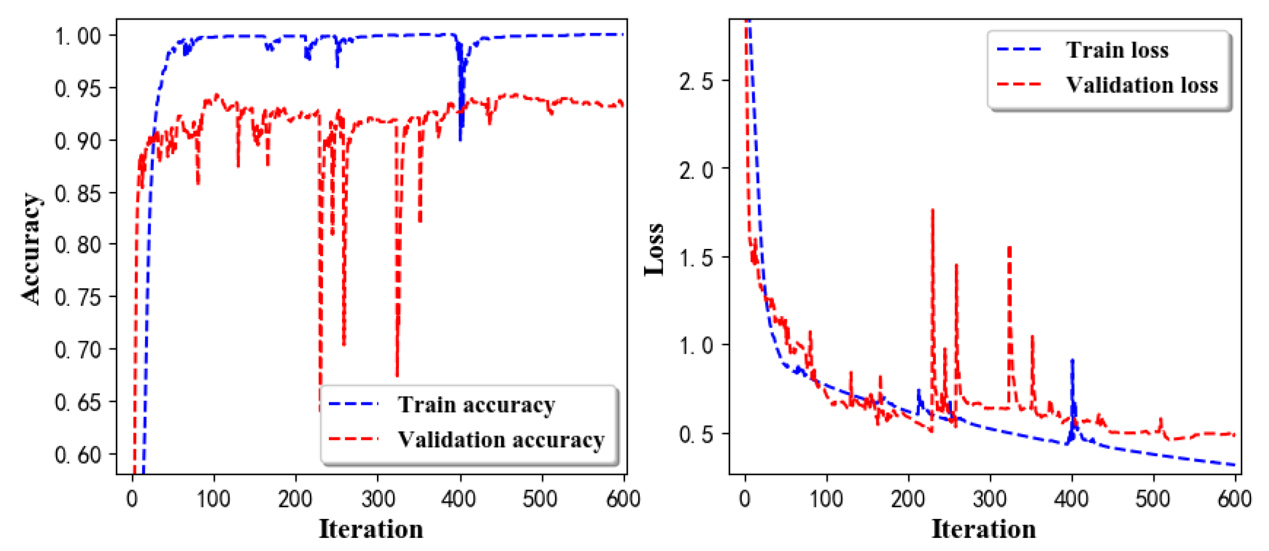
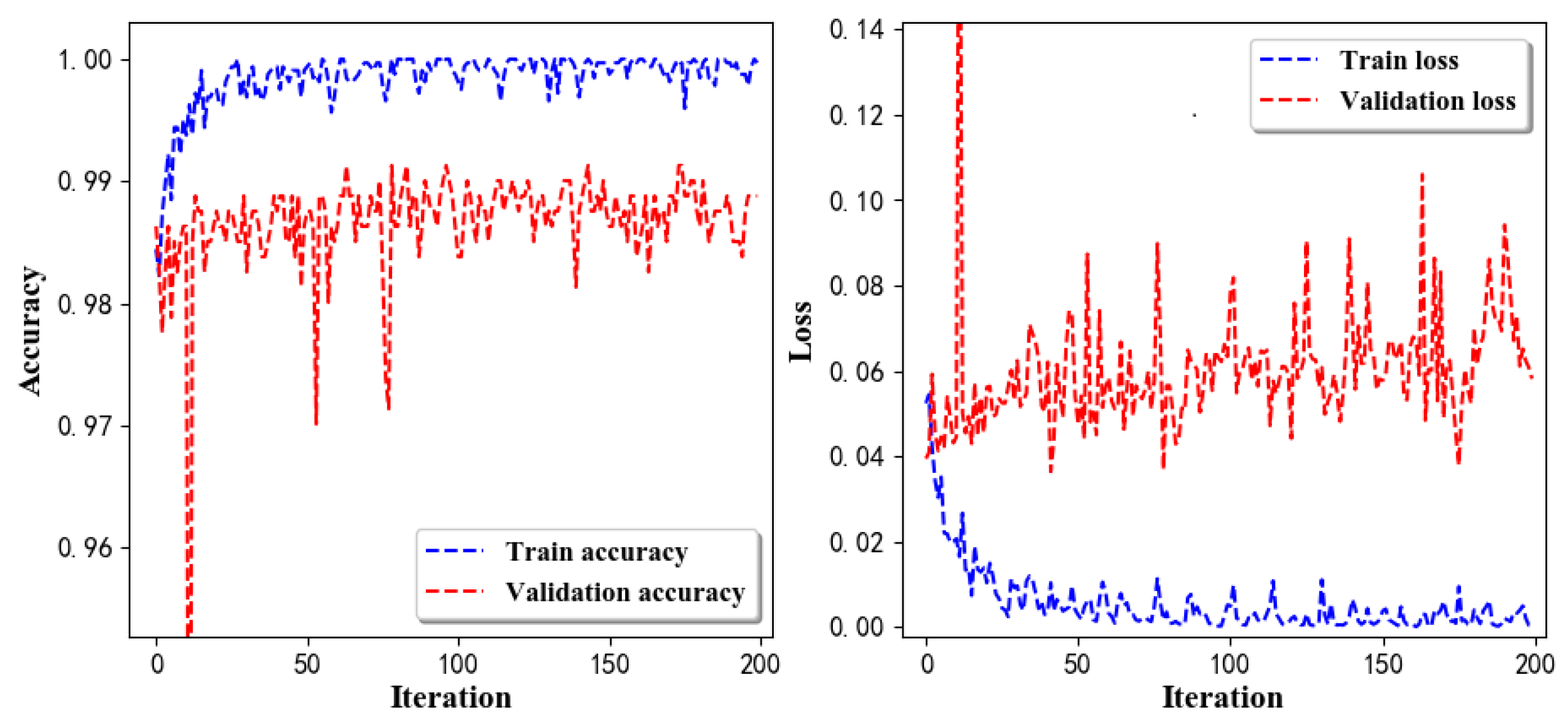
Figure 15.
Accuracy (left) and loss (right) of training and validation procedure using filtered measurements.
Figure 15.
Accuracy (left) and loss (right) of training and validation procedure using filtered measurements.
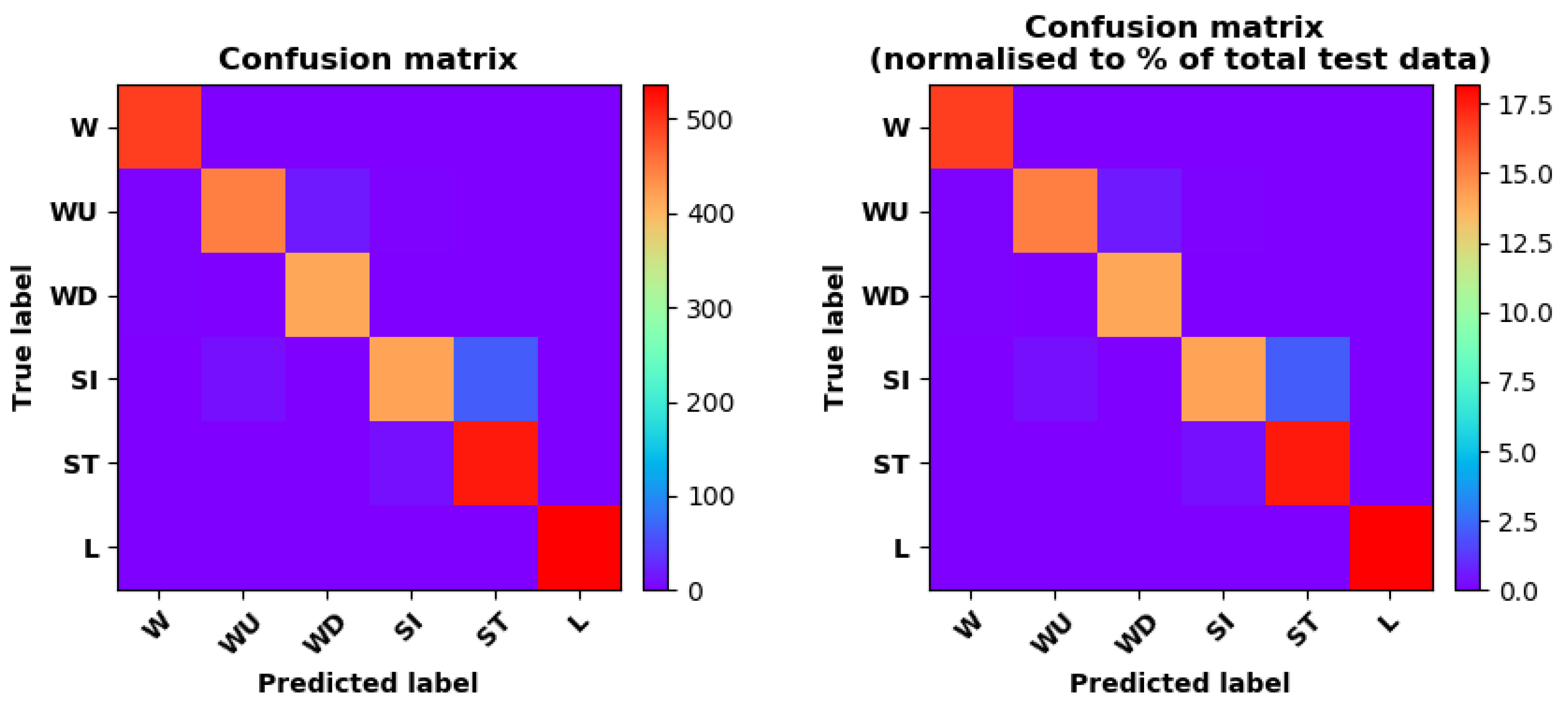
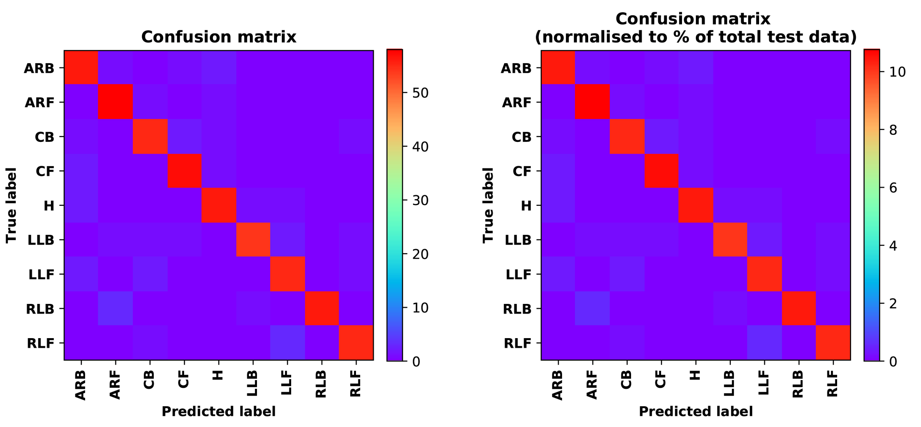
Figure 16.
left graph is the confusion matrix of classification test using the model trained by LSTM network with filtered measurements; right is the normalised confusion matrix.
Figure 16.
left graph is the confusion matrix of classification test using the model trained by LSTM network with filtered measurements; right is the normalised confusion matrix.
Figure 17.
Accuracy (left) and loss (right) information of training and validation procedure.
Figure 17.
Accuracy (left) and loss (right) information of training and validation procedure.
Figure 18.
left graph is the confusion matrix of classification test using the model trained by CNN network; right is the normalised confusion matrix.
Figure 18.
left graph is the confusion matrix of classification test using the model trained by CNN network; right is the normalised confusion matrix.
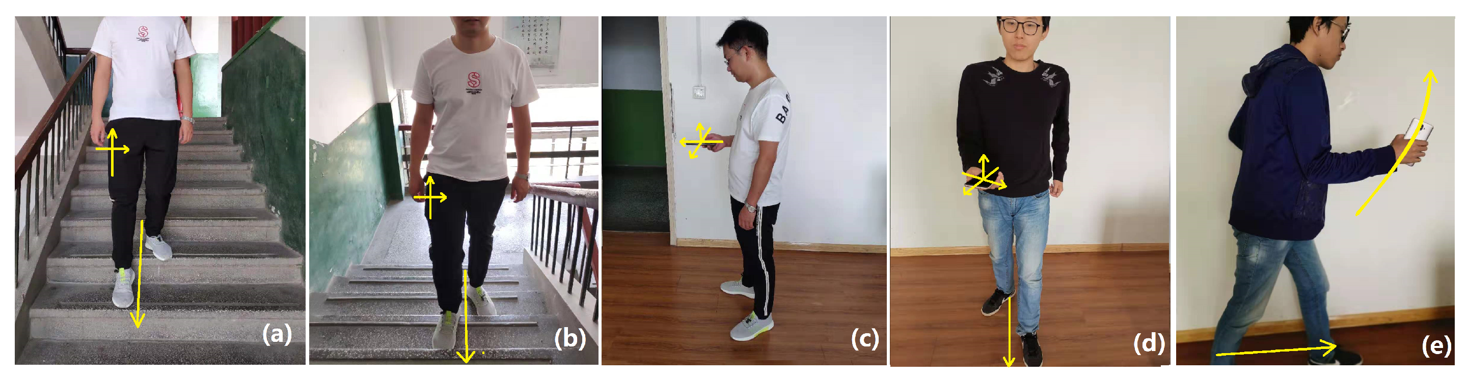
Figure 19.
Real-time recognition test of comprehensive pedestrian activities.(a) is downstairs; (b) is upstairs; (c) is standing; (d) is walking; (e) is jogging.
Figure 19.
Real-time recognition test of comprehensive pedestrian activities.(a) is downstairs; (b) is upstairs; (c) is standing; (d) is walking; (e) is jogging.
Figure 20.
Accuracy (left) and loss (right) information of training and validation procedure.
Figure 20.
Accuracy (left) and loss (right) information of training and validation procedure.
Figure 21.
Confusion matrix of classification test using the model trained by CNN network.
Figure 21.
Confusion matrix of classification test using the model trained by CNN network.
Figure 22.
Accuracy (left) and loss (right) information of training and validation procedure with light measurements.
Figure 22.
Accuracy (left) and loss (right) information of training and validation procedure with light measurements.
Figure 23.
Confusion matrix of classification test using the model trained by CNN network with light measurements.
Figure 23.
Confusion matrix of classification test using the model trained by CNN network with light measurements.
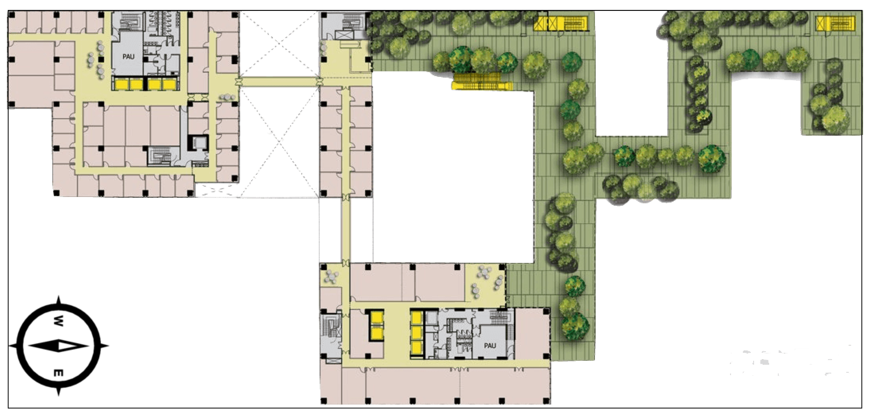
Figure 24.
The plan of test field.
Figure 24.
The plan of test field.
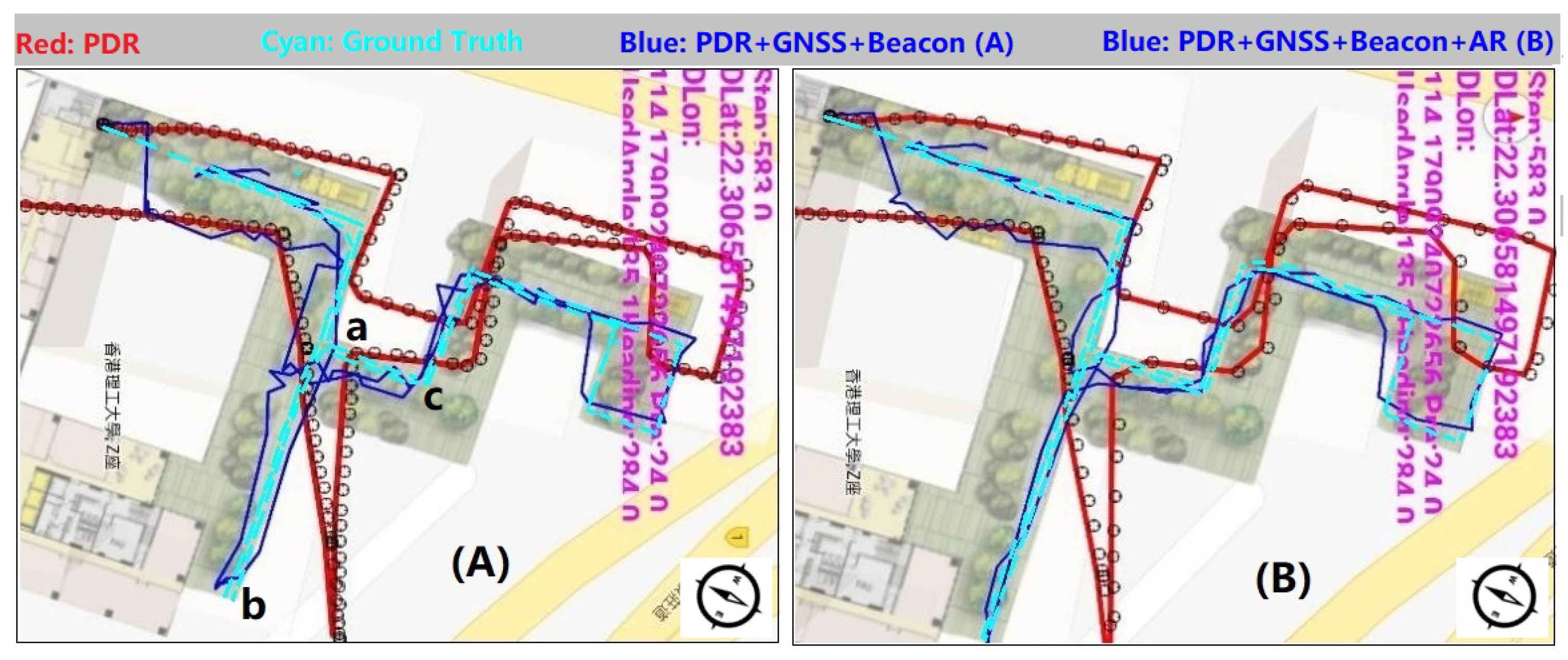
Figure 25.
Graph (A) is the navigation test result without AR(Activity Recognition); (B) uses AR.
Figure 25.
Graph (A) is the navigation test result without AR(Activity Recognition); (B) uses AR.
Table 1.
Features extracted from measurements.
Table 1.
Features extracted from measurements.
| Category | Type | Definition |
|---|
| Statistical | Mean | |
| | Median | |
| | Root Mean Square | |
| | 75th percentile | percentile , |
| | Variance | |
| | Standard Deviation | |
| | Skewness | |
| | Binned Distribution | bindstbn |
| | Mean Absolute Deviation | |
| Frequency Domain | Fourier Transform | |
| | Short-Time Fourier Transform | |
| | Discrete Cosine Transform | |
| | Continuous Wavelet Transform | |
| | Discrete Wavelet Transform | |
| | Wigner Distribution | |
| | Frequency Domain Entropy | |
| Energy, Power, Magnitude | Energy | energy |
| | Sub-band Energies | energy |
| | Sub-band Energy Ratios | subband energy |
| | Signal Magnitude Area | |
| Time Domain | Zero-Crossing Rate | |
Table 2.
Template of a confusion matrix for a four-class classifier.
Table 2.
Template of a confusion matrix for a four-class classifier.
| Actual Mode | Predicted Mode |
|---|
| Class 1 | Class 2 | Class 3 | Class 4 |
|---|
| Class 1 | | | | |
| Class 2 | | | | |
| Class 3 | | | | |
| Class 4 | | | | |
Table 3.
Statistic information of prediction evaluation.
Table 3.
Statistic information of prediction evaluation.
| Measure | Description | Definition |
|---|
| True Positive | The number of samples of a class that are correctly classified | |
| True Negative | The number of samples of other classes that are correctly classified | |
| False Positive | The number of samples not belonging to a class that are incorrectly
classified as belonging to it | |
| False Negative | The number of samples belonging to a class that are incorrectly
classified as belonging to other class | |
| Recall | Proportion of cases of a class that are correctly classified | |
| Accuracy | Proportion of all cases that are correctly classified | |
| Precision | Proportion of cases predicted to belong to a class that are correct | |
| F-Score | The weighted average of precision and sensitivity | |
| Sensitivity | The proportion of samples that are correctly classified | Sens |
| AUC | The area under the curve (AUC) combines sensitivity and specificity,
reflecting the overall performance of the classification model | refer to [44] |
| Specificity | The proportion of negative samples that are correctly
classified to be negative | |
Table 4.
Pedestrian navigation update strategies.
Table 4.
Pedestrian navigation update strategies.
| Motion Mode | Navigation Update |
|---|
| Stationary | Fix 3D Position |
| | Apply ZUPT |
| Standing on Moving Walkway | Updated 2D Position |
| Walking | Apply PDR (Pedestrian Dead Reckon) |
| Walking on Moving Walkway | Increase 2D Displacement in Direction of Motion |
| | Apply PDR |
| Elevator | Fix 2D Position |
| | Update Altitude |
| Escalator Standing | Update 2D Position |
| | Update Altitude |
| Stairs | Project Displacement to Horizontal Plane |
| | Apply PDR |
| | Update Altitude |
| Escalator Walking | Increase 2D Displacement |
| | Project Displacement to Horizontal Plane |
| | Apply PDR |
| | Update Altitude |
Table 5.
Activity proportion of human activity recognition dataset of UCI.
Table 5.
Activity proportion of human activity recognition dataset of UCI.
| STANDING | SITTING | LAYING | WALKING | DOWNSTAIRS | UPSTAIRS |
|---|
| 1722 | 1544 | 1406 | 1777 | 1906 | 1944 |
| 16.72% | 14.99% | 13.65% | 17.25% | 18.51% | 18.88% |
Table 6.
Classification results of seven traditional ML classification methods.
Table 6.
Classification results of seven traditional ML classification methods.
| Model | AUC | Accuracy | F1-Score | Precision | Recall |
|---|
| SGD | 0.664 | 0.446 | 0.427 | 0.419 | 0.446 |
| Naive Bayes | 0.734 | 0.736 | 0.747 | 0.734 | 0.880 |
| DT | 0.850 | 0.748 | 0.746 | 0.745 | 0.748 |
| kNN | 0.895 | 0.707 | 0.706 | 0.806 | 0.707 |
| RF | 0.966 | 0.818 | 0.818 | 0.819 | 0.818 |
| NN | 0.974 | 0.856 | 0.857 | 0.860 | 0.856 |
| SVM | 0.988 | 0.878 | 0.872 | 0.899 | 0.878 |
Table 7.
Structure of the designed LSTM network model.
Table 7.
Structure of the designed LSTM network model.
| Layer (Type) | Output Shape | Parameter |
|---|
| LSTM | [(None, 128, 32)] | 5376 |
| LSTM | [(None, 128, 32)] | 8320 |
| LSTM | (None,32) | 8320 |
| Dropout | (None, 32) | 0 |
| Dense | (None, 6) | 198 |
Table 8.
Structure of designed CNN network model.
Table 8.
Structure of designed CNN network model.
| Layer (Type) | Output Shape | Param |
|---|
| Input Layer | [(None, 128, 9, 1)] | 0 |
| Conv2D | (None, 126, 7, 16) | 160 |
| Batch Normalisation | (None, 126, 7, 16) | 64 |
| Activation | (None, 126, 7, 16) | 0 |
| Conv2D | (None, 126, 7, 16) | 2320 |
| Batch Normalisation | (None, 126, 7, 16) | 64 |
| Activation | (None, 126, 7, 16) | 0 |
| MaxPooling2 | (None, 63, 3, 16) | 0 |
| Conv2D | (None, 61, 1, 32) | 4640 |
| Batch Normalisation | (None, 61, 1, 32) | 128 |
| Activation | (None, 61, 1, 32) | 0 |
| Conv2D | (None, 61, 1, 32) | 9248 |
| Batch Normalisation | (None, 61, 1, 32) | 128 |
| Activation | (None, 61, 1, 32) | 0 |
| Flatten | (None, 1952) | 0 |
| Dense | (None, 128) | 249,984 |
| Batch Normalisation | (None, 128) | 512 |
| Activation | (None, 128) | 0 |
| Dropout | (None, 128) | 0 |
| Dense | (None, 6) | 774 |
Table 9.
Classification results using raw accelerometer, gyroscope, and magnetometer measurements.
Table 9.
Classification results using raw accelerometer, gyroscope, and magnetometer measurements.
| Model | AUC | Accuracy | F1-Score | Precision | Recall |
|---|
| SGD | 3.882 | 0.108 | 0.075 | 0.080 | 0.108 |
| kNN | 4.259 | 0.190 | 0.186 | 0.183 | 0.190 |
| SVM | 4.867 | 0.185 | 0.181 | 0.208 | 0.185 |
| Naive Bayes | 4.993 | 0.260 | 0.252 | 0.253 | 0.260 |
| DT | 4.660 | 0.310 | 0.307 | 0.308 | 0.310 |
| RF | 5.708 | 0.375 | 0.372 | 0.376 | 0.375 |
| NN | 6.454 | 0.481 | 0.478 | 0.478 | 0.481 |
Table 10.
Classification results using raw accelerometer, gyroscope, magnetometer, and light measurements.
Table 10.
Classification results using raw accelerometer, gyroscope, magnetometer, and light measurements.
| Model | AUC | Accuracy | F1-Score | Precision | Recall |
|---|
| SGD | 4.263 | 0.195 | 0.141 | 0.149 | 0.195 |
| kNN | 4.565 | 0.251 | 0.225 | 0.236 | 0.251 |
| SVM | 4.920 | 0.222 | 0.226 | 0.273 | 0.222 |
| Naive Bayes | 5.959 | 0.304 | 0.291 | 0.290 | 0.304 |
| DT | 5.118 | 0.309 | 0.299 | 0.294 | 0.309 |
| RF | 5.928 | 0.370 | 0.363 | 0.359 | 0.370 |
| NN | 6.171 | 0.473 | 0.449 | 0.465 | 0.473 |
Table 11.
Classification results using processed accelerometer, gyroscope, magnetometer, and light measurements.
Table 11.
Classification results using processed accelerometer, gyroscope, magnetometer, and light measurements.
| Model | AUC | Accuracy | F1-Score | Precision | Recall |
|---|
| SGD | 4.383 | 0.222 | 0.177 | 0.230 | 0.222 |
| SVM | 5.087 | 0.239 | 0.251 | 0.330 | 0.239 |
| Naive Bayes | 6.691 | 0.422 | 0.408 | 0.410 | 0.422 |
| DT | 6.160 | 0.601 | 0.599 | 0.603 | 0.601 |
| kNN | 6.499 | 0.647 | 0.639 | 0.671 | 0.647 |
| RF | 7.390 | 0.723 | 0.724 | 0.726 | 0.723 |
| NN | 7.046 | 0.722 | 0.714 | 0.747 | 0.722 |
Table 12.
Classification results using processed accelerometer, gyroscope, and magnetometer measurements.
Table 12.
Classification results using processed accelerometer, gyroscope, and magnetometer measurements.
| Model | AUC | Accuracy | F1-Score | Precision | Recall |
|---|
| SGD | 4.034 | 0.143 | 0.114 | 0.197 | 0.143 |
| SVM | 5.548 | 0.253 | 0.249 | 0.324 | 0.253 |
| Naive Bayes | 6.027 | 0.344 | 0.338 | 0.337 | 0.344 |
| DT | 6.245 | 0.640 | 0.638 | 0.640 | 0.640 |
| RF | 7.233 | 0.703 | 0.701 | 0.703 | 0.703 |
| NN | 7.463 | 0.741 | 0.739 | 0.741 | 0.741 |
| kNN | 7.179 | 0.755 | 0.755 | 0.757 | 0.755 |
Table 13.
Classification results using processed accelerometer, and gyroscope measurements.
Table 13.
Classification results using processed accelerometer, and gyroscope measurements.
| Model | AUC | Accuracy | F1-Score | Precision | Recall |
|---|
| SGD | 4.182 | 0.176 | 0.156 | 0.154 | 0.176 |
| SVM | 5.240 | 0.193 | 0.180 | 0.251 | 0.193 |
| Naive Bayes | 6.311 | 0.392 | 0.381 | 0.378 | 0.392 |
| DT | 6.672 | 0.729 | 0.729 | 0.730 | 0.729 |
| kNN | 7.227 | 0.770 | 0.770 | 0.773 | 0.770 |
| RF | 7.530 | 0.809 | 0.809 | 0.810 | 0.809 |
| NN | 7.608 | 0.814 | 0.814 | 0.816 | 0.814 |
Table 14.
Evaluation results of the model trained by LSTM network.
Table 14.
Evaluation results of the model trained by LSTM network.
| | Accuracy | Precision | Recall | F1-Score Score |
|---|
| Test Results | 90.74% | 90.97% | 90.74% | 90.71% |
Table 15.
Evaluation results of the model trained by CNN network.
Table 15.
Evaluation results of the model trained by CNN network.
| | Accuracy | Precision | Recall | F1-Score Score |
|---|
| Test Results | 91.92% | 92.79% | 91.85% | 91.77% |
Table 16.
Evaluation results of the model trained by LSTM network using raw measurements.
Table 16.
Evaluation results of the model trained by LSTM network using raw measurements.
| | Accuracy | Precision | Recall | F1-Score Score |
|---|
| Test Results | 85.77% | 85.67% | 85.68% | 85.66% |
Table 17.
Evaluation results of the model trained by LSTM network using filtered measurements.
Table 17.
Evaluation results of the model trained by LSTM network using filtered measurements.
| | Accuracy | Precision | Recall | F1-Score Score |
|---|
| Test Results | 93.69% | 93.90% | 93.69% | 93.71% |
Table 18.
Evaluation results of the model trained by CNN network.
Table 18.
Evaluation results of the model trained by CNN network.
| | Accuracy | Precision | Recall | F1-Score Score |
|---|
| Test Results | 95.55% | 96.04% | 95.54% | 95.63% |
Table 19.
Evaluation results of the model trained by CNN using measurements without light.
Table 19.
Evaluation results of the model trained by CNN using measurements without light.
| | Accuracy | Precision | Recall | F1-Score Score |
|---|
| Test Results | 79.82% | 79.82% | 75.62% | 78.35% |
Table 20.
Evaluation results of the model trained by CNN network using measurements with light.
Table 20.
Evaluation results of the model trained by CNN network using measurements with light.
| | Accuracy | Precision | Recall | F1-Score Score |
|---|
| Test Results | 89.39% | 89.39% | 87.15% | 89.27% |


