In this section, we propose four algorithms for the MTCLM problem, a heuristic algorithm, a randomized approximation algorithm, a derandomized approximation algorithm, and a deterministic approximation algorithm, respectively. Given an MTCLM instance, we should first find the subareas and its corresponding subsets, then find the minimal distances
between each mobile sensor
i and each subarea
j. We will use the distance algorithm proposed in Reference [
34] to solve the above two problems. That will take
time. After pretreatment, we focus on the core issue on how to schedule the mobile sensors to cover the targets.
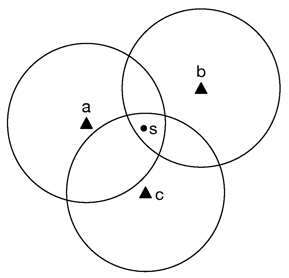
With the moving distance constraint, sensors can reach only some subareas. We construct a bipartite graph
. Each vertex
denotes a sensor in
. Each vertex
denotes a subarea covering a set of targets
. When the distance between sensor
i and subarea
is smaller than the constrained moving distance of sensor
i, that is,
, there is an edge between vertex
i and
j, where
is the minimum distance between sensor
i and subarea
j obtained in the pretreatment. The MTCLM problem is turning to be a matching problem except the weight is submodular. We formulate the MTCLM problem by an integer linear program (ILP) as following:
where
denotes if target
covered or not.
denotes if sensor
is scheduled to subarea
,
. The first constraint is the feasibility constraint, the second is the coverage constraint.
4.2. Randomized Algorithm
The Greedy algorithm presented above can not guarantee algorithm’s performance. Thus, we present three approximation algorithms which can make sure that the deviation of approximate solutions from the optimal value would not exceed a certain range. In this subsection, we propose a randomized approximation algorithm to obtain the expected value of the solution relative to the optimal value.
In this algorithm, we first obtain the optimal solution, and {}, of the Linear Program Relaxation (LPR) of formulas ILP, by replacing the constraints (4), (5) with and . Then for each vertex , we choose edge with prob. . Without changing the approximation ratio, we shift the covered targets by avoiding to cover the same subset. We run the algorithm for several times until we obtain the acceptable approximation solution.
Theorem 2. Algorithm 2 is a randomized -approximation algorithm for the MTCLM problem.
Proof. In this algorithm, the prob. for sensor
covering target
is
and each sensor
sends to cover subsets independently. Therefore, the overall prob. of not covering target
t sums up to
. According to Arithmeticgeometric mean inequality and the coverage constraint of ILP, we can show that
where
m denotes the maximal degree of any vertex in
in graph
G. Again, it holds algebraically that
. It then follows that the prob. of covering target
t in the algorithm is
Remind that
is the optimal value of LPR, bigger than the optimal value of ILP. Let
denote the optimal value of ILP. Then the expected number of covered targets is
It holds that the randomized rounding algorithm gives a randomized -optimal solution.
Linear programs can be solved in polynomial time and so is Algorithm 2. The theorem is proved. □
In Algorithm 2, we use the recycle variable
to avoid the sensors covering the same subset that would improve results and reduce instability in experiments.
| Algorithm 2: MTCLM_RANDOM (G, ). |
- Input:
graph G, - Output:
X,. - 1:
; - 2:
; - 3:
computer the optimal solution to the LP ,; - 4:
for eachdo - 5:
set a positive constant. - 6:
while do - 7:
set with probability ; - 8:
if then - 9:
set ; - 10:
- 11:
break; - 12:
else - 13:
set - 14:
; - 15:
end if - 16:
end while - 17:
end for - 18:
returnX,;
|
The method of conditional expectation can be used to derandomize the solution, but the computing complexity depends on the maximal degree
n of any vertex
in graph
G, that is, the maximal number of subareas a sensor can reach. We show the derandomized algorithm as below: Let
denote the set of vertices
for sensor
i.
. In each iteration
k,
is fixed. Set
to let the current conditional expectation maximized, that is,
, where
denotes the value of the LPR. After
M iterations, we can obtain deterministic
-optimal solution. In this algorithm,
linear programs need to be solved. At the worst cast,
is the number of vertices in
. The number of subareas
was proved in Reference [
34]. Thus,
at the worst case. That would make the time complexity of the derandomized algorithm too high. Even though, there are still lots of situations in which
n is constant in practical. With the moving distance constraint, each sensor is only allowed to reach a constant subarea, that is the derandomized algorithm suitable for.
Theorem 3. Algorithm 3 is a deterministic -approximation algorithm when n is constant.
Proof. As the explanation above, we prove the theorem by induction.
When , with no is fixed, is the expectation of the total number of covered targets. is proved in Theorem 2, where is the optimal solution of the ILP.
In each iteration k, where is fixed. And . We choose , thus .
After M iterations, the number of covered targets is .
To sum up, there are M iterations, and in each iteration, we need to solve at most n linear programs. Thus the time complexity is , assuming the time complexity of a linear program is . When each sensor is only allowed to reach a constant subarea, that is, n is a constant, Algorithm 3 is linearly solvable. Now, we prove that Algorithm 3 is a deterministic -approximation algorithm. □
| Algorithm 3: MTCLM_DERANDOMIZED(G, ). |
- Input:
graph G, - Output:
X,. - 1:
; - 2:
; - 3:
computer the optimal solution to the LP: ,; - 4:
for eachdo - 5:
; - 6:
set , ; - 7:
; - 8:
end for - 9:
return;
|
4.3. Deterministic Algorithm
The randomized algorithm needs to run several times to reduce instability. The derandomized algorithm can obtain an approximation solution determinately but costs too much time complexity at most time. In this subsection, we propose a deterministic algorithm to obtain a nearly
approximation value with less time complexity, where
is the maximal number of subsets covering the same target. Let
and
denote the optimal solution of the LPR. We round up each of them to the closest fraction of the form
,
H is a large integer and
a is an integer between 0 and
H. Mathematically, let
and
is defined similarly. (The rounding would incur a quantization error which we analysis later). For the graph
, we duplicate each node
to
identical nodes covering the same set of targets and connect each duplicated node to the neighbor of
j. We call the new graph the auxiliary graph
. We then find an edge-colouring of
such that any pair of edge sharing the same vertex in
is coloured differently. We can prove that
H colours are sufficient. We can show by pigeon-hole principle that we can always find a colour that the vertices in
covered by the edges in the colour cover at least
targets, that is,
. To prove this by contradiction, assuming that this is not true. Then the
It is leading to contradiction with the constraint (3) of the ILP.
The above analysis immediately implies that selecting the edges covered by the best coloured induced a
-optimal solution. More applications of the method can be seen in Reference [
39].
Each increases by at most by the rounding, hence increases the objective function by at most . Taking quantization error into consideration, the approximation ratio is . The auxiliary graph has at most nodes, edges, to find a proper coloration by greedy will take time . If we set , the approximation ratio is and the time complexity is . Thus we get the Theorem 4.
Theorem 4. Algorithm 4 is a nearly approximation algorithm
| Algorithm 4: MTCLM_COLOUR (G, ). |
- Input:
graph G, - Output:
X,. - 1:
; - 2:
; - 3:
computer the optimal solution to the LP: ,; - 4:
; - 5:
; - 6:
build auxiliary graph ; - 7:
obtain a legal colouring of greedily; - 8:
fordo - 9:
calculate the number of targets covered by each colour k; - 10:
end for - 11:
obtain colour q with the maximum number of covered targets; - 12:
obtain the edges coloured by q in graph ; - 13:
fordo - 14:
if is the duplication nodes of j in graph G then - 15:
set ; - 16:
; - 17:
end if - 18:
end for - 19:
return;
|


