3.2. Virtual Reference Point Generation
Each WiFi FP is composed of an RSS vector
(
M is the total number of detected APs in the entire dataset) and a location vector
. Considering a 3D coordinate system,
x,
y, and
z stand for the coordinate along
x,
y, and
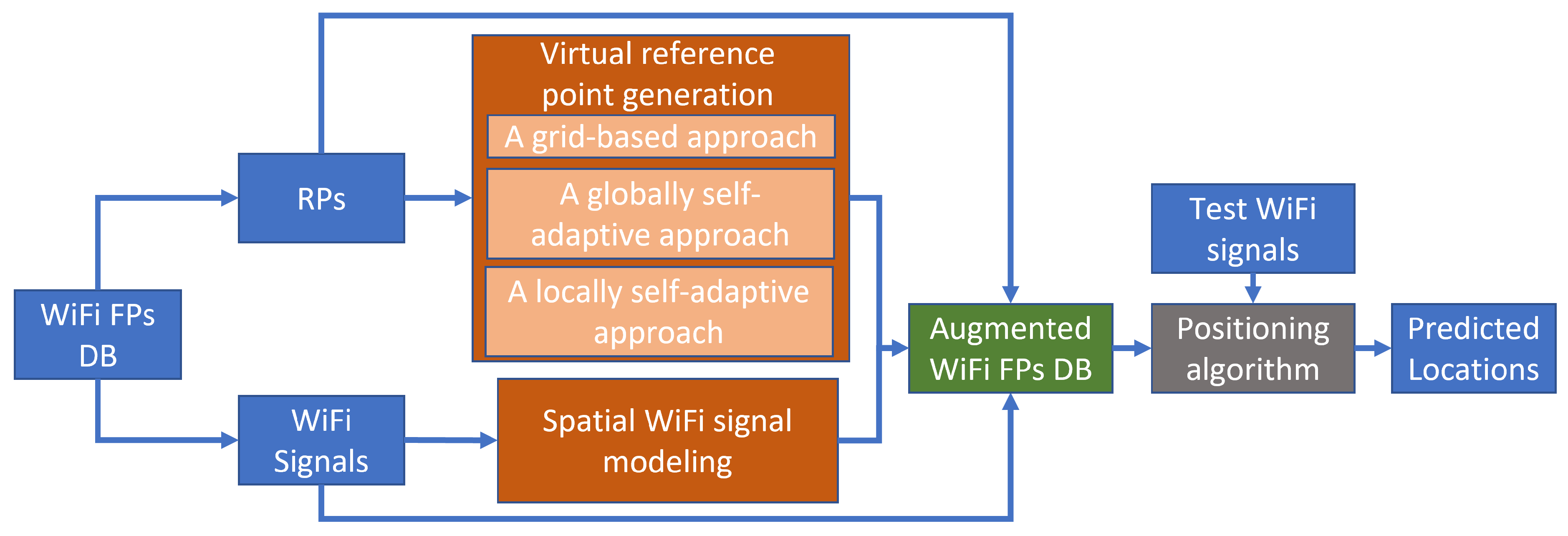
z-axis (in meters). To obtain more WiFi FPs for positioning, we first stipulate a strategy to determine the locations where they should be generated. In this study, based on the grid-based (GB) approach [
30] that was mentioned in the previous section, we propose two novel self-adaptive approaches: a globally self-adaptive (GS) approach and a locally self-adaptive (LS) approach.
3.2.1. A Grid-Based Approach
Before introducing the two proposed approaches, we first introduce the simple and well-adopted GB approach. For a certain floor at
h m, such an area can be simply described as a rectangle restrained by the maximum and minimum value of the coordinates of all the RPs along
x and
y-axes on the same floor, so that the four vertexes of such rectangle region are
,
,
and
. We define a virtual RP in the targeted region as
. The entire region is partitioned into multiple 1 × 1 m
2 grids along
x and
y axes. The coordinates of the virtual RPs are represented by the locations of the vertexes of each grid. So that:
hence, we can obtain
t virtual RPs, where
t can be calculated by:
One example of applying the GB approach to a specific floor is shown in
Figure 2.
3.2.2. A Globally Self-Adaptive Approach
Beyond the GB approach, we design a new GS approach to reduce the non-necessary virtual RPs outside the targeted region.
The GS approach first generates the virtual RPs the same as the GB approach. Then, Graham’s scan [
31] is used to detect the convex hull of the targeted region. Considering detecting the convex hull in a 2D environment on a floor, an initial RP with the lowest
y-coordinate is selected. Then, the rest of the RPs are sorted in increasing order of the angle calculated between them and the initial RP along the
z-axis. For the RPs with the same angle, only the farthest RP is kept (Euclidean distance is used to calculate the distance in this study). Then, we iterate the ordered RPs and calculate the angle formed by the three sequential RPs: previous RP, current RP, and next RP. The three RPs are kept if the angle is counterclockwise, or the current RP is dropped. Once the iteration finishes, the combination of the left RPs describes the convex hull of the targeted region, and only the virtual RPs that are inside the convex hull are kept.
To further remove the non-necessary virtual RPs, the virtual reference points are divided into many sub-areas by the mean-shift clustering algorithm. The mean-shift algorithm is a density-based unsupervised machine learning algorithm [
32]. It senses changes in data density and updates the centroid by computing the average shift vector over a given centroid at an arbitrary sample RP. Given a set of data
on a
d-dimensional space
, the mean shift vector of
can be expressed by:
where
is the kernel function and
h is the bandwidth (
in this study). The principle of mean shift is successively calculate the mean shift vector
and update the new
(
) until convergence.
The RPs eventually converge to the same centroid and are clustered in the same sub-areas. The virtual RPs in the sub-areas with no raw RPs are removed. One example of applying the GS approach to a specific floor is shown in
Figure 3.
3.2.3. A Locally Self-Adaptive Approach
Different from the previous two approaches, we also propose an LS approach that focuses on exploring the local distribution of the raw RPs and detecting where the virtual RPs should be generated. For a targeted region, the local approach first uses a mean-shift cluster algorithm to separate the region into several sub-areas from the training samples. Only sub-areas with three points and more are processed by Graham’s scan method to recognize their convex hulls. A similar scheme is adopted to generate virtual RPs in each sub-area. One example of applying the LS approach to a specific floor is shown in
Figure 4.
3.3. Spatial WiFi Signal Modeling
In this subsection, we present how we model the distributions of the spatial WiFi signal in a 3D environment to estimate the RSS values on the generated virtual RPs. For all RSS vectors
in
, and
in
, the mapping between the locations and the RSS vectors can be expressed by:
where
represents the independent and identically distributed Gaussian noise with zero mean and variance, which can be denoted by
.
To solve the mapping problem, we assume that all RSS vectors in the investigated indoor area obey a multivariate Gaussian process of multiple high-dimensional joint Gaussian distributions. Therefore, such a Gaussian process can be represented by the mean function
and covariance function
, as shown in the following equation:
where
denotes the expectation operator. Therefore, the covariance matrix
can be expressed by:
where
N denotes the total number of WiFi FPs (or the total number of RPs).
Through the grid-based RP algorithm mentioned in the previous subsection, we obtain
potential RPs
. This means that we have
new WiFi RSS vectors (FPs)
to be inferred. The RSS vectors
in the original dataset and RSS vectors
to be inferred should also follow a joint multivariate Gaussian distribution, which can be stated by the following equation:
The posterior distribution
can then be expressed as:
Hence, the posterior mean and covariance of the observed RSS vectors can be computed to obtain a model to predict the new RSS vectors on the unsurveyed potential RPs.
In addition, the covariance function
(also called kernel function) plays a vital role in a Gaussian process to denote the relation between the RSS vectors and the corresponding RPs. One popular kernel function is the squared exponential kernel, which assumes that the process of the system is very smooth [
33]. This is not suitable to describe the relationship among the high-dimensional RSS vectors in the large complex indoor scenario in our case. In [
28], a mixture of Matern and Rational Quadratic (RQ) kernels performs the best in capturing the variation of RSS values in comparison with other kernels. The Matern kernel is defined as:
where
denotes the smoothness of the function;
l is the length scale;
and
are the gamma function and the modified Bessel function [
33], respectively;
d is the Euclidean distance which can be calculated by:
The Rational Quadratic kernel can be described as:
where
stands for the shape parameter. Therefore, the mixed kernel in our case is designed as follows:
where
and
are the weighting parameters (initially set to 0.5). All the above-mentioned hyperparameters can be optimized by minimizing the negative logarithmic marginal likelihood.
After the MGPR model has been fine-tuned, it can forecast the RSS values for virtual RPs produced by the VRPG approaches, with the predicted RSS values presented in the same format as the training data. The predicted RSS values are then used to create new WiFi FPs, which are annotated with the location of the virtual RPs.


