
Long-Time Coherent Integration Method for Passive Bistatic Radar Using Frequency Hopping Signals


Abstract
:1. Introduction
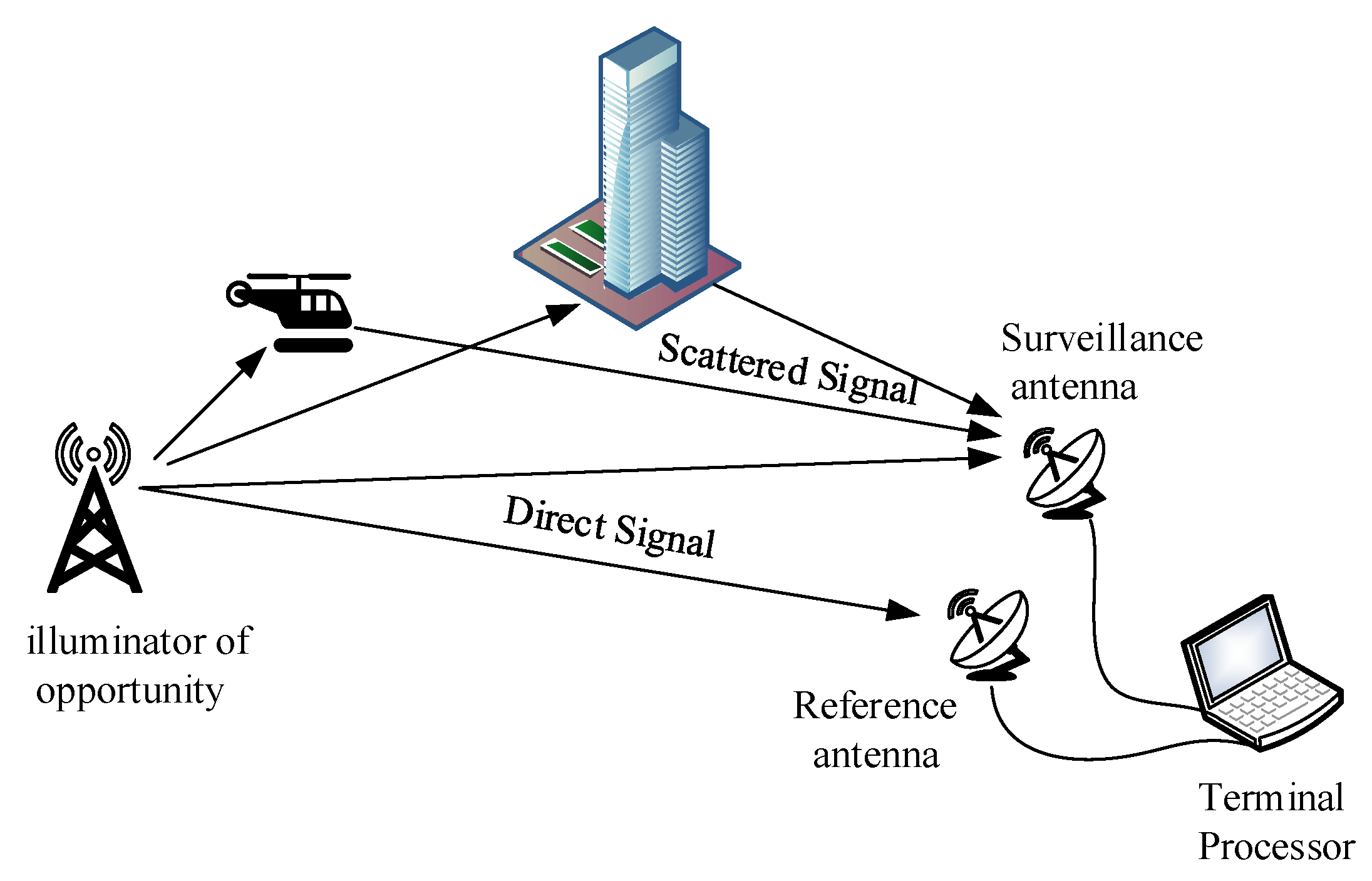
2. Signal Model
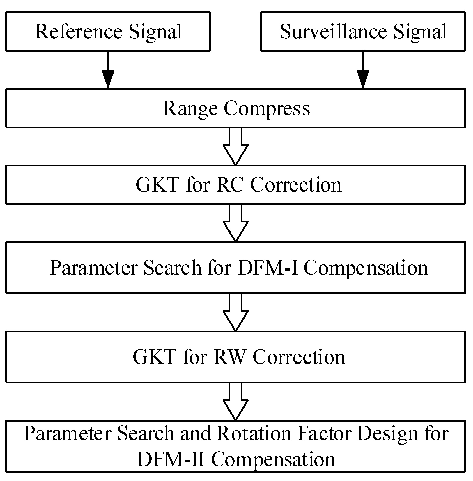
3. Proposed Method
3.1. Range Curve Correction
3.2. Doppler Frequency Migration-I Correction
3.3. Range Walk Correction
3.4. Doppler Frequency Migration-II Correction
| Algorithm 1 Summary: The main step of the proposed method |
| 1: Input: Original reference signal sref(t,tm) and surveillance signal ssur(t,tm), searching scope of target’s acceleration [amin, amax]. |
| 2: Fourier transform: Apply FT to sref(t,tm) and ssur(t,tm) with respect to fast time t to obtain Sref(f,tm) and Ssur(f,tm). |
| 3: Pulse compression: Apply pulse compression in frequency domain to obtain S(f,tm) by Equation (5). |
| 4: Range curve correction: Apply GKT to S(f,tm) and achieve S(f,τm) by Equation (7). |
| 5: DMF-I correction: Go through each a in [amin, amax]. |
| 6: For a = amin, …, amax |
| 7: Multiply the acceleration correction factor H(τm) and S(f,τm) to obtain Sa(f,τm) by Equation (9). |
| 8: Preserve the peak of Sa(f,τm). |
| 9: End |
| 10: Find the matched acceleration: Find the maximum peak value, the corresponding a is the estimated acceleration. |
| 11: Range walk correction: Apply GKT to Sa(f,τm) and achieve Sa(f,pm) by Equation (13). |
| 12: Inverse Fourier Transform: Convert Sa(f,pm) to pm-t domain form to obtain sa(t,pm) by Equation (14). |
| 13: Compensation factor calculation: Attribute the velocity compensation factor into the rotation factor of FT to obtain a new rotation factor Hw(pm,k) and design a new acceleration correction factor Ha(pm) according to the estimated acceleration a. |
| 14: DMF-II correction: Multiply sa(t,pm) and Ha(pm), then use Hw(pm,k) as a new rotation factor of FT to transform the multiplication result into the slow time frequency domain to obtain the coherent integration result Sa(t,Pm). |
4. Simulation Results
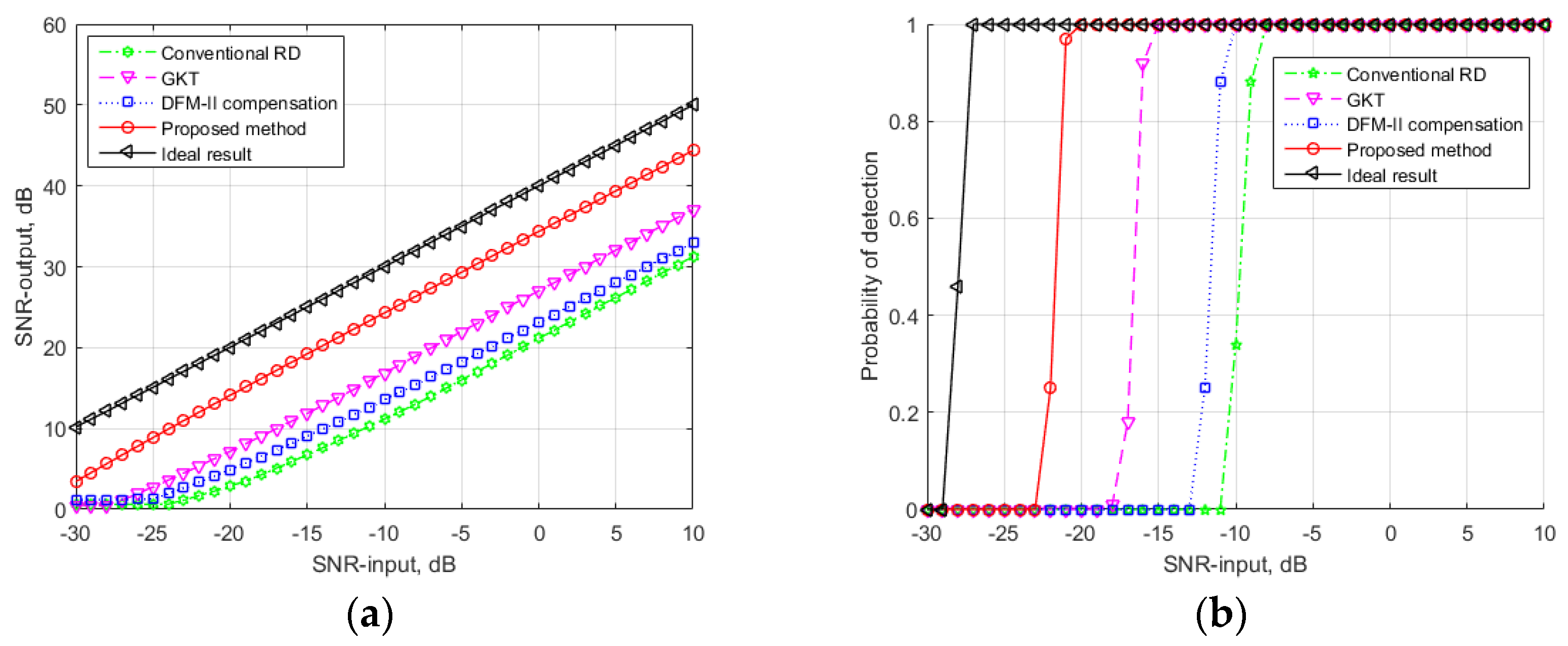
4.1. SNR Analysis
4.2. Computational Complexity
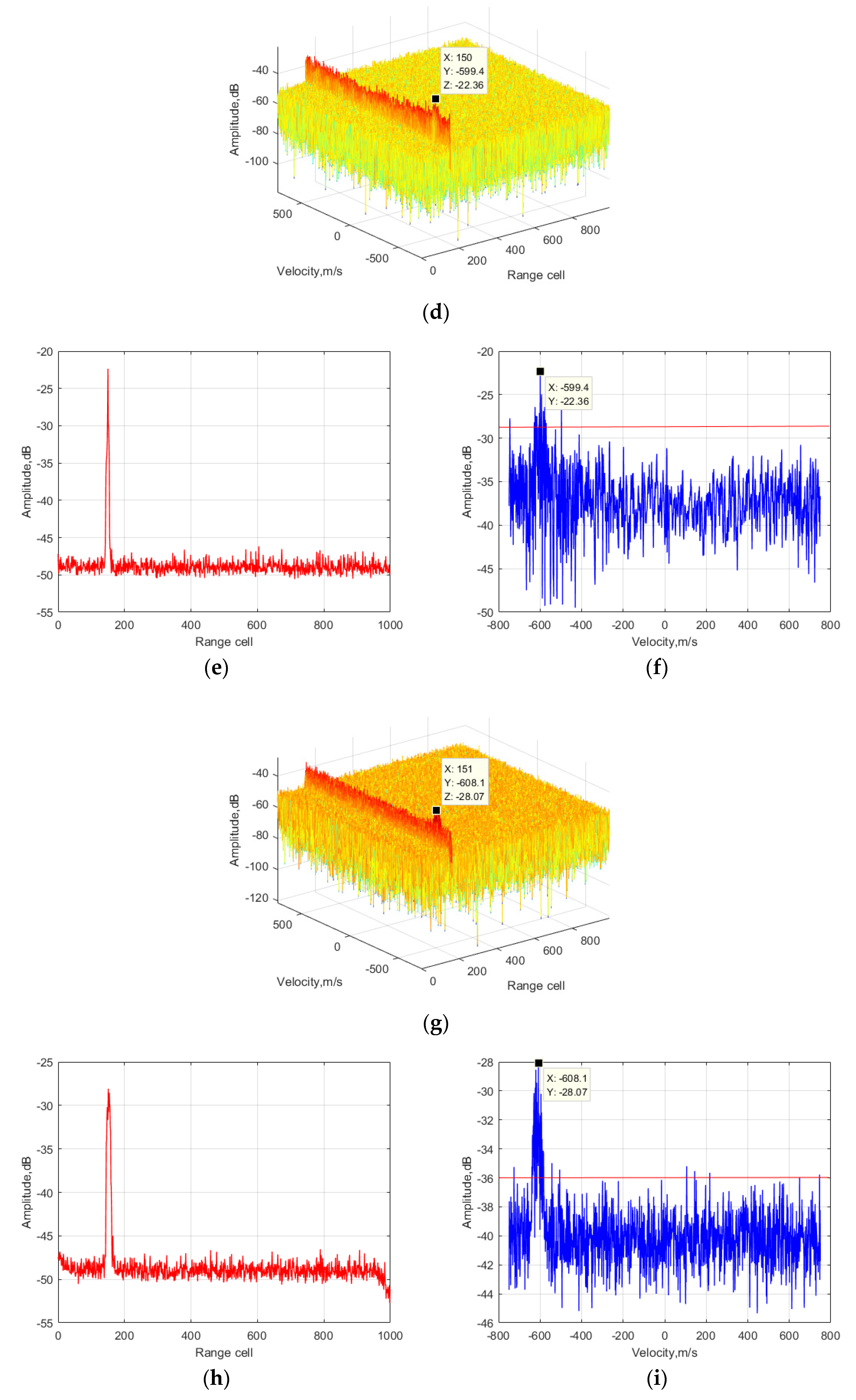
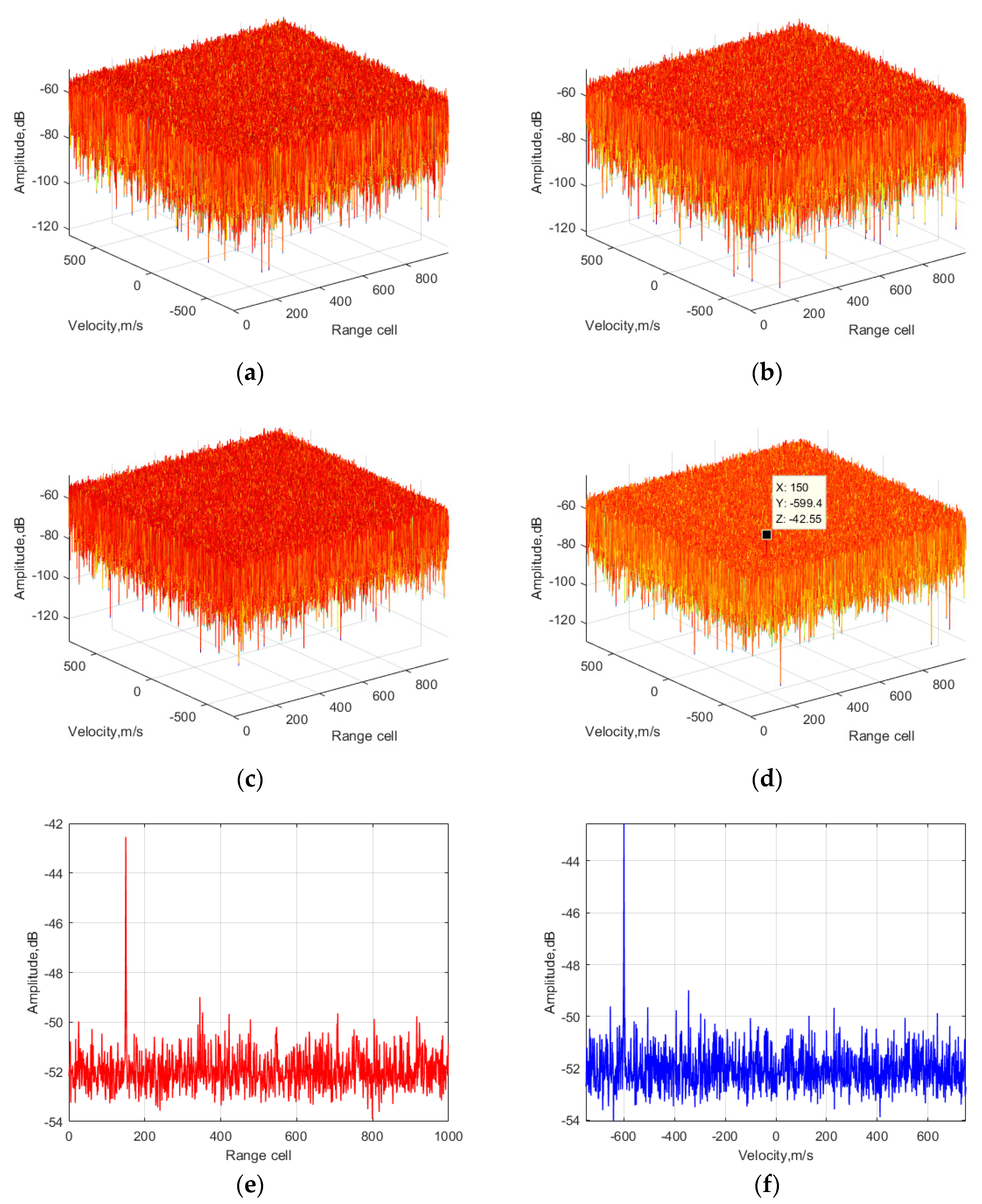
4.3. Integration Results
4.4. Performance Analysis
5. Conclusions
Author Contributions
Funding
Institutional Review Board Statement
Informed Consent Statement
Data Availability Statement
Acknowledgments
Conflicts of Interest
References
- Cui, K.; Wang, C.; Zhou, F.; Liu, C.; Gao, Y.; Feng, W. Fast Algorithm of Passive Bistatic Radar Detection Based on Batches Processing of Sparse Representation and Recovery. Remote Sens. 2024, 16, 2294. [Google Scholar] [CrossRef]
- Xie, D.; Yi, J.; Wan, X.; Jiang, H. Adaptive Model Mismatch Correction of Gridding Sparse Representation in Passive Radar. IEEE Sens. J. 2024, 24, 10594–10607. [Google Scholar] [CrossRef]
- Abratkiewicz, K.; Księżyk, A.; Płotka, M.; Samczyński, P.; Wszołek, J.; Zieliński, T.P. SSB-Based Signal Processing for Passive Radar Using a 5G Network. IEEE J. Sel. Top. Appl. Earth Observ. Remote Sens. 2023, 16, 3469–3484. [Google Scholar] [CrossRef]
- Malanowski, M.; Kulpa, K.; Kulpa, J.; Samczynski, P. Analysis of detection range of FM-based passive radar. IET Radar Sonar Navig. 2014, 8, 153–159. [Google Scholar] [CrossRef]
- Xie, D.; Yi, J.; Wan, X.; Jiang, H. Masking Effect Mitigation for FM-based Passive Radar via Nonlinear Sparse Recovery. IEEE Trans. Aerosp. Electron. Syst. 2023, 59, 8246–8262. [Google Scholar] [CrossRef]
- Park, D.H.; Park, G.H.; Park, J.H.; Bang, J.H.; Kim, D.; Kim, H.N. Interference Suppression for an FM-Radio-Based Passive Radar via Deep Convolutional Auto encoder. IEEE Trans. Aerosp. Electron. Syst. 2024, 60, 106–118. [Google Scholar] [CrossRef]
- Ummenhofer, M.; Lavau, L.C.; Cristallini, D.; O’Hagan, D. UAV Micro-Doppler Signature Analysis Using DVB-S Based Passive Radar. In Proceedings of the 2020 IEEE International Radar Conference, Washington, DC, USA, 28–30 April 2020; pp. 1007–1012. [Google Scholar] [CrossRef]
- Del-Rey-Maestre, N.; Jarabo-Amores, M.P.; Mata-Moya, D.; Almódovar-Hernández, A.; Rosado-Sanz, J. Planar Array and spatial filtering techniques for improving DVB-S based passive radar coverage. In Proceedings of the 2022 19th European Radar Conference, Milan, Italy, 28–30 September 2022; pp. 1–4. [Google Scholar] [CrossRef]
- Sjögren, T.; Tryblom, A.; Ragnarsson, R.; Jonsson, O. Impact of Transmitter Elevation Pattern on Multi-frequency DVB-T Passive Radar Detection of Airborne Targets. In Proceedings of the 2023 IEEE International Radar Conference, Sydney, Australia, 6–10 November 2023; pp. 1–6. [Google Scholar] [CrossRef]
- Rodriguez, J.T.; Blasone, G.P.; Colone, F.; Lombardo, P. Exploiting the Properties of Reciprocal Filter in Low-Complexity OFDM Radar Signal Processing Architectures. IEEE Trans. Aerosp. Electron. Syst. 2023, 59, 6907–6922. [Google Scholar] [CrossRef]
- Edrich, M.; Schroeder, A.; Meyer, F. Design and performance evaluation of a mature FM/DAB /DVB-T multi-illuminator passive radar system. IET Radar Sonar Navig. 2014, 8, 114–122. [Google Scholar] [CrossRef]
- Hu, S.; Yi, J.; Wan, X.; Cheng, F.; Hu, Y.; Hao, C. Illuminator of Opportunity Localization for Digital Broadcast-Based Passive Radar in Moving Platforms. IEEE Trans. Aerosp. Electron. Syst. 2023, 59, 3539–3549. [Google Scholar] [CrossRef]
- Narayanan, R.M.; Handel, C.F. Vehicle Length Estimation Using an LTE Transmitter Combined with a Software-Defined Receiver. IEEE Sens. Lett. 2021, 5, 3500704. [Google Scholar] [CrossRef]
- Dan, Y.; Xu, K.; Yi, J.; Wan, X. Reference Signal Fractionation for LTE-Based Passive Radar Facing MIMO and OFDMA Challenges. IEEE Sens. J. 2024, 24, 12904–12916. [Google Scholar] [CrossRef]
- Huang, C.; Li, Z.; An, H.; Sun, Z.; Wu, J.; Yang, J. Maritime Moving Target Detection Using Multiframe Recursion Association in GNSS-Based Passive Radar. IEEE Sens. J. 2024, 24, 6380–6391. [Google Scholar] [CrossRef]
- Zhang, C.; Shi, S.; Yan, S.; Gong, J. Moving Target Detection and Parameter Estimation Using BeiDou GEO Satellites-Based Passive Radar with Short-Time Integration. IEEE J. Sel. Top. Appl. Earth Observ. Remote Sens. 2023, 16, 3959–3972. [Google Scholar] [CrossRef]
- Daniel, L.; Hristov, S.; Lyu, X.; Stove, A.G.; Cherniakov, M.; Gashinova, M. Design and Validation of a Passive Radar Concept for Ship Detection Using Communication Satellite Signals. IEEE Trans. Aerosp. Electron. Syst. 2017, 53, 3115–3134. [Google Scholar] [CrossRef]
- Blázquez-García, R.; Cristallini, D.; Ummenhofer, M.; Seidel, V.; Heckenbach, J.; O’Hagan, D. Experimental comparison of Starlink and OneWeb signals for passive radar. In Proceedings of the 2023 IEEE Radar Conference, San Antonio, TX, USA, 1–5 May 2023; pp. 1–6. [Google Scholar] [CrossRef]
- Zhu, S.; Liao, G.; Yang, D.; Tao, H. A New Method for Radar High-Speed Maneuvering Weak Target Detection and Imaging. IEEE Geosci. Remote Sens. Lett. 2014, 11, 1175–1179. [Google Scholar] [CrossRef]
- Winters, D.W. Target Motion and High Range Resolution Profile Generation. IEEE Trans. Aerosp. Electron. Syst. 2012, 48, 2140–2153. [Google Scholar] [CrossRef]
- Li, Z.; Huang, C.; Sun, Z.; An, H.; Wu, J.; Yang, J. BeiDou-Based Passive Multistatic Radar Maritime Moving Target Detection Technique via Space–Time Hybrid Integration Processing. IEEE Trans. Geosci. Remote Sens. 2022, 60, 5802313. [Google Scholar] [CrossRef]
- Perry, R.P.; DiPietro, R.C.; Fante, R.L. SAR imaging of moving targets. IEEE Trans. Aerosp. Electron. Syst. 1999, 35, 188–200. [Google Scholar] [CrossRef]
- Xu, J.; Yu, J.; Peng, Y.N.; Xia, X.G. Radon-Fourier Transform for Radar Target Detection, I: Generalized Doppler Filter Bank. IEEE Trans. Aerosp. Electron. Syst. 2011, 47, 1186–1202. [Google Scholar] [CrossRef]
- Huang, Z.; Wang, J.; Sui, J.; Zuo, L.; Cheng, Z. Multiframe Integration Method via Short-Time Radon Lv’s Distribution for Passive Bistatic Radar. IEEE Sens. J. 2024, 24, 16529–16539. [Google Scholar] [CrossRef]
- Zuo, L.; Wang, J.; Wang, J.; Chen, G. UAV detection via long-time coherent integration for passive bistatic radar. Digit. Signal Process. 2021, 112, 102997. [Google Scholar] [CrossRef]
- Zuo, L.; Han, J.; Yan, Y.; Yeo, T.-S.; Lu, B.; Wang, Y.; Xue, S.; Wang, M.; Wang, Z.; Shi, H.; et al. Multi-Frequency Coherent Integration Target Detection Algorithm for Passive Bistatic Radar. In IEEE Transactions on Aerospace and Electronic Systems; IEEE: Toulouse, France, 2024. [Google Scholar] [CrossRef]
- Kirkland, D. Imaging moving targets using the second-order keystone transform. IET Radar Sonar Navig. 2011, 5, 902–910. [Google Scholar] [CrossRef]
- Li, X.; Cui, G.; Yi, W.; Kong, L.; Yang, J. Range migration correction for maneuvering target based on generalized keystone transform. In Proceedings of the IEEE Radar Conference, Arlington, VA, USA, 10–15 May 2015. [Google Scholar] [CrossRef]
- Li, X.; Cui, G.; Yi, W.; Kong, L. Coherent Integration for Maneuvering Target Detection Based on Radon-Lv’s Distribution. IEEE Signal Process. Lett. 2015, 22, 1467–1471. [Google Scholar] [CrossRef]
- Chen, X.; Guan, J.; Liu, N.; He, Y. Maneuvering Target Detection via Radon-Fractional Fourier Transform-Based Long-Time Coherent Integration. IEEE Trans. Signal Process. 2014, 62, 939–953. [Google Scholar] [CrossRef]
- Tao, R.; Zhang, N.; Wang, N.Y. Analysing and compensating the effects of range and Doppler frequency migrations in linear frequency modulation pulse compression radar. IET Radar Sonar Navig. 2009, 5, 12–22. [Google Scholar] [CrossRef]
- Chang, S.; Deng, Y.; Zhang, Y.; Zhao, Q.; Wang, R.; Zhang, K. An Advanced Scheme for Range Ambiguity Suppression of Spaceborne SAR Based on Blind Source Separation. IEEE Trans. Geosci. Remote Sens. 2022, 60, 5230112. [Google Scholar] [CrossRef]
- Filip-Dhaubhadel, A.; Shutin, D. Long Coherent Integration in Passive Radar Systems Using Super-Resolution Sparse Bayesian Learning. IEEE Trans. Aerosp. Electron. Syst. 2021, 57, 554–572. [Google Scholar] [CrossRef]
- Ma, B.; Zhang, S.; Jia, W.; Wang, W. Fast Implementation of Generalized Radon-Fourier Transform. IEEE Trans. Aerosp. Electron. Syst. 2021, 57, 3758–3767. [Google Scholar] [CrossRef]
- Huang, P.; Liao, G.; Yang, Z.; Xia, X.G.; Ma, J.T.; Ma, J. Long-Time Coherent Integration for Weak Maneuvering Target Detection and High-Order Motion Parameter Estimation based on Keystone Transform. IEEE Trans. Signal Process. 2016, 64, 4013–4026. [Google Scholar] [CrossRef]
- Huang, P.; Liao, G.; Yang, Z.; Ma, J. An approach for refocusing of ground fast-moving target and high-order motion parameter estimation using radon-high-order time-chirp rate transform. Digit. Signal Process. 2016, 48, 333–348. [Google Scholar] [CrossRef]
- Zeng, C.; Li, D.; Luo, X.; Song, D.; Liu, H.; Su, J. Ground Maneuvering Targets Imaging for Synthetic Aperture Radar Based on Second-Order Keystone Transform and High-Order Motion Parameter Estimation. IEEE J. Sel. Top. Appl. Earth Observ. Remote Sens. 2019, 12, 11. [Google Scholar] [CrossRef]
- Gu, M.X.; Lee, M.C.; Liu, Y.S.; Lee, T.S. Design and Analysis of Frequency Hopping-Aided FMCW-Based Integrated Radar and Communication Systems. IEEE Trans. Commun. 2022, 70, 8416–8432. [Google Scholar] [CrossRef]
- Chen, G.; Wang, J.; Zuo, L.; Zhao, D. Long-Time Coherent Integration for Frequency Hopping Pulse Signal via Phase Compensation. IEEE Access 2020, 8, 30458–30466. [Google Scholar] [CrossRef]
- Chen, G.; Wang, J.; Zuo, L.; Wen, Y. Two-stage clutter and interference cancellation method in passive bistatic radar. IET Signal Process. 2020, 14, 342–351. [Google Scholar] [CrossRef]


| Parameters | Values |
|---|---|
| Center frequency | 1 GHz |
| Frequency hopping bandwidth | 100 MHz |
| Signal bandwidth | 5 MHz |
| Sampling frequency | 5 MHz |
| Observation time | 0.12 s |
| Pulse duration | 0.5 µs |
| Pulse repetition time | 1 µs |
| Pulse number | 1200 |
| Target’s initial range cell | 150 |
| Target’s initial velocity | −600 m/s |
| Target’s acceleration | −200 m/s2 |
| Target’s SNR | −10 dB |
| Step | Computational Complexities |
|---|---|
| FFT operation on reference and surveillance signals | 2MNlog2N |
| Pulse compression operation in frequency domain | MN |
| CZT in RC and RW correction | 2N(L + 2M + 1.5Llog2L + 0.5Mlog2M) |
| Acceleration estimation in DFM-I and DFM-II | 2Mlog2M |
| FFT operation on correction result | 2MNlog2N |
| Velocity compensation in DFM-II | 2MN2 |
Disclaimer/Publisher’s Note: The statements, opinions and data contained in all publications are solely those of the individual author(s) and contributor(s) and not of MDPI and/or the editor(s). MDPI and/or the editor(s) disclaim responsibility for any injury to people or property resulting from any ideas, methods, instructions or products referred to in the content. |
© 2024 by the authors. Licensee MDPI, Basel, Switzerland. This article is an open access article distributed under the terms and conditions of the Creative Commons Attribution (CC BY) license (https://creativecommons.org/licenses/by/4.0/).
Share and Cite
Chen, G.; Biao, X.; Jin, Y.; Xu, C.; Ping, Y.; Wang, S. Long-Time Coherent Integration Method for Passive Bistatic Radar Using Frequency Hopping Signals. Sensors 2024, 24, 6236. https://doi.org/10.3390/s24196236
Chen G, Biao X, Jin Y, Xu C, Ping Y, Wang S. Long-Time Coherent Integration Method for Passive Bistatic Radar Using Frequency Hopping Signals. Sensors. 2024; 24(19):6236. https://doi.org/10.3390/s24196236
Chicago/Turabian StyleChen, Gang, Xiaowei Biao, Yi Jin, Changzhi Xu, Yifan Ping, and Sujun Wang. 2024. "Long-Time Coherent Integration Method for Passive Bistatic Radar Using Frequency Hopping Signals" Sensors 24, no. 19: 6236. https://doi.org/10.3390/s24196236