1. Introduction
Wind power has become increasingly important as an efficient, renewable energy source in recent decades. The number of wind turbines is increasing from year to year [
1]. With more than 17,000 blades now in use worldwide, it is estimated that 3800 are certainly damaged [
2]. The common types of damage that can destroy a rotor blade include delamination, debonding, and cracks [
3]. This damage usually starts small and grows until the blade collapses. Only close monitoring can detect damage during growth and prevent further damage and costs. The currently applied comprehensive monitoring is carried out by trained industrial climbers. With costs of several thousand dollars per inspection on land and several tens of thousands of dollars offshore, these inspection significantly reduce the profitability of the plants [
4]. These circumstances motivate the development of automated, permanent monitoring systems for wind turbines: so-called structural health monitoring systems. The most common and most widely researched systems are based on voltage measurements, acoustic emission, vibration, and ultrasound [
5]. Radar-based monitoring approaches offer a number of important advantages in structural monitoring, such as non-contact measurement and the monitoring of large areas. For this reason, the use of radar devices in the monitoring of wind turbines is an increasingly important aspect of research. The approaches to date monitor the rotor blades with sensors from the tower or from the ground, as presented by Nikoubin et al. [
6], Zhao and Hong [
7], and Mälzer et al. [
8].
A new approach integrates the radar sensors directly into the rotor blades with the best possible distribution, determined by simulation. A total of 40 low-cost FMCW radar sensors monitor the entire rotor blade with redundancy and the option for triangulation. Each sensor can monitor the entire environment but only requires a limited field of view. The disadvantages of radar sensors listed by Sun et al. [
9] in their overview of monitoring technologies for wind turbines, such as high transmission power and increased power consumption, are thereby relativized. The disadvantage remains in that radar sensors are susceptible to operational and environmental changes. Structural changes, such as damage, change the measured signal. These changes enable an automated system to detect damage. If temperature influences change the signal to a similar extent, damage can go unnoticed or the system can be falsely triggered even though there is no damage.
Temperature influences the measured radar signals through several physical effects. A first, very obvious effect is the temperature-dependent change in the physical properties of the observed environment. The permittivity of the glass fiber reinforced plastics (GFRP) and core materials of the rotor blade, which is primarily important for radar measurements, changes [
10,
11]. This directly influences the reflection, transmission, and dispersion behavior of electromagnetic waves. Secondly, the temperature has an influence on the electronics of the sensor itself [
12,
13]. Due to changing conductivities, temperature-dependent changes also occur in the analog-to-digital converter (ADC) and digital-to-analog converter (DAC).
The temperature influence of FMCW radar sensors has also been shown in a variety of works. For example, climate chamber experiments show the influence of temperature and humidity on radar measurements [
14]. In the calibration of cloud radars according to Toledo et al. [
15], temperature plays a decisive role. These observations strongly imply that an SHM system, which by its very nature should have a high level of accuracy, take any influences into account, and compensate for them if necessary. However, the influence of temperature and other environmental influences has not yet been addressed in radar-based monitoring approaches for wind turbines.
For this reason, this work uses the data from a large-scale experiment to analyze this temperature influence. In a full-scale fatigue test, several damages were caused in a 31 m long rotor blade due to overloading. In addition, temperature fluctuations of several degrees were recorded by each radar sensor during the experiment. The radar data from an intact and a damaged rotor blade at temperature change offer an opportunity to compare the effects of temperature and damage and to evaluate the influence on SHM systems. In order to minimize temperature influences and maximize the sensitivity of radar-based SHM systems, several temperature compensation methods are then considered. A first approach is the seasonal trend decomposition, which determines a trend on the periodic radar signals and can thus eliminate it. Due to the effect of the different temperature influences on the signals, this method proved to be only a slight improvement. A further development significantly improves the compensation of temperature influences. To classify the new method, the results for some selected sensors are compared with the results of the optimal baseline selection (OBS), introduced in ultrasound SHM systems [
16], and discussed.
2. Materials and Methods
2.1. Data Acquisition
The data were recorded during a full-scale fatigue test. For this purpose, a 31 m long rotor blade in an experimental hall was subjected to a load test according to IEC 61400-23:2014-04 [
17]. In incremental steps, the load was increased to such an extent that damage occurred and finally a crack destroyed the blade. A drawing of the blade with some important sensors can be seen in
Figure 1. During the experiment, visual inspections were carried out by trained workers and a large number of small damages to the GRP material were documented. In particular, micro-damage in the form of fiber breaks, as shown in
Figure 2, occurred across the entire surface. However, the frequency and severity decreases towards the tip, as the sheet was less severely deformed there. This crack can also be seen in
Figure 2 on the right. The blade was loaded edge-wise with a piston. Wooden load frames were mounted to provide an optimal load distribution and are illustrated in
Figure 1. These load frames have been removed from time to time for vibration analyses and then reinstalled in approximately the same position. Therefore, exact positioning could not be guaranteed and minor structural changes can be expected near any of the load frames.
In order to eliminate any possible influences on the radar signals caused by deformation of the blade, only data from test pauses when the blade was stationary are used in this work. During these test pauses, however, the blade was exposed to environmental influences inside the experimental hall.
A total of 40 radar sensors were placed in the rotor blade. Of these 40 radar sensors, 10 sensors are embedded in the rotor blade material and will not be considered further here, as they behave very individually and completely differently to the glued-on sensors. The embedding in GFRP structures of different thicknesses, depending on the position in the blade, and in particular the unique positioning of glass fiber fabric directly in front of the sensors, makes a holistic analysis impossible. A total of 8 sensors (and a total of 6 glued-on sensors) were damaged during production and were therefore unusable. The low-cost radar sensors used consisted of a BGT60TR13C FMCW 60 GHz radar from Infineon Technologies (Neubiberg, Germany) with a bandwidth of 5.5 GHz, sub-GHz communication, an LIS3DH acceleration sensor including a temperature sensor, and a microcontroller for control.
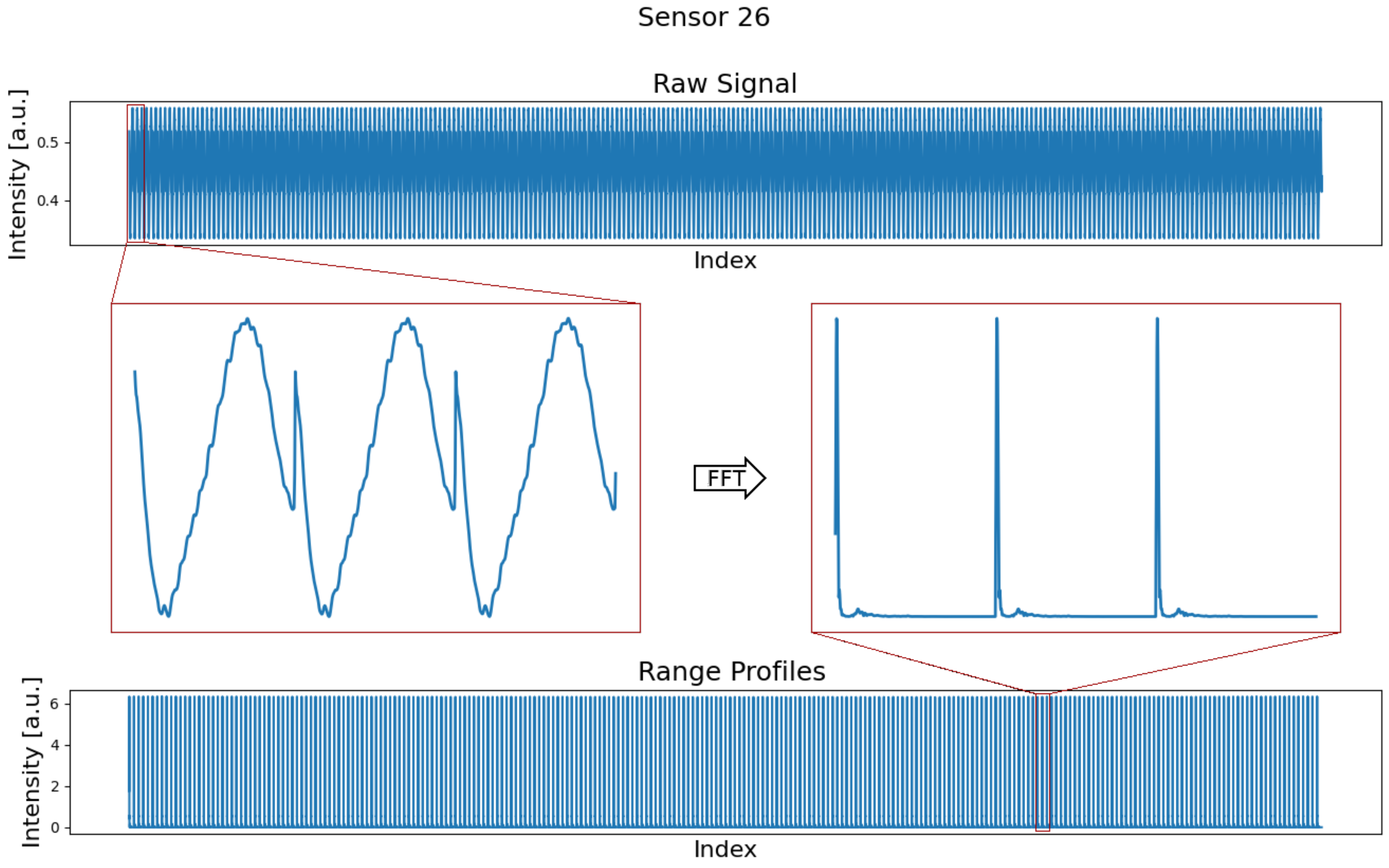
The BGT60TRC has 1 transmitting and 3 receiving antennas integrated in a package. The FMCW radar has a spatial resolution of around 2.5 cm and a range of 3.5 m. As is usual with FMCW radar sensors, the transmitted signal is mixed with the emitted signal. By calculating an FFT on the mixed signal, distance-dependent amplitudes, so-called range profiles
s, can then be generated. The raw measured signal and the calculated range profiles are shown in
Figure 3. The sensors are housed in a 3D-printed casing. In order to eliminate any reflections from the housing and near-field artifacts, gating is applied to the range profiles and only amplitudes from 0.2 m are considered.
While the data are transmitted via wireless communication, the sensors are supplied with power via cables. These cables are fixed every few centimeters, but it is conceivable that they can move slightly due to the load on the blade. A more detailed description of the experiment can be found in [
18].
2.2. Seasonal Trend Decomposition
The seasonal trend decomposition works for measured data
, that is, either the sum
of a seasonal part
, a trend
and a residual
, or the quotient
of these terms [
19]. This means that the additive approach assumes that an additive trend lies above the periodic data and the multiplicative approach assumes that a trend scales each data point of the periodic signal. In our problem, the periodic data correspond to the range profiles with 512 data points.
In either case, the trend is then estimated using a moving average
with the order
, where
k corresponds to the periodicity and is therefore 512. The moving average is based on the common implementation for seasonal trend decomposition with a window in the form
What is special here is that the points with the same index in the previous and subsequent range profile are only weighted with 0.5.
On the basis of the various influences described (influences on the electronics, temperature-dependent change in permittivity and thus change in reflection and dispersion) and their complex superposition, it is not immediately obvious whether the temperature trend is additive or multiplicative in the case of radar signals. Looking at the phase term [
20]
which can be used to calculate the dispersion and signal strength, it can be assumed that temperature changes are multiplicative rather than additive.
A comparative application of the additive and multiplicative method quickly shows that a multiplicative trend reduces the temperature influence while the additive approach does not provide any useful results. From this observation, it can be concluded that a multiplicative approach must be chosen for temperature trends in the case of radar signals. Accordingly, we obtain the adjusted range profiles based on separation of the seasonal part with
where the residual containing, i.e., noise cannot be separated.
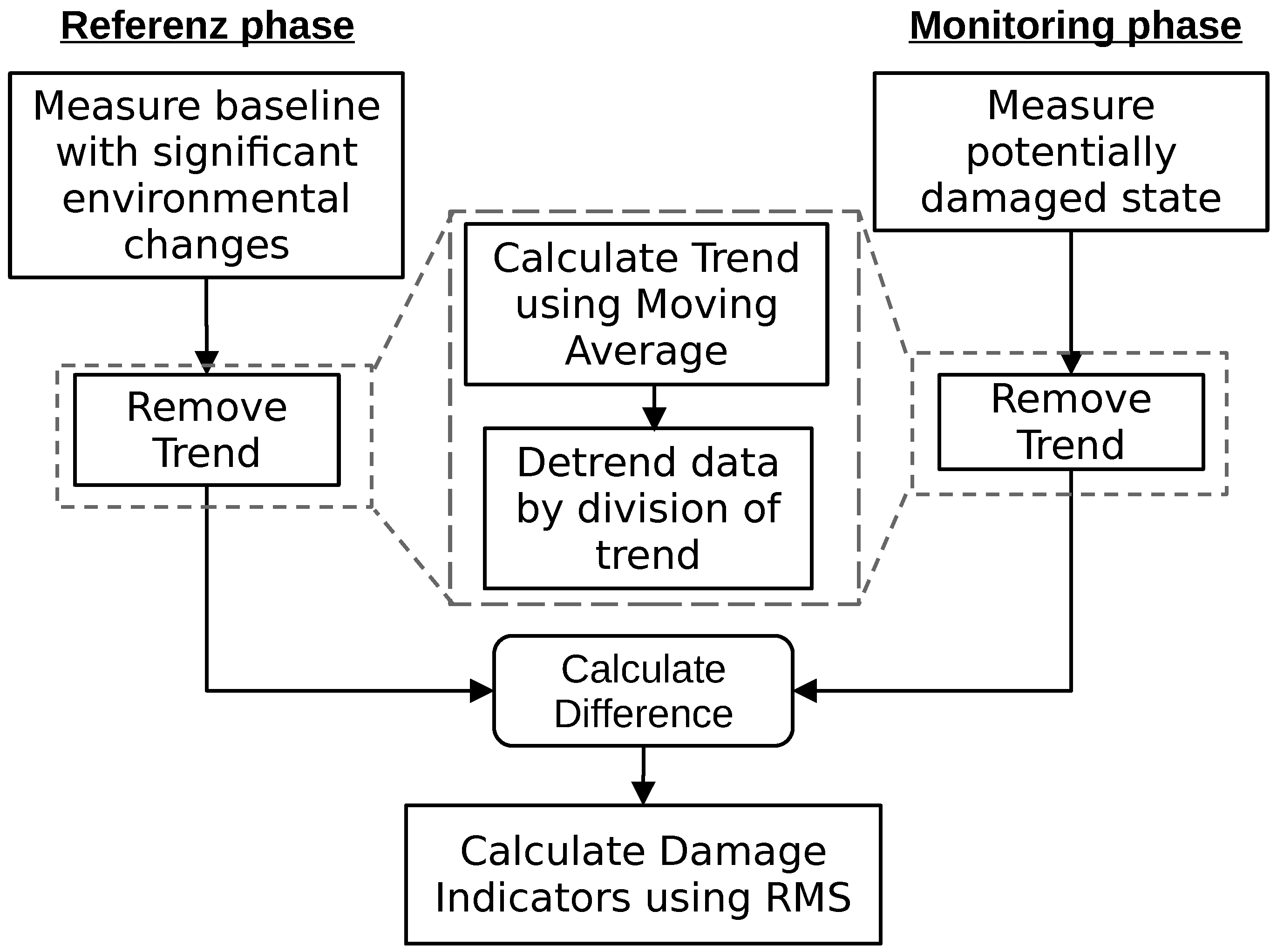
The procedure with which a structural health monitoring system with the described trend compensation would work is described in
Figure 4.
2.3. Bin-Specific Trend Compensation
With bin-specific trend compensation (BSTC), a separate trend is determined for each range bin of a series of range profiles. This differs from seasonal trend decomposition, where all points of a range profile share the same trend. This is implemented using slices with a periodicity interval
k on the original data set. For this purpose, all points except the indices −(
k + 1), 0 and
k + 1 are removed from the moving average filter (
4).
k here again corresponds to the length of the given range profiles of 512. The filter becomes
The formula for the trend adapted to a single bin
t is
with the periodicity
k. The formula forms the mean value for the range bin
i under consideration with the same range bin
of the previous measurement and the range bin
of the subsequent measurement.
Here, it is no longer possible to simply divide by the trend, as otherwise the ratio between the bins of a range profile would vanish. After dividing by the determined trend, the mean value of each bin would be equal to 1. Therefore, the trend relative to the respective mean value
of the bin is eliminated. This must be carried out for each bin
b =
. The temperature-independent signal is derived from
A decisive effect that the seasonal trend decomposition has on the seasonal signal
is that the mean value of the seasonal component
after adjustment is always the same and independent of the size of
. For this reason, each range profile is also divided by the mean value in bin-specific trend compensation after adjustment of the trends.
While the adjustment of the trend works differently, the workflow is the same as in
Figure 4.
2.4. Optimal Baseline Selection
For the optimal baseline selection, a number of baselines with equidistant temperature steps is created. A simple way to obtain these baselines is to extract them from a continuous measurement by averaging the measurements within a sized bin. For a measurement at temperature T, the baseline is used for evaluation, where is minimal.
The procedure used by a structural health monitoring system with optimal baseline selection is described in
Figure 5.
2.5. Thresholds
To estimate structural damage based on measured data, a threshold value is usually used for adjustment. If the measurement data exceed the threshold value, the monitoring system assumes a material failure and reacts. The determination of a suitable threshold value is not trivial. A common approach is to calculate the 99th percentile from a set of reference data as the threshold. However, with the 99th percentile, measurements were already above the threshold during the reference period. Outliers in the measurement data may again exceed the threshold. Therefore, one usually requires that several measurements in a row exceed the threshold. As we will see later, the maximum values of our radar measurement are adjacent to each other due to temperature dependence, so this mechanism alone may not be sufficient to prevent false alarms. To ensure that no measurement in the reference condition would trigger an alarm, we add the standard deviation to the 99th percentile and require that this threshold is exceeded five times. In this definition of the threshold, the standard deviation has the advantage that the threshold is correspondingly higher in the case of strongly fluctuating values. The threshold value based on a set of damage indicators
is thus calculated with
From the radar data as range profiles, which consist of a set of distance-dependent amplitudes, single values must be made for the comparison with a threshold value. For this purpose, the root mean square (RMS)
of the differences of signal
s and baseline
b is calculated as damage indicator
.
4. Discussion
The data from the fatigue test showed that temperature influences the radar signals significantly. This can even lead to temperature effects being greater than the signal change due to structural changes and damage. In addition, the temperature here only changed by around 6 °C, whereas temperatures at a wind turbine in the field can change by more than 10 °C over the course of the day and by more than 30 °C between winter and summer. Temperature compensation increases the sensitivity of an SHM system and is therefore absolutely essential. For sensors close to the large crack, such as sensor 1 and sensor 20, compensation is not absolutely necessary to detect damage. However, in the case of sensor 26, which is shown here in great detail, the many documented small damages only become visible when the temperature of the crack is higher than the temperature of the crack.
A detailed analysis of the range profiles in the
Figure 7 and
Figure 11 shows that each range bin has a very individual temperature dependence. Motivated by this, the adaptation of the seasonal trend decomposition results in a new method that determines a corresponding trend for each bin. This so-called bin-specific trend compensation (BSTC) shows much better results than looking at the range profiles as seasonal data. The reason for this is that the range profiles do not have a global trend, but each range bin has its own trend. The reason for this in turn lies in the various temperature-dependent effects, which combine to varying degrees in the bins. A bin that does not contain any significant reflections is only affected by influences on the electronics. A bin that contains the reflections of several objects or surfaces is affected by a complex combination of influences on the electronics, the reflections and transmissions, and multiscattering.
The BSTC also shows very good results in comparison to optimal baseline selection. The realization that each bin has its own trend, which is determined by the environment and the echoes, explains why also OBS works so well for radar signals. The baselines at equidistant temperatures provide a discrete function for each bin. This allows to compensate the temperature-dependent behavior well, as long as there is a baseline close to the current temperature.
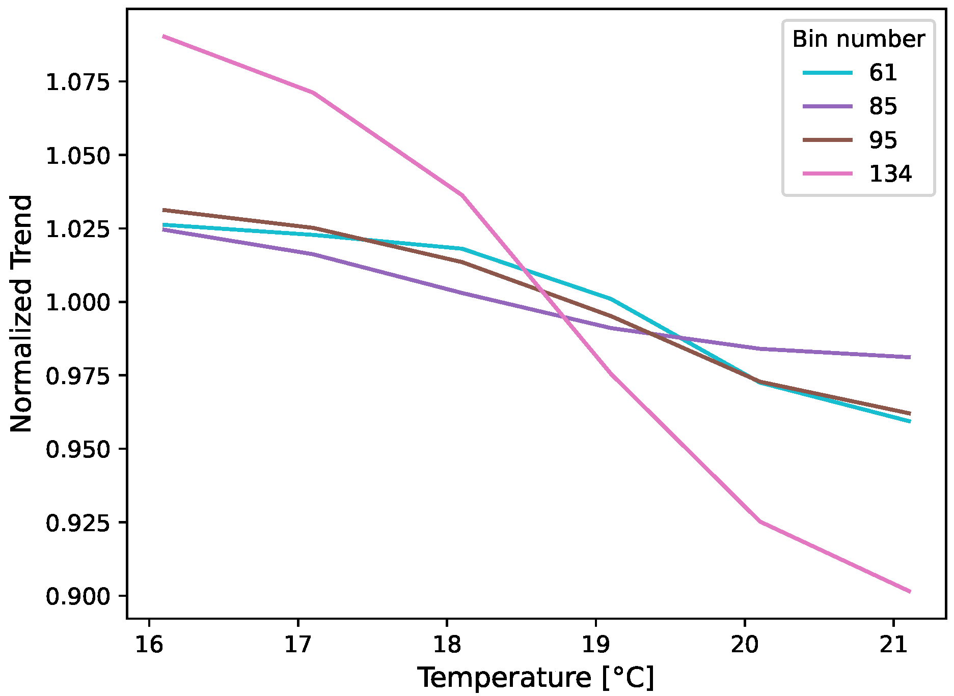
By dividing the trend, the level of data is adjusted in the seasonal trend decomposition. This is no longer the case with bin-specific analysis, where the bins are adjusted relative to their mean value, as otherwise the relationship between the bins and thus the amplitudes would be lost. As long as the states or measurements to be compared take place in comparable temperature ranges or more precisely, as long as the mean values of measurement series are similar, the trend compensation works excellently. The BSTC was divided by the mean value in order to equalize the absolute values at different ambient values. Since the temperature dependence from
Figure 14 has shown that the trends are not linear and deviate in their gradient, this division by the mean value only works on average. For most bins, the trend of the mean value will not match the trend of the bin and the absolute values of the bins at BSTC will change if measurement series are recorded at different temperature intervals. The mean values are similar enough for the comparison of the experiment considered here. This is also clearly shown in
Figure 8 and
Figure 9, where the DIs of OBS and BSTC are at a comparable level. The correction of trends seems very suitable for comparing the data in different test states to recognize changes. Nevertheless, an investigation of the comparability for non-matching temperature intervals would be very interesting in the future, preferably based on measurements over larger temperature ranges.
The fluctuations in the DI are smaller than in the OBS. By eliminating the trend, there are also no jumps or strong changes in the course of the BSTC compensated data. The remaining fluctuations in the BSTC are due to measurement inaccuracies. The DIs in the reference period for OBS, some of which are larger in direct comparison, are due to the differences between the temperature and the baseline. The OBS method stores values individually for each bin in discrete temperature steps and therefore provides a rough function for eliminating trends. The BSTC, on the other hand, generates a gapless, continuous curve for compensation.
If we look at the trend progression in
Figure 10, which at least represents the trend on average for the range profile, it is noticeable that the trend corresponds well with the temperature in most areas. Towards the end, the trend continues to rise, although the temperature has stagnated. This indicates that any other environmental influence or another effect has added up, which was not covered by the recording of the temperatures. With the OBS method used, only the temperature is taken into account. This also explains why the damage indicators for OBS slightly increase at the end of the reference period in
Figure 9 and may also form a poor baseline for the measurements in the destroyed state at maximum temperatures. On the other hand, seasonal trend decomposition and BSTC should eliminate trends due to any and all environmental influences.
These differences explain the better results shown here for BSTC compared to the established and SHM system-independent OBS method. A final advantage of BSTC is a significantly reduced memory requirement, as a single range profile has to be saved, whereas with OBS the number of reference values can be significantly higher depending on the step sizes and the number of influencing variables. This can be particularly advantageous for modern sensor networks with evaluation on the sensor node.


