However, of the existing experiments on the optimization of acoustic velocity field reconstruction, most are optimized for the acoustic transducer topology in the square region, which has a large number of drawbacks, even though it can achieve a higher accuracy of the reconstruction.
First of all, in the existing practical industrial environment, the transducer has usually been uniformly arranged around the area to be measured, and if the optimized transducer topology is applied in engineering practice, it will be modified from the physical structure of the industrial equipment, which will greatly increase the industrial cost. Second, if optimization is performed without considering the fact that transducers have highly directional emission characteristics, even if a topology more conducive to the reconstruction of the velocity field can be obtained theoretically, it is often impossible to apply it in practical industrial applications. Moreover, due to the large number of optimization variables, the optimization results can easily fall into the local optimum, and the optimization efficiency is not high, which ultimately fails to realize the effective improvement of reconstruction accuracy.
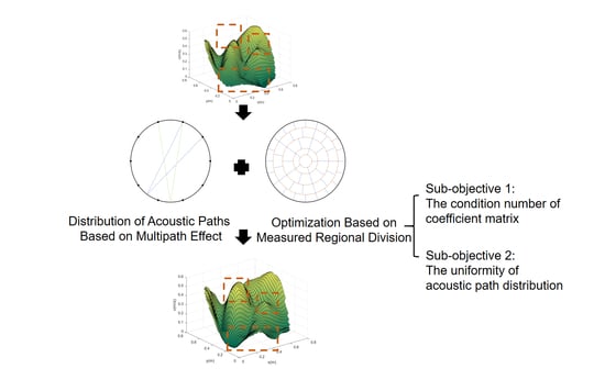
Therefore, to address the above shortcomings regarding the optimization of the transducer topology, this paper proposes a multiple sub-objectives optimization algorithm for measured regional division of acoustic velocity field reconstruction in circular areas.
3.2.2. Design of Optimization Objectives
In terms of optimization objectives, the optimization objectives designed by the method include two sub-objectives, which are the condition number of coefficient matrix A and the uniformity of acoustic path distribution.
In the reconstruction of the flow velocity field, the coefficient matrix
is ill-conditioned, and its degree of ill-health will directly affect the stability of the inversion result. The condition number of matrix is an important indicator to measure whether the matrix is ill-conditioned and the degree of ill-health. For any matrix, the condition number of a matrix
is equal to the product of the 2-norm of
and the 2-norm of
, it is defined as (9):
The larger the condition number, the more severely ill-conditioned the matrix is, which also means that it is more sensitive to small perturbations in the measurement. In velocity field reconstruction, in order to ensure the stability of the inversion results, the measured region division must be designed so that the condition number of the coefficient matrix is as small as possible.
Therefore, in this paper, the condition number of coefficient matrix is used as the first sub-objective for the measured regional division optimization, and the expression is shown in (10):
The smaller is, the lower the degree of matrix ill-conditioning in the inversion is and the better the stability of the velocity field reconstruction results.
In velocity field reconstruction, inhomogeneous distribution of acoustic paths leads to unstable inversion problems and low reconstruction accuracy, and ultimately an imbalance of reconstruction accuracy in different regions within the velocity field.
Therefore, in this paper, the uniformity of acoustic path distribution is taken as the second sub-objective, which is defined as the value of the variance of the length of the acoustic paths passing through all the measured regions with (11).
where
denotes the number of measured regions,
is the sum of the lengths of the acoustic paths through the ith region, and
is the average value of the acoustic path lengths of the measured regions under the current division.
The smaller the is, the more uniformly the acoustic paths are distributed for each measured region, the more complete the flow velocity information of the circular area is sampled, and the better the reconstruction result is.
A total objective function is generated by linearly weighted summation of the above two sub-objectives [
32], as shown in Equation (12):
where
and
are the weight sizes of the two sub-objectives in the total objectives, respectively, characterizing the degree of contribution of each sub-objective to the optimization objectives. Optimization of subregion delineation can be achieved by minimizing E, thus improving the accuracy of velocity field reconstruction.
In this paper, CV is used to solve the weight coefficient of each sub-objective [
33]. CV is a commonly used multi-criteria decision-making method, which determines the weight of each sub-objective by calculating the coefficient of variation of each sub-objective.
CV is a data-based weight determination method, and its basic idea is to determine the weight of each subgoal by calculating its coefficient of variation. The larger the coefficient of variation, the greater the volatility of the sub-objective, indicating that it carries more information. Therefore, a larger coefficient of variation of a sub-objective will lead to a larger influence of the sub-objective on the overall objective, which ultimately leads to a larger weight.
The specific implementation process is described below:
First, by randomly assigning values to the optimization variables, a certain number of samples for the division of measured region are obtained, and the and corresponding to each sample are calculated to make a sub-objective dataset. In order to reduce the influence of outliers on the results, and taking into account that the order of magnitude of the sub-objectives may have a large difference, the dataset was standardized with mean 0 and variance 1, and the mean , , and the standard deviation , were calculated for the standardization of each index.
Secondly, the coefficient of variation is the ratio of the standard deviation of the indicator to the mean, and the coefficient of variation of the two indicators
,
are obtained by using (13).
Finally, the normalized values of
,
are taken as the weights of the corresponding sub-objectives, which are expressed as in (14):
Based on the above optimization variables and optimization objectives, this paper adopts PSO for automatic optimization search for measured region division [
34,
35].
In PSO, each solution to the problem can be viewed as a particle, and each particle has two attributes: velocity and position. The particle swarm algorithm assigns initial positions and velocities to all particles, and in each subsequent iteration, the particles update their velocities and positions by tracking the current optimal position of themselves and the optimal position of the entire particle swarm.
For a d-dimensional particle swarm in the kth iteration, the iterative process is represented by (15):
The in (15) denotes the velocity of the particle in the dimension, and denotes the position of the ith particle in the jth dimension.
denotes the degree of inheritance of the particle to the current velocity, , denote the maximum step of regulation, and , are random numbers between 0 and 1, which increase the randomness of the optimization. A larger is good for jumping out of the local optimum, and a smaller is good for the convergence of the optimization algorithm.


