1. Introduction
Recent technology development in the fields of wireless communication and MEMS has made extensive distribution of wireless sensor networks (WSNs) become possible. It is obvious that WSNs are reliable, accurate, flexible, inexpensive, easy to deploy and have other excellent features. As such, they have potential applications in many areas. For instance, monitoring is one of the most important applications of WSNs, such as the monitoring of agricultural crops, buildings, water quality, etc. These types of sensor networks have the characteristics of centralized data collection, multi-hop data transmission, many-to-one flow patterns, as well as increased data flow brought about by contingency. The above characteristics easily lead to the part or overall congestion of WSNs, which seriously influences the quality of the service of networks [
1]. This can include increased delays in transmitting information and the loss of data packets. It also leads to repeated data sending that further increases the flow of the network, which wastes valuable energy, bandwidth and other network resources.
A traditional wired network [
2] merely affords a transmission platform for data. It adheres to the end-to-end design concept and the intermediate nodes are only responsible for retransmitting data. However, WSNs are different from wired networks in that they are data-centered networks and the intermediate nodes also process data packet; in addition, the physical equipment of the nodes is often subject to destruction and has limited energy. Also, the wireless channel is vulnerable to be interfered with by other transmission signals. All the characteristics mentioned above increase the difficulty of controlling the congestion of WSNs. Therefore, the traditional network congestion control schemes, such as TCP, UDP, etc. cannot meet the requirements of WSNs, which makes the research work on congestion for WSNs more significant and challenging.
Consequently, it is necessary to efficiently control the data transmission of WSNs, which aims at avoiding or properly relieving the occurrence of network's congestion. To be integrated with network congestion and fairness, a cross-layer active predictive congestion control scheme is proposed, which is based on the occupied node memory and data flow trends of local network (grid), as well as combined with network conditions and node rate within period t. It aims at predicting the inputting and outputting rates of node within the next period t + 1 in order to avoid the congestion. The fairness of network and the timeliness of data packets are also taken into account by the design of cross-layer scheme.
The remainder of this paper is organized as follows. Section 2 introduces the related work including typical congestion control protocols. Section 3 provides system architecture and basic models of WSN for later analysis. In Section 4, the proposed scheme is presented in detail, which includes control methods of congestion in node-level and system-level, as well as the revised IEEE 802.11 protocol. Section 5 does the specific analysis based on each performance of CL-APCC. The performance of CL-APCC is mainly evaluated in Section 6. Finally, in Section 7, we make some concluding remarks and outline some future work.
2. Related Work
The growing interest in WSNs and the continual emergence of new techniques has inspired some efforts to design congestion control protocols in this area. Normally, current congestion control protocols in WSNs can be typically classified into two broad categories [
3-
34]: congestion avoidance mechanisms and congestion release mechanisms [
10-
14]. (1) The existing congestion avoidance mechanism is mainly achieved by two kinds of methods. ➀ The first is the rate allocation method [
10,
11]. It requires that the sending rate allocated to the node must be equal to the sum rates which are the rate of generated data by the node and that of all its children nodes. But it is very difficult to allocate the sending rate for each node under the dynamic condition of network topology. Furthermore, if some nodes in the network are not active, bandwidth and other resources of network will be wasted. ➁ The second is the cache notification method [
12-
14] which is passively applied to the circumstances where network congestion has already occurred. In addition, this method can effectively avoid the phenomenon of node-level congestion, however, the system-level congestion (local network congestion) is inevitable. (2) Congestion release mechanism [
15-
34] is achieved by methods of rate adjustment. The weakness of this mechanism is the same as ➁.
Although the two categories above are good for improving network performance, nevertheless, all such methods like (1) and (2) are passive adjustments after the occurrence of congestion (energy and bandwidth have been wasted). In addition, more attention should be paid to address the issues of QoS of network.
The Congestion Control and Fairness (CCF) routing scheme [
10] uses packet service time at the node as an indicator of congestion. However, the service time alone may be misleading when the incoming rate is equal or lower than the outgoing rate through the channel with high utilization. On the other hand, the Priority-based Congestion Control Protocol (PCCP) [
11] rectifies this deficiency by observing the ratio between packet service time and inter-arrival time at a given node to assess the congestion level. However, both CCF and PCCP ignore current queue utilization which leads to increased queuing delays and frequent buffer overflows accompanied by increased retransmissions.
The CODA protocol [
12] uses both a hop-by-hop and an end-to-end congestion control scheme to react to the congestion by simply dropping packets at the node preceding the congestion area and employing the additive increase and multiplicative decrease (AIMD) scheme to control a source's generation rate. Thus, CODA partially minimizes the effects of congestion, and as a result retransmissions still occur. Similar to CODA, Fusion [
13] uses a static threshold value for detecting the onset of congestion even though it is normally difficult to determine a suitable threshold value that works in dynamic channel environments. In both CODA and Fusion protocols, nodes use a broadcast message to inform their neighboring nodes the onset of congestion, though this message is not guaranteed to reach the sources.
The interference-aware fair rate control (IFRC) protocol [
14] uses static queue thresholds to determine congestion levels, whereas IFRC exercises congestion control by adjusting the outgoing rate on each link based on the AIMD scheme. Consequently, the IFRC reduces the number of dropped packets by reducing the throughput. By contrast, the proposed scheme varies the rate adoptively based on the current and predicted congestion level. The control parameters in the proposed scheme are updated according to changing environment, while the IFRC [
14] and others [
12,
13] require that the parameters and thresholds have to be selected before each network deployment.
SenTCP [
15] is an open-loop hop-by-hop congestion control with a few special features. It jointly uses the average local packets service time and the average local packet inter-arrival time to estimate the current local congestion degree in each intermediate node. During congestion it uses hop-by-hop congestion control. But, SenTCP needs strict time synchronization between nodes, which is difficult for WSNs.
In the Event-to-Sink Reliable Transport (ESRT) protocol [
16], a sensor sets a congestion-notification (CN) bit in the packet header if its buffer is about full, which is like the (RT)
2 protocol [
17]. The sink periodically computes a new reporting rate (at which each source is supposed to report data) based on a reliability measurement, the received CN bits, and the previous reporting rate. It then broadcasts the new reporting rate to all data sources. Treating all sources equally is suboptimal. To remove all congestions, the reporting rate has to be set according to the worst hotspot in the network. In that case, the noncongested sources will be constrained by a conservative reporting rate.
As the communication cost from different sources to the sink may be different and may change dynamically, and the contributions of packets from different sources are also different, it is necessary to bias the reporting rates of the sources. But, ESRT adjusts the report rate of sources in an undifferentiated manner. Based on these defects of ESRT, Price-Oriented Reliable Transport protocol (PORT) [
18] employs node price, which is defined as the total number of transmission attempts across the network needed to achieve successful packet delivery from a node to the sink to measure the communication cost. At the same time, PORT dynamically feeds back the optimal reporting rate to each source according to the current contribution of the packets from each source and the node price of each source.
In addition, other protocols [
19-
34] address congestion control from different angles too, but the related works proposed above adopt a passive approach to congestion adjustment. When congestion has occurred in the network, data source control or flow distribution is carried out passively through the feedback. At this point, a lot of useless information has been sent in the network, which results in wasted bandwidth and sensor energy. Naturally, The Active Congestion Control methods [
35,
36] have become particularly important in order to reduce energy overhead and improve bandwidth utilization ratios.
Although the existing schemes play important roles to improve network performance, congestion control is still a challenging area in WSNs. In this paper, an active predictive method based on the research of other relevant protocols is demonstrated. The proposed scheme utilizes the priority of data sending to adjust the inputting and outputting rates of nodes, which prevents the occurrence of network congestion and ensures the timeliness and fairness of data transmission. The difference in our work from the aforementioned approaches mainly includes the following three aspects: (1) In order to actively predict and solve single-node congestion in networks, a single service window with the mixed queuing model M/M/1/m is applied to deal with the issue. (2) The predictive method of periodic flow is adopted to solve the congestion of local networks (grid). (3) The IEEE 802.11 protocol is revised to ensure fairness and timeliness of data transmission in the network by the design of cross-layer (according to the original priority and waiting time of data packets to make sending strategy).
3. Preliminaries
In this section, we describe the system architecture of congestion control protocol and various parameter variable definitions in WSNs. The overall network is divided into grids to better control the congestion of the network. In each grid, the predictive periodic flow method is used to solve the congestion. The basic grid models are illustrated for later analysis, including definition of each period length, selection of node with flow predictive feature (named A-type node) and the status of how to deal with failure of an A-type node in each grid.
3.1. System Architecture
Here, we consider a scenario where the WSN is formed by stationary sensors in a two-dimension
R2 sensing field. In order to better control congestion of local network, there are several main parameters to be set. The whole of
R2 space is divided into the grids number,
K, and each grid is deployed in a square with the length of side,
h. So the grid number
K = (
H ×
H)/(
h ×
h), the value of
k increases in turn from left to right, and the grid value of the lower level is often bigger than that of the upper level (as shown in the
Figure 1). Nodes are intensive enough and randomly distributed. The initial energy of each node is homogeneous and can not be complemented. The communication radius of the node is
r, and the aim of
is to ensure each node in the same grid can normally communicate. Each node knows its initial position. Sensors periodically report the information about the monitored events to BS. For each node, any other node in its communication range could become its neighbor.
In order to further to demonstrate the node and packets of the network, it is necessary to demonstrate the node i. The coordinates of i are v(Xi, Yi), so according to the initial position, the grid value of the node i is ki = [Yi/h] × (H/h − 1) + [Xi/h], and the number of i's neighboring node is
. The length of the data packet is
. The packet header structure of node i in grid k is:
, among which the variable of ParentIDSi is a direct upstream neighboring set of node i (near to the BS) and the variable of ChildIDSi which is a downstream neighboring set of node i (around the data sources). These two variables are decided by the specific routing algorithms.
and
which respectively represent the inputting and outputting rate of node i in period t.
and
are separately expressed average inputting and outputting rate of grid k, and the last variable of Eni(t) represents the current residual energy of node i.
3.2. The Grid Structure
In order to better control congestion of a local network, the whole network is divided into grids. In each grid, the predictive method of periodic flow is adopted to solve local congestion. The detailed demonstration of the grid structure is illustrated below.
First, we explain how to select the A-type in each grid. A node is randomly selected as the A-type node in each grid during the initialization of the network. In the operation process of the system, the packet header of the node has its own residual energy information Eni(t) (we describe the packet header structure of the node in subsection 3.1). In order to better explain this issue, we assume that the current time of grid k is in period t and the A-type node is Ak(t). Residual energy Eni(t) of node i in the packet header was monitored by Ak(t). At the end of period t, a new A-type node (Ak(t + 1)) from the next period t + 1 is changed into the node which has the maximum residual energy (Max(Eni(t)) in the grid. At the same time, Ak(t) broadcasts the new A-type node (Ak(t + 1)) to all nodes in the grid.
Second, the period of each grid is described. The A-type node has been set to promiscuous mode to monitor all nodes in the grid. Once the A-type node has monitored that all nodes in the grid have already sent data one time, then it broadcasts to the other nodes in the grid that this period is finished and notices which node becomes a new A-type node in the next period. Concurrently, a new period begins and the new A-type node starts to monitor the data flow of the grid under promiscuous mode in the new period.
Third, it is illustrated what to do if the A-type node fails. The period of each grid has its own maximum time Max(t) (Max(t) is described in subsection 5.1). Hence, each node maintains a counter to reflect the broadcast signal of the A-type node in the grid. If the node doesn't receive the broadcast signal from the A-type before the maximum time of its own grid, then the node believes that the A-type node has failed. The data sending sequence of the node which ranks first place in the grid (there will be illumination about the data sending sequence of the nodes in Section 4.2) will temporarily be used as the A-type node. Concurrently, the temporary A-type node broadcasts itself to all nodes in the grid. In the next period, the A-type node is still chosen to be the node which has the maximum residual energy in the grid.
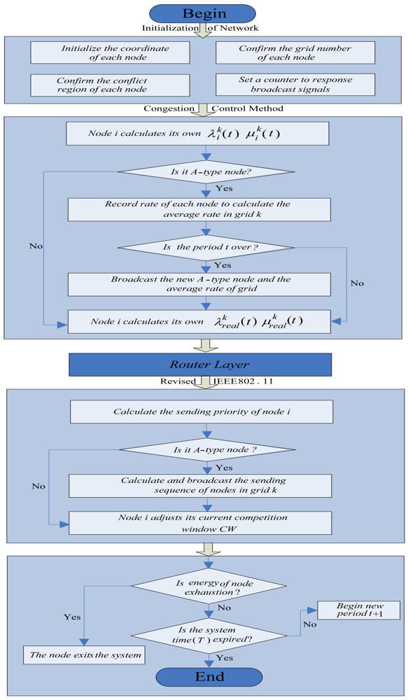
4. CL-APCC Protocol
Congestion is mainly caused by two factors. First, data is received too quickly, which leads to the overflow of the node. Second, a great deal of collisions occur between data packets which are sent by nodes. Hence, according to periodicity reports or data flow characteristics of application types such as emergency monitoring, we separately analyze the existence probability of node-level congestion and local congestion(system-level) in the network in order to overcome the node overflow. The probability of congestion is analyzed to dynamically adjust the receiving and sending rate of nodes. Consequently, the IEEE 802.11 protocol is revised, which is designed to reduce the collision probability of packets and guarantee the fairness of network transmission. Normally, CL-APCC is divided into two steps. (1) According to the node memory size, the scheme adopts a single service window of the mixed queuing model M/M/1/m to predict and solve the node-level congestion. Then, according to the average inputting and outputting rate of the grid and the status of occupied node's memory size in the period t – 1, the CL-APCC predicts the grid's probability of congestion within the period t. In this way it controls the average inputting and outputting rate of the grid based on the probability of congestion. This solution is used to solve the congestion of local networks (system-level). Finally, according to the adjustment method of node-level and system-level, the real sending rate of node is set to solve the congestion of the entire network. (2) The IEEE 802.11 protocol is revised in the foundation of the first step, which is aimed to guarantee the fairness of network and the timeliness of data packets. The design principle of this protocol is described below.
We adopt the modular mechanism from the top to bottom to describe the data flow in any node. Node
i is analyzed in a certain grid
k. Firstly, it is an initialization module which includes the initialization of the node coordinate, the grid number of the node, the conflict region of the node and the initial rate of the node. Secondly, it is a congestion control module. In this module, node
i first calculates its own inputting rate
and outputting rate
in period
t according to the node-level congestion control method. Next, if node
i is not an A-type node, it is necessary that node
i immediately calculates its real rate
and
. On the contrary, if node
i is the A-type node, it records the rate of each node in grid
k for the calculation of the average rate in period
t + 1. At the end of period
t, node
i broadcasts what is the new A-type node and the average rate of grid
k. Thirdly, data stream flows into a routing layer and from there it flows into the lower layer (the specific routing layer is not taken into account in this manuscript). Fourthly, the data stream flows into the revised IEEE 802.11 module. In this module, at first, it is calculated in the first slot for the sending priority of node
i. Then it is analyzed whether or not the node is an A-type node. If so, node
i records and broadcasts the sending sequences of all nodes in grid
k. On the contrary, if node
i is not the A-type node, with the increase of times that node
i competes for channels, the CW gradually decreases, which gives the node a higher probability of acquiring the current slot. The final module is the one which is determined by nodes whether or not they exit the system (see
Figure 2 for the data flow in any node)
4.1. Network Congestion Control Methods
Congestion has local relevance. That is, congestion would normally appear in a number of nodes in the local network. Furthermore, the control method of node-level congestion cannot entirely reflect the real status of a network. Therefore, CL-APCC respectively analyzes a single node and the data flow of the grid where the node lies. Based on the analysis, the rate control method is adopted in advance to avoid congestion occurring.
Here, a simple description is made to introduce the congestion method of the node-level and system-level. Assume that the occupied node memory size is
L, the maximum node memory size is
m, and threshold value is
Lmax [
15]. Firstly, we describe the congestion control method of the node-level. If the occupied node memory size is
L <
Lmax, CL-APCC identifies the node isn't congested. If the memory size is
Lmax <
L <
m, then CL-APCC identifies the congestion of node-level to have probably occurred. In this case, the sending rate of the node is adjusted to control the congestion. If the occupied node memory size reaches the maximum(
L =
m), the input rate of the node is adjusted to 0. Secondly, we describe the congestion control method of the system-level. At the beginning of a new period
t, CL-APCC protocol makes a prediction for the expected value
E(t) of data quantity in period
t using the average rate in period
t – 1 in the grid. If
E(
t) <
n ×
Lmax(
n is the number of nodes in the grid), congestion of system-level does not occur. On the contrary, if
n ×
m >
E(
t) >
n ×
Lmax, congestion of system-level may occur. In this case, the average inputting and outputting rates of the network are adjusted to avoid system-level congestion (because we strictly control the margin between the inputting and outputting rate, it could not occur
E(t) >
n ×
m).
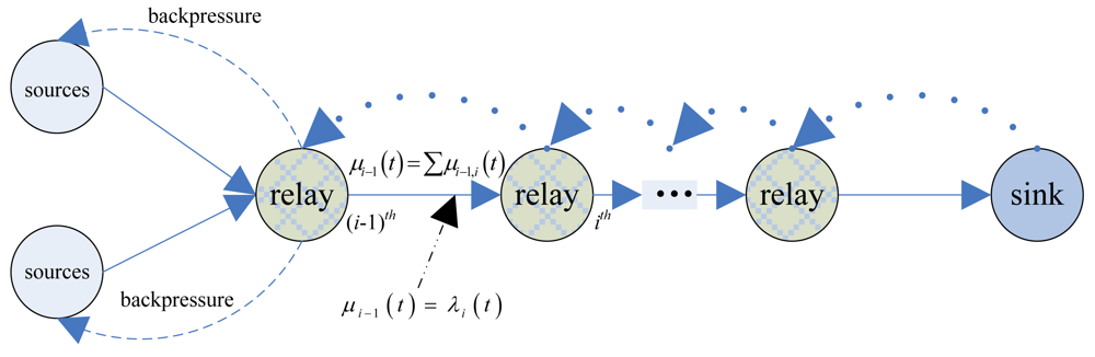
In practical applications, according to the status of network resource, CL-APCC separately sets a weight for node-level and system-level to obtain the real rate of each node. Assume that the total outputting rate of the upper nodes is equal to the inputting rate of the lower nodes. This means that the outputting rate of node
i is decided by the inputting rate of node
i + 1. Each node obtains its data retransmission rate according to the relationship between inputting and outputting (the model of the sending rate is shown in
Figure 3).
Now, the congestion methods of the node-level and system-level are described in detail below. Node i is analyzed in a certain grid k.
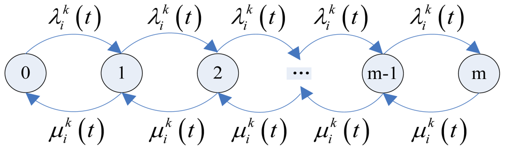
4.1.1. The pre-control and adjustment method of node-level rate
It is better to adopt a single service window of the mixed queuing model M/M/1/m [
38] to make an analysis of the inputting and outputting rate of each node because of the limited memory size. The stable state of the queuing model is shown in
Figure 4.
It can be seen from
Figure 4, the stable state model Equation as follows:
By the regularity conditions reduced.
According to the analysis of telecommunications network model [
39,
40], if
ρ ≤ 0.6, the quantities of data packets are slowly increased in the network, and then the system gradually achieves the optimal state. If
ρ > 0.6, the system quickly reaches the saturation state which leads to data packets badly overflowing. Thus, the sample rates of data sources based on data requirements of the BS in unit time can be obtained as well as the constraints of
ρ value. Also, from literature [
15], the node may appear congested in the WSNs if a node's occupied memory size is larger than a threshold
Lmax. Therefore, the total congestion probability of the node occurred as follows:
namely:
From
Equation (5), we can see the relationship between
ρ, occupied node memory size
L and the congestion probability of the node. Thus, the retransmission rate of intermediate nodes can be obtained according to the data quantity requirements of BS.
Assume that occupied node memory size is
L (
m >
L >
Lmax), therefore, its congestion probability is as follows:
To correspondingly reduce the value of
ρ:
We discuss the changing status of the node's rate from two aspects based on the adjustment of ρ. ➀ After some time, if the occupied node memory size L regains access to the optimal interval, namely L ∈ [0,Lmax], then the value of ρ is maintained unchanged (If ρ is adjusted to 0.6, this leads the node back to the state of congestion and consequently cause frequently oscillating). ➁ If L = m, the inputting rate of node i is set to be 0, namely
. That is because the channel from node i to i + 1 may experience large scale fading (the period length of large scale fading is
, the further detail to explain this issue has been discussed in the next paragraph), it is necessary for node i to lose packets, so CL-APCC protocol sets node i to lose the data packet which has the lowest priority (we will discuss the issue of priority in subsection 4.2).
Node i notifies node i – 1 through an ACK message, and then node i – 1 sends feedback “ACK” to node i – 2 and iterates it to data sources which correspondingly reduce the sampling frequency. Node i is trying to send data after a random period of time (the length of random time is set to be the value between
and
, which is decided by the period length of large scale fading.). If possible, node i first send data at the maximum rate. If the occupied node memory size regains access to the optimal interval, then the node i adjusts ρ = 0.6. Meanwhile, node i notifies node i – 1 using ACK message and the message is iterated to the data sources.
Here, we describe the reason that the period length of large scale fading is not
but
. In the network, it is seen that the earlier large scale fading is found, the better the results. Because it can not only save the energy of network, but also avoid the waste of bandwidth. Under ideal conditions, it is better that the large scale fading can be found once it has occurred. So, it seems that the period length of large scale fading should be
. Nevertheless, we set the period length of large scale fading is not at
but
. The reason is detailed as below: If the state of L = m has been continued a time of
, it means at that time the node i is in the state of sending data but not really sending out. In other words, node i makes analysis for its storage state while data is just being sent, which leads the node to make errors because of congestion caused by itself. So, the typical period of large scale fading is
.
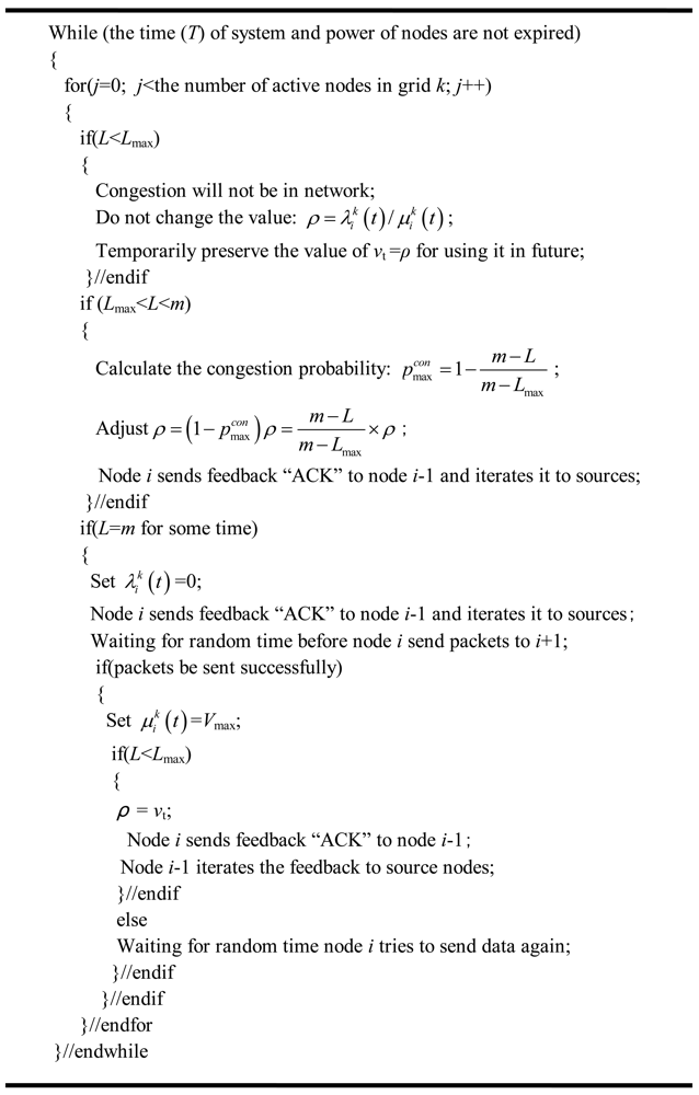
In conclusion, the congestion can be effectively unblocked using
Equation (7) as well as the ACK messages when the node may experience congestion (the pseudo-code is shown in
Figure 5). But all of the above congestion problems only consider the perspective of the node-level. Owing to the occurrence of network congestion with the characteristic of space relevancy, solutions must be obtained to unblock congestion both on the node-level and system-level.
4.1.2. The pre-control and adjustment method of system-level rate
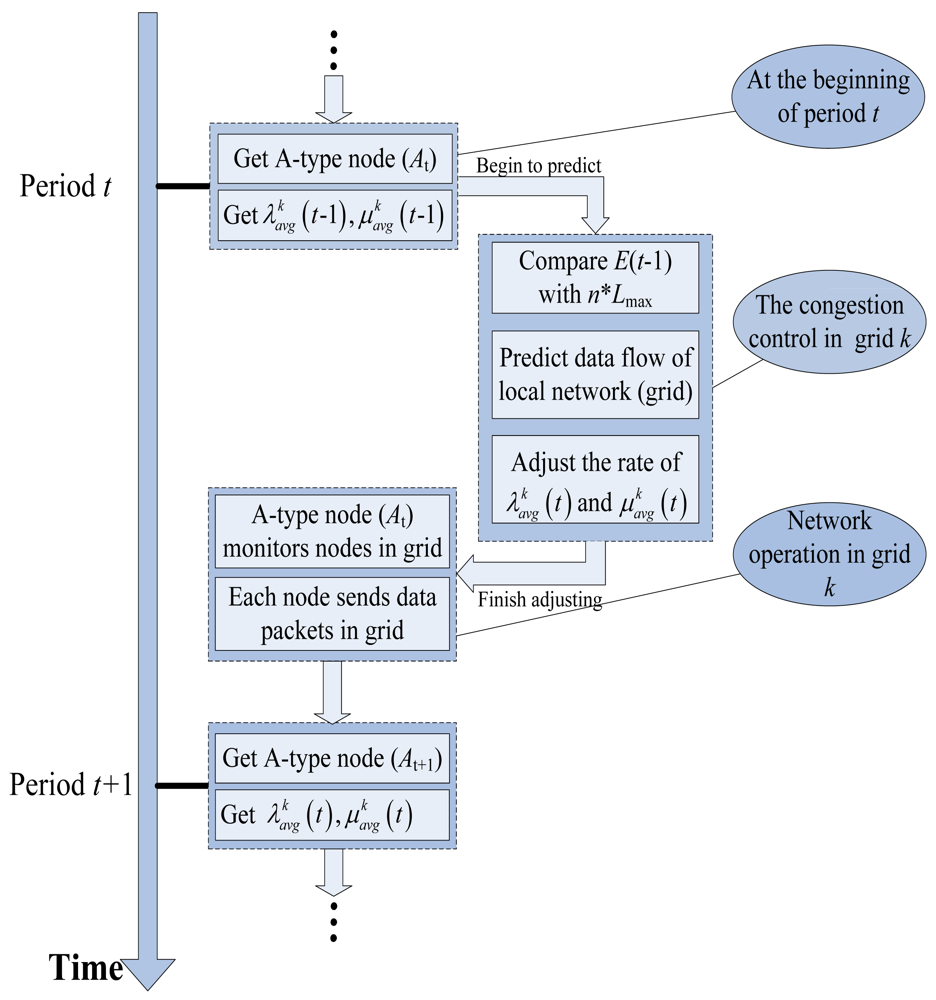
Now, we describe the system-level congestion control in detail (see
Figure 6 for the flow chart of the system-level control method). Node
i is analyzed in a certain grid
k. (The grid structure, period and A-type have been described in subsection 3.2). The A-type node has been set on promiscuous mode to record the rate
of the node
i in grid
k for average rate calculation
. In order to conveniently adjust the average rate according to the local occupied memory resources
E(
t – 1), as well as the average inputting and outputting rates in the previous period
t – 1, CL-APCC predicts the occupied memory resources
E(
t) in period
t and uses the relationship between
E(
t) and
n ×
Lmax, as well as the ratio of
E(
t) and
E(
t – 1) to decide the adjustment method of the average inputting and outputting rates in period
t, which avoids the occurrence of local congestion.
At the beginning of the period
t, it is assumed that the number of nodes to transmit data in grid
k is
X(
t) =
n < N/k and the average rate is
,
; if ➀ The probability that data inputted to grid
k is in direct ratio with Δ
t, recorded as
bn × Δ
t, inputting two or more data with a probability that is
O(Δ
t), ➁ The probability that data outputted from grid
k is in direct ratio with Δ
t, recorded as
dn × Δ
t, outputting two or more data with a probability that is
O(Δ
t). In order to analyze the change of the data quantity in the grid, it first needs to get the mode of
Pn(
t) [
41] which means that the event probability can be decompounded as:
If X(t) = n – 1, input only one quantity of data in the grid within Δt, so the probability is Pn-1(t) × bn-1 ×Δt;
If X(t) = n + 1, output only one quantity of data in the grid within Δt, so the probability is Pn+1(t) × dn+1 ×Δt;
If X(t) = n, there is not any inputting and outputting data in the grid within Δt, the quantity of data hasn't changed, so the probability is Pn(t) × [1 – dn × Δt – bn × Δt],
According to the full probability Equation, we can see that:
The differential Equation of
Pn(
t) is:
Equation (10) is very complicated and with no easy solution value. Actually, we are only interested in the expectation value
E(
X(
t)) (namely
E(
t)) and variance of
D(
t). Owing to the fact that
N can choose any value in theory, in order to conveniently discuss the continuously changing characteristics of the quantity of data, we take the limitation value as the approximately true value that is meaning to assume
n → +∞. The expected value of data derived from the
Equation (10) is:
The changing expectation value in the grid derived from
Equation (14):
The other expression of E(t) is as below.
(proved by Theorem 4 in the Section 5.4)
The changing proportion of storage quantity in the grid is as below:
If 0 ≤ E(t) ≤ n × Lmax, the average rate keep period t-1 unchanged. If n × m > E(t) < n × Lmax,
be decreased as below.
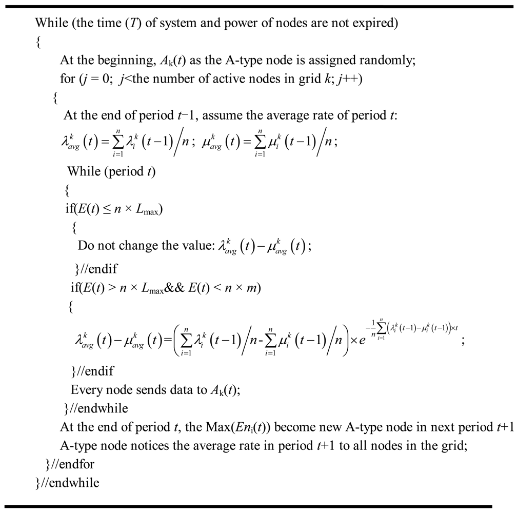
It results that the adjustment equation of the average rate in the grid from
Equations 17 and
18, which can avoid the local congestion of the network through the adjustment method. The pseudo-code is shown in
Figure 7.
4.1.3. The calculation method for real rate of each node
According to subsections 4.1.1 and 4.1.2, it is considered both from the node-level and system-level, which expresses the real rate of the node as below.
The inputting rate of node in period t.
The outputting rate of node in period t.
In sum, the pre-control rate of the node-level is combined with that of the system-level to control congestion, which takes into account the relationship between one part and the whole of the network. In the practical application, CL-APCC protocol increases the value of weight α when bandwidth and channel quality is in the higher proportion to effectively use the network resources in the whole. Whereas, CL-APCC protocol decreases the value of weight α when the retransmission quantity of a certain node is lower and its child-node is less, which is aimed to make the node effectively use its own resources (such as storage space and rate, etc.) to obtain the highest efficiency of the network in the whole.
4.2. The Revised IEEE 802.11 Protocol of CL-APCC
In this section, the IEEE 802.11 protocol is revised in order to decrease the transmission conflicts of data packets and ensure the fairness and timeliness of networks. In the network, there are different requirements of multi-data flow on reliability and sending timeliness, so it is necessary to have a priority control strategy in WSNs. In this paper, according to the sending priority and he service time of packets at the node, CL-APCC protocol makes a rule on how to deal with the priority of data packets.
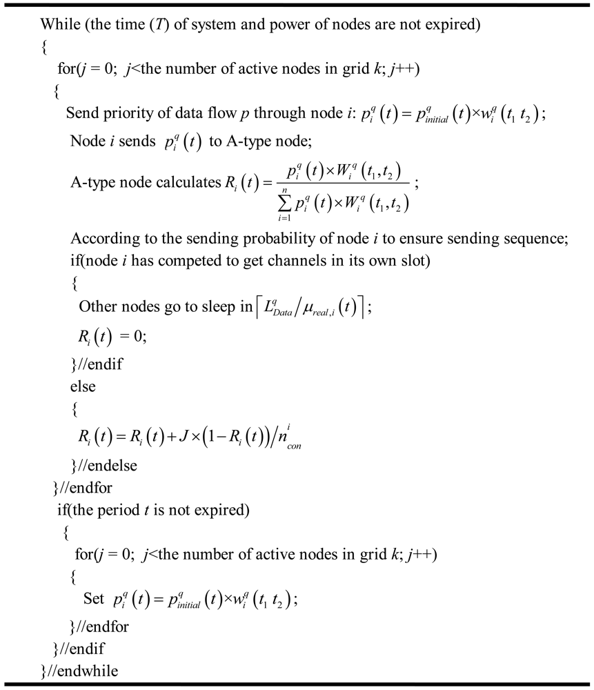
First, the revised IEEE 802.11 protocol method is described in general. The CL-APCC protocol dynamically adjusts the current competition window (CW) of a node based on the original priority and the service time of packets at the node. As the times of node's competition channel increase, the size of CW gradually decreases and accordingly results in an increase in the probability which acquires the current slot. Once the node competes to obtain slot in period t, then its competition probability reduces to the minimum (CW = βCWmax) till the end of the period t.
Next, we describe the revised method of the IEEE 802.11 protocol in detail as follows:
Node
i is analyzed in a certain grid
k. Assume the waiting time is
which means packet
q service time at the node
i, the length of packet
q is
, the original priority of packet
q is
. So the sending priority of this packet is calculated as
. According to the feature of sending priority of packets, node
i takes
as a packet to be sent. At the beginning of period
t, node
i sends the value of
to the A-type node in the grid. After the integrated calculation of the A-type node, it can be obtained the sending probability of node
i in the first slot as
Equation (21). Concurrently, the A-type node notices the sending sequence of nodes to all nodes in the grid. Furthermore, each node maintains a counter to remember the sequence for the calculation of its sending probability and to deal with A-type node failure (as described in subsection 3.2).
It will be divided into two situations to discuss the sending probability of node
i: ➀ if node
i can compete to obtain a sending slot at its own moment, then
Ri(
t) = 0, the other nodes in the grid will switch into the sleeping state in the next
slot to save energy. When node
i finishes sending a data packet, the other nodes in the grid begin to compete for the channel. ➁ If node
i doesn't compete to obtain the channel at the moment, it competes again after the node which has already competed to obtain slots and finished sending data. The sending probability of node
i is updated as below:
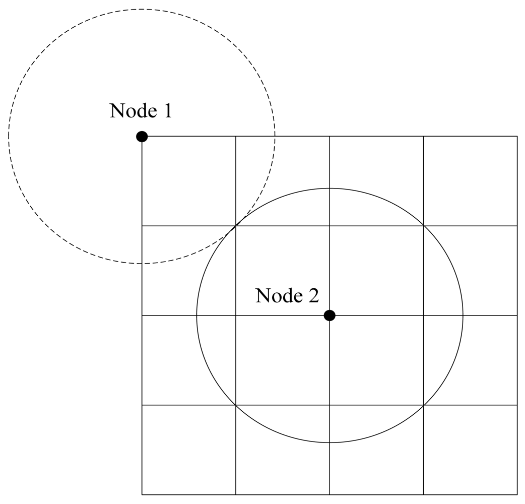
J is competition times and
is neighbor quantity in the communication range of node
i (each node's value of
is different), it can show the scope of
in
Figure 8.
At the end of the period
t, the A-type node in the grid turns to the next period of calculation for the average rate and node sending priority. The pseudo-code is shown in
Figure 9.
7. Conclusions
Congestion has a severe influence on network performance, which results in a large number of missing packets, unfair status of network and significant wasted energy due to the repeated sending packets. Focusing on the problems, we propose a cross-layer active predictive congestion control protocol (CL-APCC) for WSNs. The basic concept of the CL-APCC protocol is described as below.
Each node adopts a single service window of mixed queuing model M/M/1/m to predict and resolve node-level congestion. CL-APCC predicts the probability of congestion caused by the grid in period t, and the probability is used to control the inputting and outputting rate of the grid, which effectively solves the system-level congestion problems of the network. Therefore, the congestion is solved through the combination of node-level control method and system-level control method. At the same time, the IEEE 802.11 protocol is revised in CL-APCC to meet the requirement of fairness of networks, which is depending on the service time at the node and original priority of data packets. We make a complete analysis and simulate on the proposed scheme, which shows that it exceeds other methods relying on not only RPR and lifetime of network but fairness and timeliness of data packets.
However, the kind of congestion control protocols under the circumstances where nodes can be moved have not been considered. Still, we have not yet found an optimal method to set communication radius for the node. Nevertheless, such issues are to be studied in the future so that CL-APCC protocol has much wider applications.


