2. Sensor Modelling
In previous research, three approaches were used to determine sensor output modelling. The models are the optical path length model, optical attenuation model and optical path width model. Ruzairi [
1] first applied the optical path length model in his work to predict amplitude of sensor output voltage, which resulted in a proportional relation between the output voltage amplitudes and the particle flow rate. Research by Ibrahim
et al. [
2] has shown that the optical attenuation model is suitable for use in liquid/gas systems where both media are transparent but possess different optical attenuation coefficients. Chan [
3] has investigated the two previous optical models and concluded that both models are unsuitable for his project, which applies light intensity measurements and uses solid particles as flow materials. In his deduction, he concluded that the signal conditioning system that employs light intensity measurement is not suitable for the optical path length model and that solid materials used as flowing objects have high absorption characteristics which make use of the optical attenuation model unsuitable as this kind of model must assume both conveyed and conveying mediums are transparent. Thus, this research adopts the optical path width model applied by Chan
et al. [
4] where sensor modelling is done based on the width of the sensing beams within the pipeline projections. Generally, the basic principle of the sensor modelling in this project is light beams transmitting in a straight line to receivers [
5]. The sensor output is dependent on the blockage effect when solid materials intercept the light beam. As the first step to approach the sensor modelling, a few assumptions are made to obtain the model. The assumptions are as follows:
According to Chan [
3,
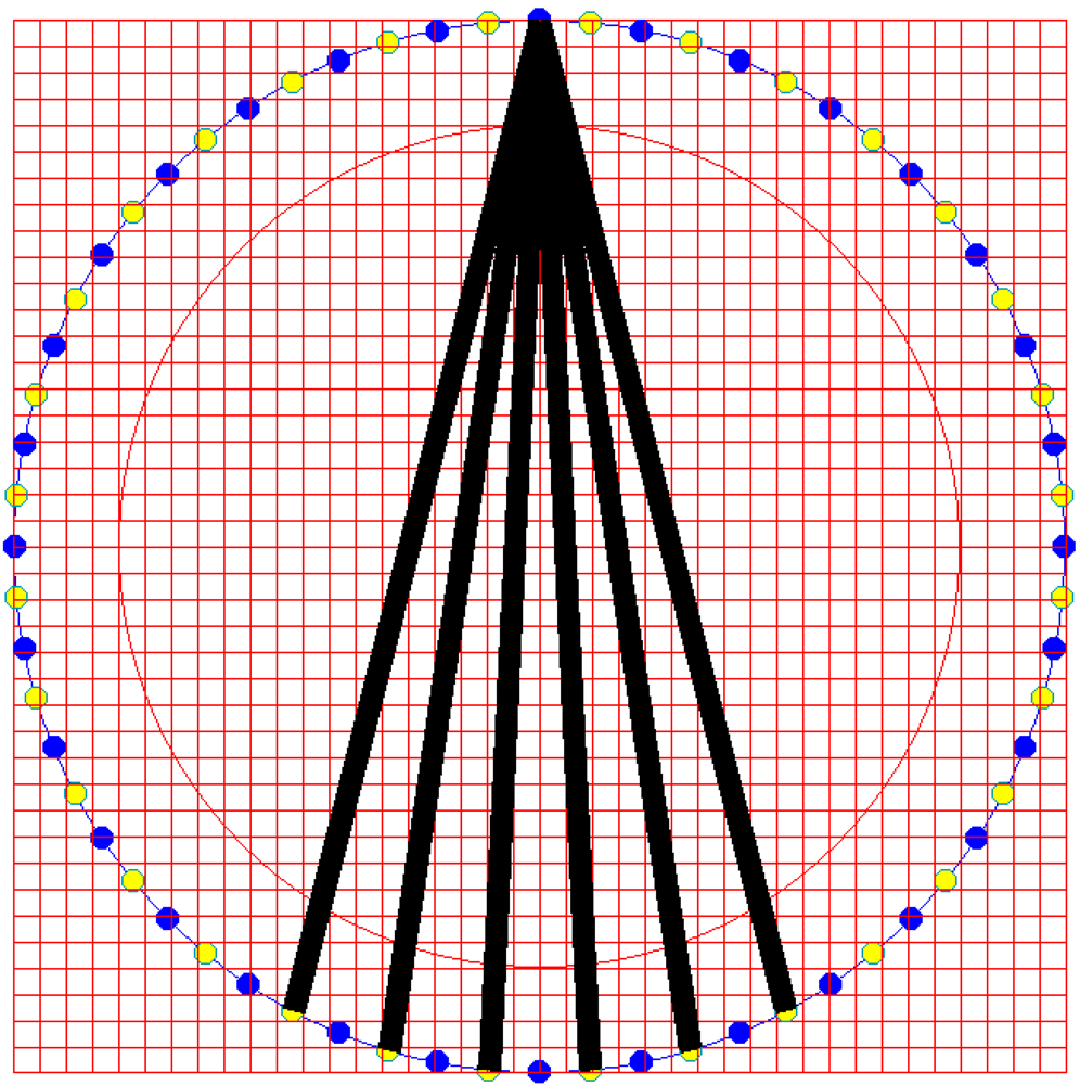
7], the width of each beam is dependent on the angles of the light that arrives at the corresponding receivers. His application involves the transmitter's single emission which is received by all the receivers in the pipeline. However, in this multiple fan beam projection application using optical fibre sensors, the width of the light beam is small and the transmission angle of the transmitter is 30 degrees where only six receivers will receive light from one transmitter, as illustrated in
Figure 2.
The width of each beam is considered constant along the emission towards all the corresponding receivers by using the tangent approach. This approach is taken based on the investigation on Chan's modeling [
3,
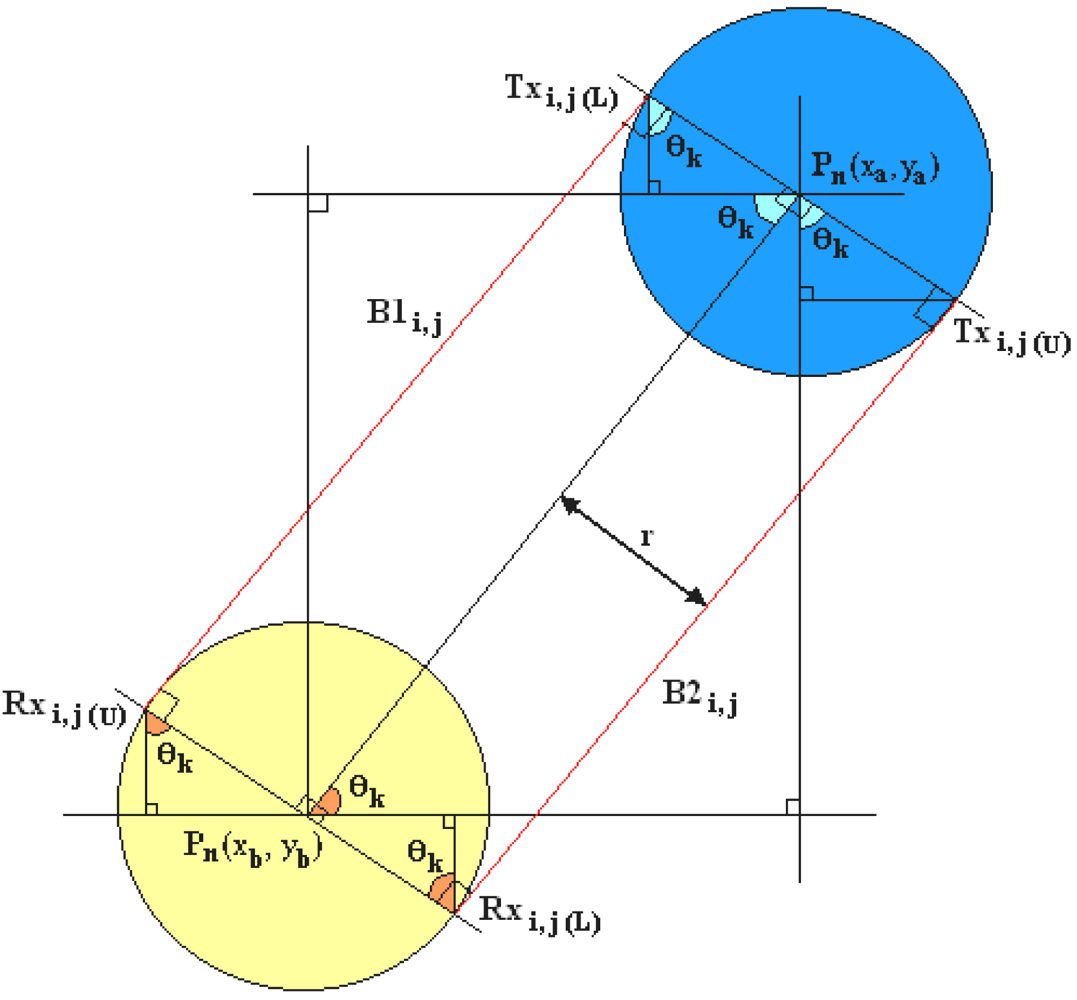
7]. It is found that the width difference of light beams from one transmitter to the corresponding receivers affected by the transmitting angle of 30 degrees is very small (±4% or ±0.1mm difference). Based on this calculation and to make the modelling in Visual C++ programming easier, the tangent modelling of the sensors is as shown in
Figure 3.
From
Figure 3, P
n(x, y) is the centre of the sensor's coordinates. After mapping the transmitters and receivers onto the map with a scale from (0, 0) to (640, 640), there is a need to simplify the boundary determination for each emission light from emitters to receivers [
3]. B1
i, j and B2
i, j are the border lines of the light path while Tx
i, j (L), Rx
i, j (L), Rx
i, j (L) and Rx
i, j (L) are the coordinates which forms a polygon to satisfy the boundary points.
For different sets of transmitter and receiver's light beams, there are different sets of boundary points/coordinates. Firstly, θ
k must be calculated with
Equation 1:
where
θk = the angle needed to find boundary coordinates,
ya = the y-th coordinate of the n-th transmitter,
xa = the x-th coordinate of the n-th transmitter,
yb = the y-th coordinate of the n-th receiver and
xb = the x-th coordinate of the n-th receiver.
Once the centre coordinates, P
n(x, y) and θ
k have been obtained, the boundary coordinates can be determined with
Equations 2-
9:
where
r = radius of the sensor which is 7 pixels,
i, j = the beam for i-th transmitter and j-th receiver,
Txi,j(L) x = the x-th coordinate of the lower boundary of corresponding transmitter,
Txi,j(L) y = the y-th coordinate of the lower boundary of corresponding transmitter,
Txi,j(U) x = the x-th coordinate of the upper boundary of corresponding transmitter,
Txi,j(U) y = the y-th coordinate of the upper boundary of corresponding transmitter,
Rxi,j(L)·
x = the x-th coordinate of the lower boundary of corresponding receiver,
Rxi,j(L) y = the y-th coordinate of the lower boundary of corresponding receiver,
Rxi,j(U) x = the x-th coordinate of the upper boundary of corresponding receiver and
Rxi,j(U) y = the y-th coordinate of the upper boundary of corresponding receiver.
In order to obtain a connection between the sensors and solid particles that intercepts the light beams during several flow conditions, the optical path width model is being applied. Only one modelling approach is needed to generate the sensor outputs for light interception of solid particles with different sizes and shapes. Prior to this, the upper and lower boundary points have been found. On the same image plane, the light beams for all the corresponding transmitters and receivers are being drawn. In the situation of six receivers receiving light from one transmitter, the total of light paths in one frame of light emission is 192. Each light beam is in the form of straight line, therefore there is a gradient for every light path according to the linear graph equation. The gradient here means a number that represents the steepness of a straight line. By using the boundary points, the gradients of the light paths can be obtained as referred to
Equation 10:
where
mi,j = the gradient/slope of light path for i-th transmitter and j-th receiver,
Rxi,j(U) y = the y-th coordinate of the upper boundary of corresponding receiver,
Txi,j(L) y = the y-th coordinate of the lower boundary of corresponding transmitter,
Rxi,j(U) x = the x-th coordinate of the upper boundary of corresponding receiver and
Txi,j(L) x = the x-th coordinate of the lower boundary of corresponding transmitter.
The next step is to investigate the sensor output condition if the light path is being intercepted by solid particles. The particles might intercept the light beams in many different ways, for example fully or partially blocking the light path. By using the linear graph extrapolation method, the ‘y intercept’ of each boundary lines for all possible combination of transmitters and receivers are attained by following
Equation 11 and
Equation 12. Here, ‘y intercept’ means the y coordinate of where the straight line graph cuts the y-axis:
where (
0,cB1i,j) = the ‘y intercept’ of the first border line for the i-th transmitter and j-th Receiver while (
0,cB2i,j) = the ‘y intercept’ of the second border line for the i-th transmitter and j-th receiver.
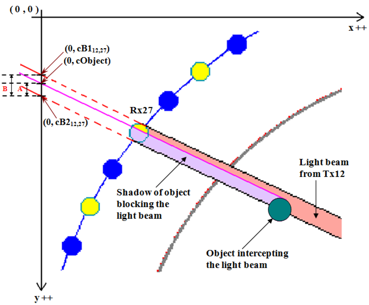
Basically in modelling, an object is formed by pixels as well.
Figure 4 shows an example of an object intercepting a light beam from T × 12 to R × 27. To find out the sensors condition when an object blocks the light beam, each of the pixels that forms the object has to be extrapolated to find the ‘y intercept’ of that particular pixel using all the possible combinations of gradients found in
Equation 10. By using Visual C++ programming, the ‘y intercept’ value of the object labelled as (0, cObject) in
Figure 4 is obtained dynamically, which means this value will vary when processed with different gradient values. If the ‘y intercept’ of the pixels that form the object lie in between the first (0, cB1
ij) and second (0, cB2
ij) extrapolated ‘y intercepts’ of any corresponding light paths, the ratio of the intercepting pixels to the width of the light beam is being calculated.
However, if any of the ‘y intercept’ for pixels formed by the object has the same value, this value is only counted once and the rest are ignored. ‘
A’ in
Figure 4 summarizes the shadow of object blocking the light beam while ‘
B’ is the total pixels area of the light beam as referred to when x-axis is zero as reviewed in
Equations 13,
14,
15,
16 and
17.
where:
Z(x,y) = all the possible coordinates of the pixels which form the object, obtained using programming looping to retrieve the colour of the pixels (drawn with green colour to represent the object). The range of x and y of Z(x,y) are 64 ≤ x < 576 and 64 ≤ y < 576.
cObjecti,j = all the possible ‘y intercepting’ of objects for i-th transmitter and j-th receiver.
Z.y = the y-th coordinate of the possible object pixels obtained in
Equation 13.
Z.x = the x-th coordinate of the possible object pixels obtained in
Equation 13.
mi,j = all the gradients for i-th transmitter and j-th receivers attained in
Equation 10 pi,j = an array to store the frequency of ‘y intercepting’ of objects which fulfil the given conditions where 1 is when the ‘y intercepting’ of object falls in between the border lines of the light beam for a particular i-th and j-th light beam; and it is 0 when the conditions are not fulfilled. Since the object vary in size, it is also possible that the more than one of the Z(x,y) pixels has the same cObjecti,j in a single light beam. If this happens, this value is discarded or equals to 0.
cB1i,j = the ‘y intercept’ of the first border line for the i-th transmitter and j-the receiver.
cB2i,j = the ‘y intercept’ of the second border line for the i-th transmitter and j-the receiver.
Bi,j = a counter to sum all ‘y intercepts’ of object pixels obtained in
Equation 15 according to the i-thtransmitter and j-th receiver.
Ai,j = the width of the light beam for i-th transmitter and j-th receiver when it cuts the y-axis at x-axis equals to zero.
In order to predict sensor values for various flow models,
Equation 18 is applied:
where
Vi,j = the predicted sensor output for i-th transmitter and j-th receiver,
Vrefi,j = the assumed voltage reference for i-th transmitter and j-th receiver. As said earlier in this section, this modelling uses the tangent method to model the sensors, thus the light beams have a constant and it is equals 5 volts in this case.
3. Sensitivity Maps
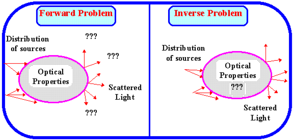
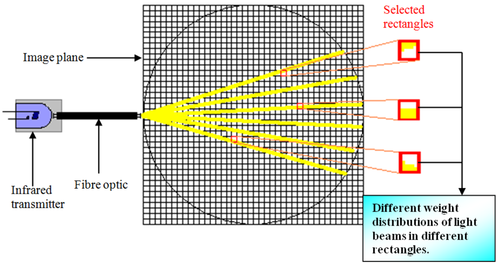
From the fan beam projection properties, it is known that the fan beam projection can be seen as a point source of radiation that emanates a fan shaped beam. The emanation covers many directions in different angles. For a given source and detector combination, functions are calculated that describe the sensitivity of each source and measurement pair to changes in optical properties within each pixel of the model [
8]. Thus, when the projection beam is mapped onto the two-dimensional image plane, each light beam will spread across each rectangle in different weights, as illustrated in
Figure 5.
The solution of the forward problem generates a series of sensitivity maps, and the inversion of these sensitivity matrixes therefore provides a reconstruction of the optical properties [
8]. Basically, the number of generated sensitivity maps is dependent to the number of projections for the sensors. No matter whether the applied projection method is the 2-projection or 4-projection method, each light beam must be sampled individually. Therefore, for the thirty-two transmitters and the corresponding six receivers which receive light per emission of each transmitter, the total projections are 192. This means that there will be 192 sensitivity maps generated as well. Before these sensitivity maps can be used for image reconstruction, they must first be normalized.
Normalization of sensitivity maps is done when there is no simple linear relationship between the weight distributions in a rectangle for different light projections. For example, the rectangle (25, 30) might have certain percentage of light passing through for the light beam of transmitter 10 and receiver 25. When transmitter 0 emits light to receiver 16, this light beam might pass through rectangle (25, 30) with a different weight distribution. If there are other light beams passing through the same pixel as well, the weight distribution of the pixel will become complicated. Thus, it is necessary to build a general relationship between the pixels and all the projection beams that pass through the pixels. A simple approach to normalize the rectangle values in this research is engaged in a similar manner as normalizing the pixel values in ECT so that they have the values of zero and one when the rectangle contains the lower and higher weight distributions respectively.
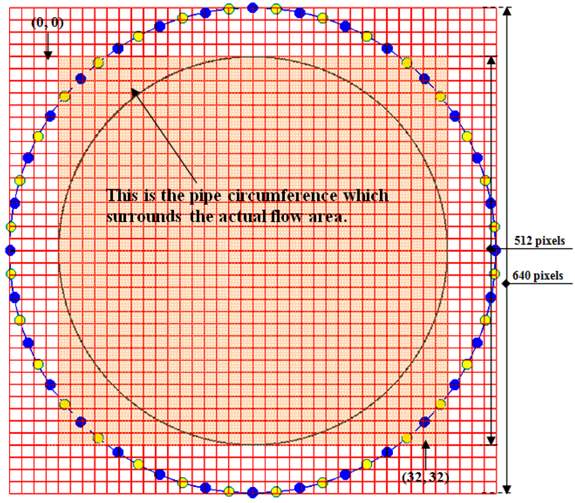
As a reference to map the sensitivity maps onto the 2-dimension image plane, see
Figure 6. From the 640 × 640 pixels plane, there are gridlines to divide the pixels into 40 × 40 rectangles where each rectangle contains 16 × 16 pixels. In image reconstruction, the actual area of flow is from pixel 64 to pixel 575 in the x-axis and y-axis. In this section and the following section, the image plane is reconfigured so that all calculations and scanning of pixels are done only for the part of the actual flow area. This is being done to avoid wasting unnecessary time and resources used to calculate and scan the whole 640 × 640 pixels. The resolution of the actual image plane thus becomes 32 × 32 in image reconstruction which contains 512 × 512 pixels.
After the actual flow area has been identified, the sensitivity maps are generated using Visual C++ programming language, as shown in
Equation 19:
where
Si,j(x, y) = sensitivity map of light beams for all transmitters and receivers,
Pi,j(a, b) = an array to represent the total black pixels in rectangle-xy,
a and
b = the
a-th column and
b-th row of the pixels in the actual flow plane and the
x and
y = the
x-th column and
y-th row of the 32 × 32 rectangles or resolution.
The next step is to sum and normalize all the 192 sensitivity maps using the following two approaches:
Summing the maps according to the weights of the same rectangles from all projections and normalizing the maps (rectangle-based normalization).
Summing the maps based on weights of all the rectangles for individual light projection and normalizing the maps (projection-based normalization).
The rectangle-based normalization is to total up all the total black pixels from all different projections in a same rectangle using
Equation 20 and normalize the maps according to
Equation 21:
where
T1
(x, y) = the total or sum of the same element in rectangle-xy obtained from the 192 sensitivity maps,
Si,j(x, y) = the 192 sensitivity maps attained from
Equation 19 and
N1
i,j(x, y) = the normalized sensitivity maps for light beams of all Tx (0 ≤
i < 32) to Rx (0 ≤
j < 6) using the rectangle-based normalization.
Meanwhile, by using the projection-based normalization, the total weights of pixels for all rectangles (32 rectangles) for each light projection is being summed by using
Equation 22 and then normalized as stated in
Equation 23. The normalized maps generated in
Equation 21 and
Equation 23 have a total of 192 maps each:
where
T2(
i, j)
T2
(i, j) = the total of pixel weights for all rectangles in individual light projection,
Si,j(x, y) = the 192 sensitivity maps attained from
Equation 19 and
N2
i,j(x, y) = the normalized sensitivity maps for light beams of all Tx to Rx using the projection-based normalization.


