
Research and Application of an Air Quality Early Warning System Based on a Modified Least Squares Support Vector Machine and a Cloud Model


Abstract
:1. Introduction
1.1. Motivation
1.2. Literature Review
1.3. Aim and Contributions
- (1)
- A comprehensive warning system is developed firstly, which consists of a forecasting module and an evaluation module. It is proven as a remarkably effective and high-performance warning system via many numerical implementations;
- (2)
- In the forecasting module, interval forecasting, which has capability to provide more effective and credible information than point forecasting, is implemented effectively;
- (3)
- A modified optimization based on the theory of biogeography is utilized to determine the optimal parameters in LSSVM in order to achieve excellent forecasting performance in the warning system;
- (4)
- A comprehensive evaluation based on probability and fuzzy set is implemented in the EWS, which has enough capability to realize the transformation between qualitative concept and quantitative data.
2. Methodology
2.1. Distribution Functions
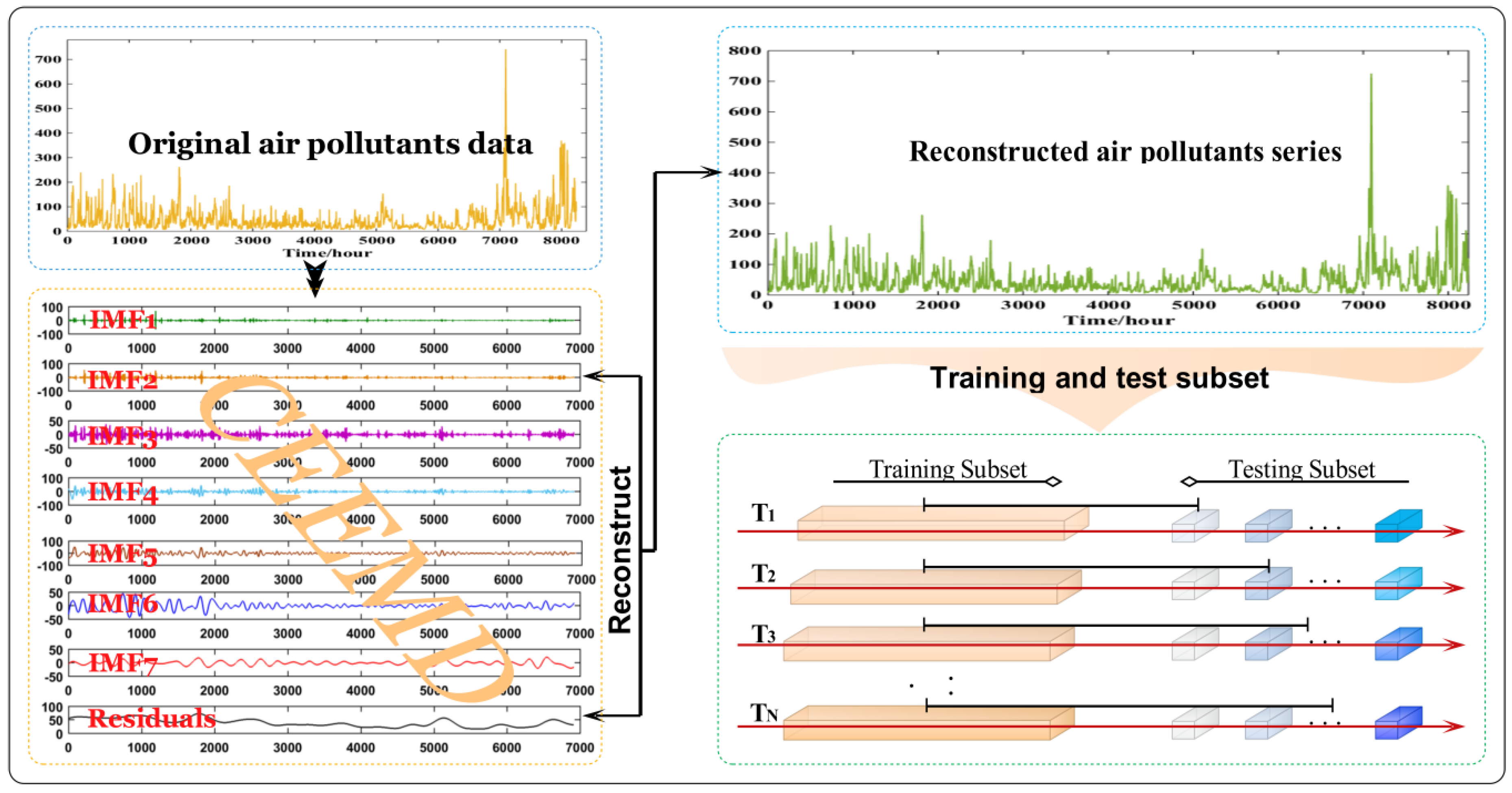
2.2. CEEMD
- (1)
- Given that a single white noise has no enough capability to solve all intermittent signals, we established a positive mixture f1(t) and a negative mixture f2(t) via appending a pair of white noise () to the original signal:
- (2)
- Afterward, kij+ and kij− are two ensembles of IMFs acquired from decomposing the positive and negative mixtures by the EMD, and kij+ or kij− is the jth IMF acquired via additive of the ith positive noise or negative noise.
- (3)
- Then, the final IMF is computed by:
- (4)
- (Accordingly, the original signal f(t) can be indicated via:where rn(t) is the n-th residue (i.e., local trend).
2.3. The Modified BBO Algorithm
2.4. LSSVM
2.5. Interval Forecasting Based on LSSVM
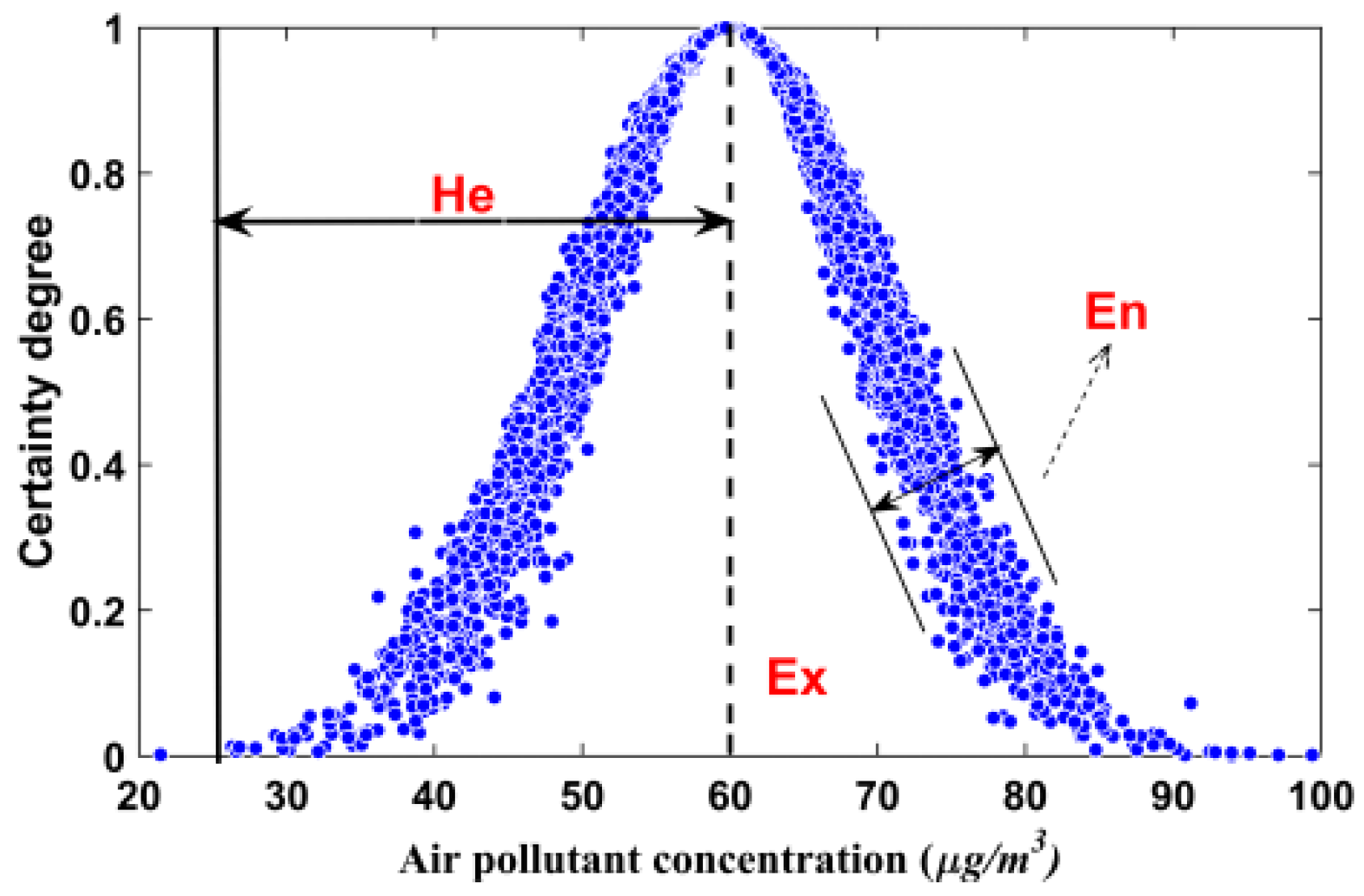
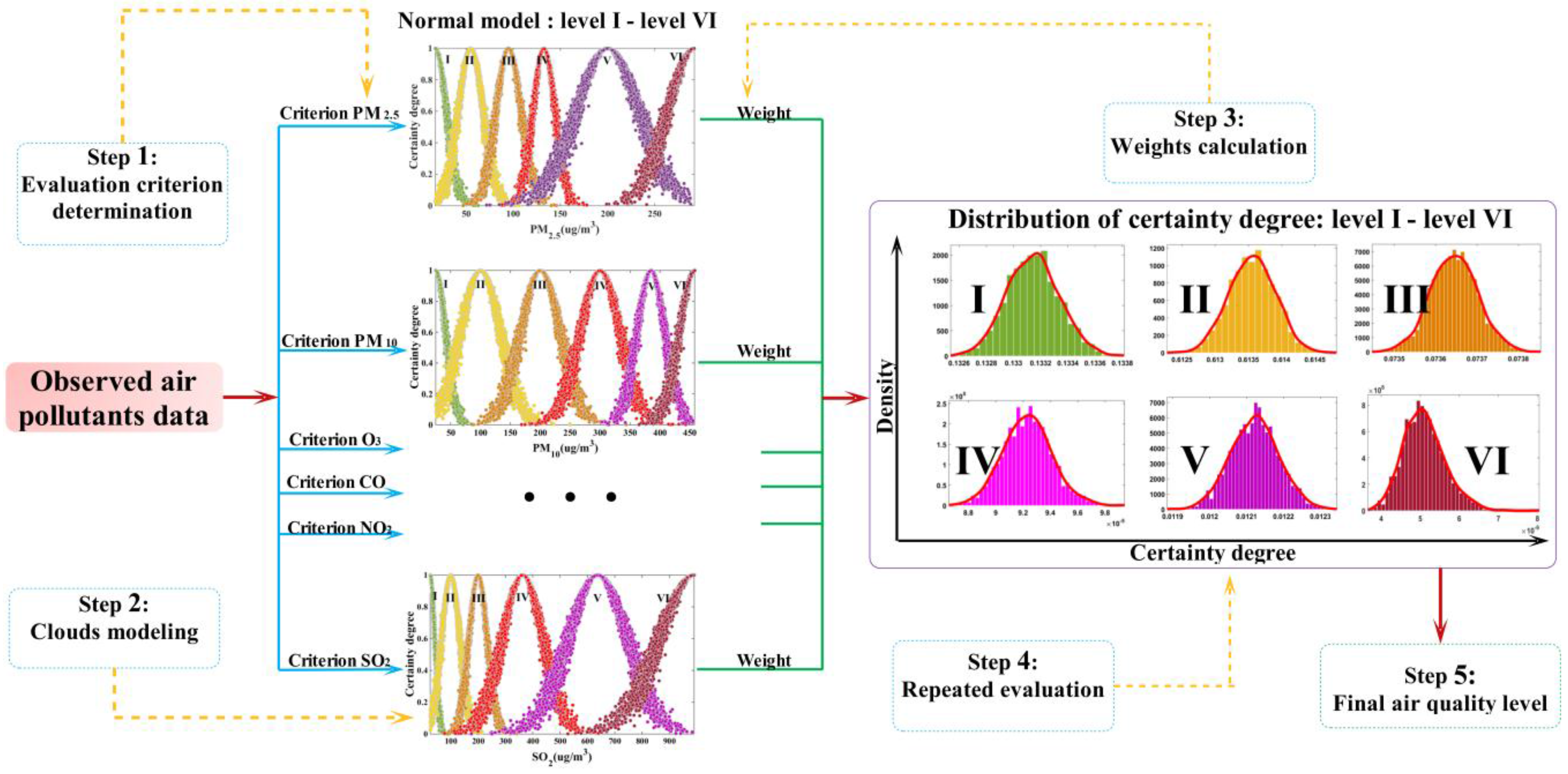
2.6. Normal Cloud Model Applied for Air Quality Evaluation
3. Simulation Modeling and Analysis
3.1. Modeling Preparations
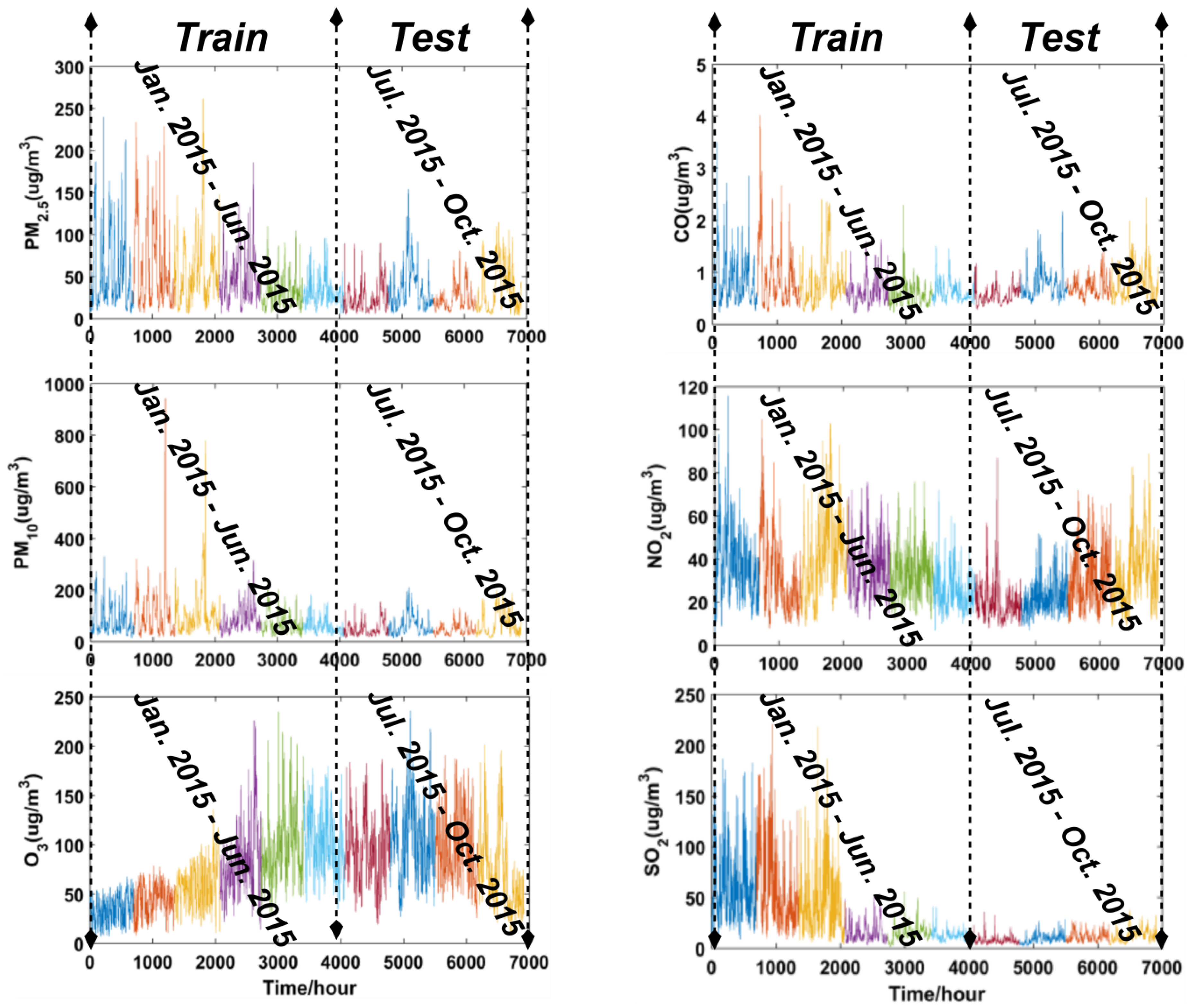
3.1.1. Study Site and Data Source
3.1.2. The Fitness Function for the CEEMD-BBODE-LSSVM Model
3.1.3. The Performance Metric
3.1.4. D-M Test
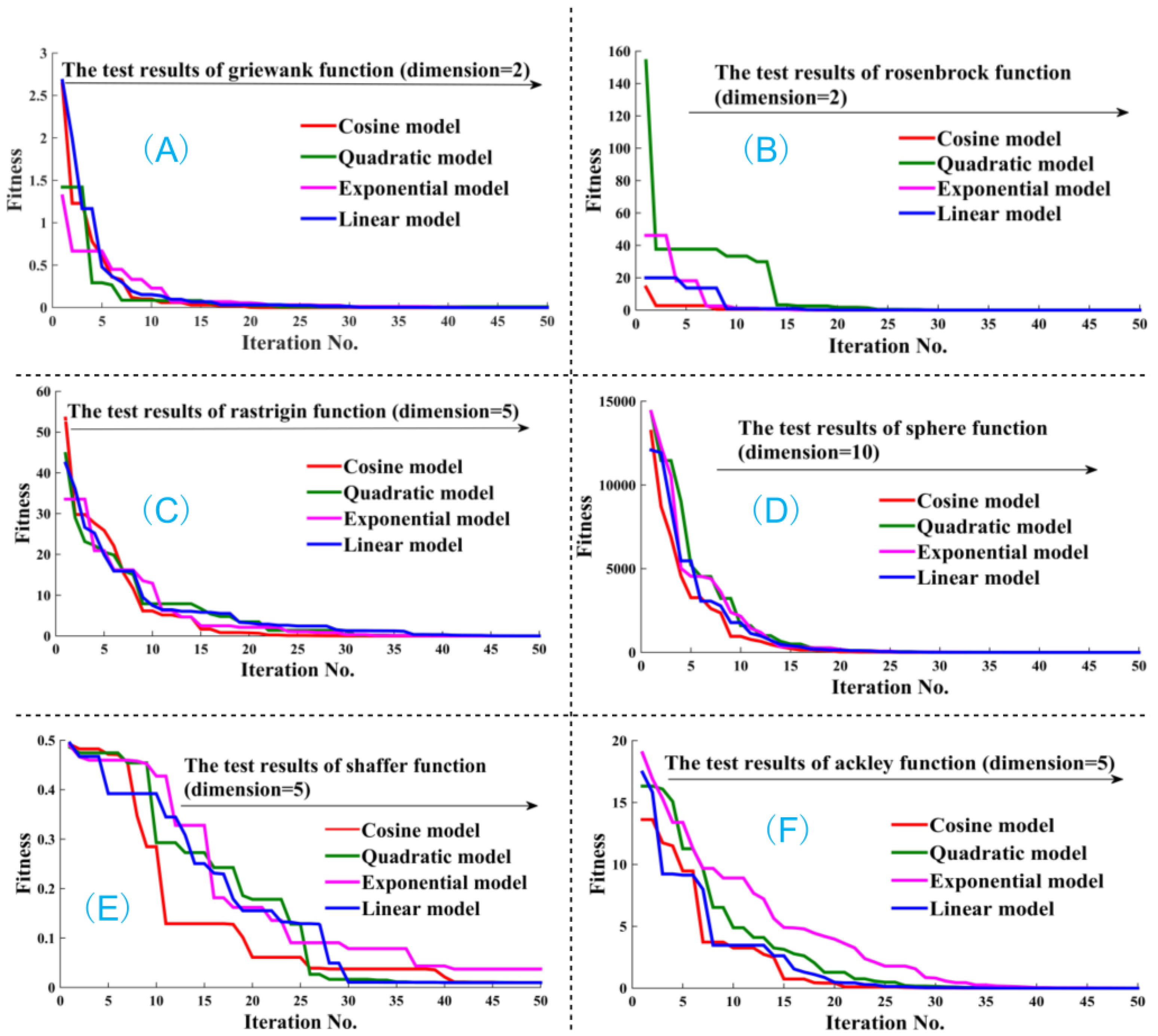
3.2. Numerical Analysis of the BBO and BBODE Algorithms
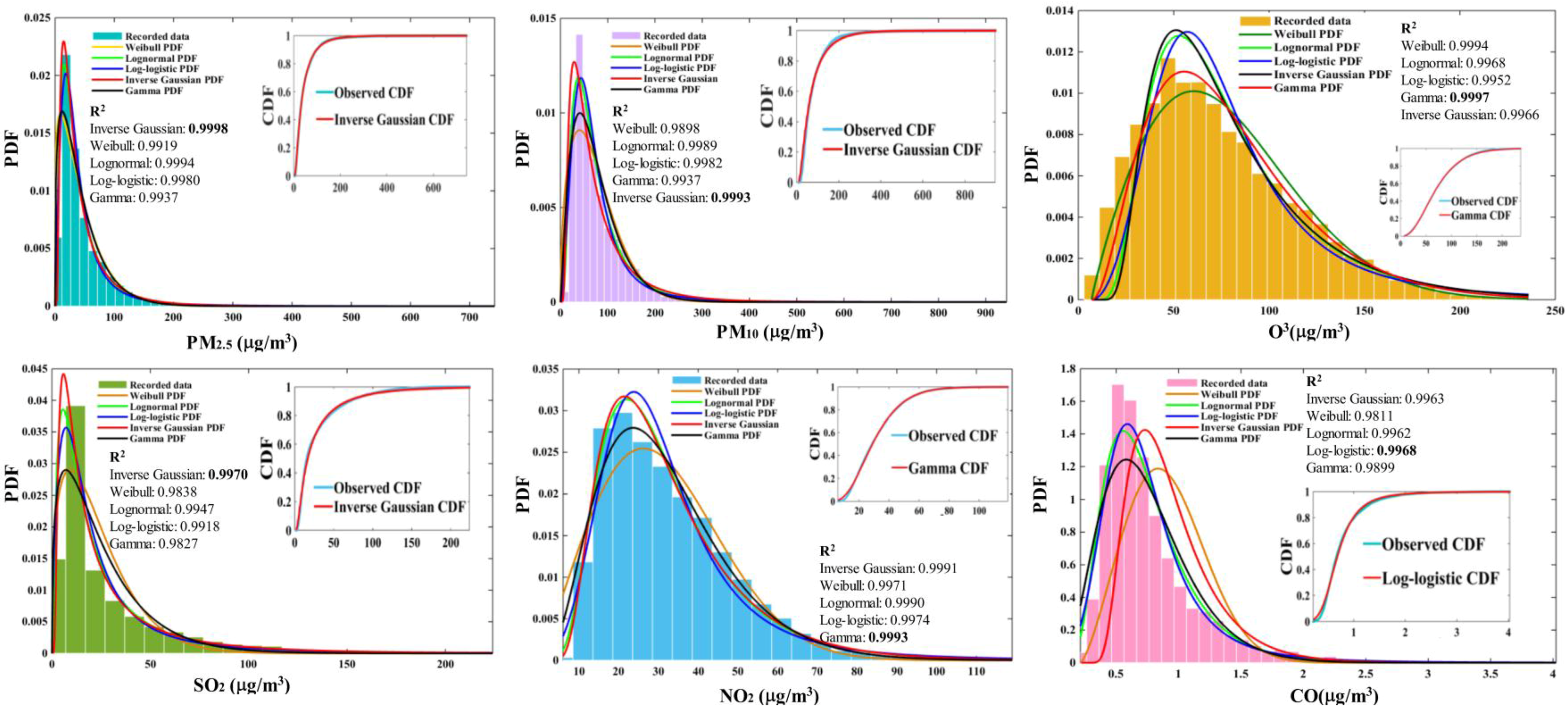
3.3. The Distributional Characteristics of the Air Pollutants
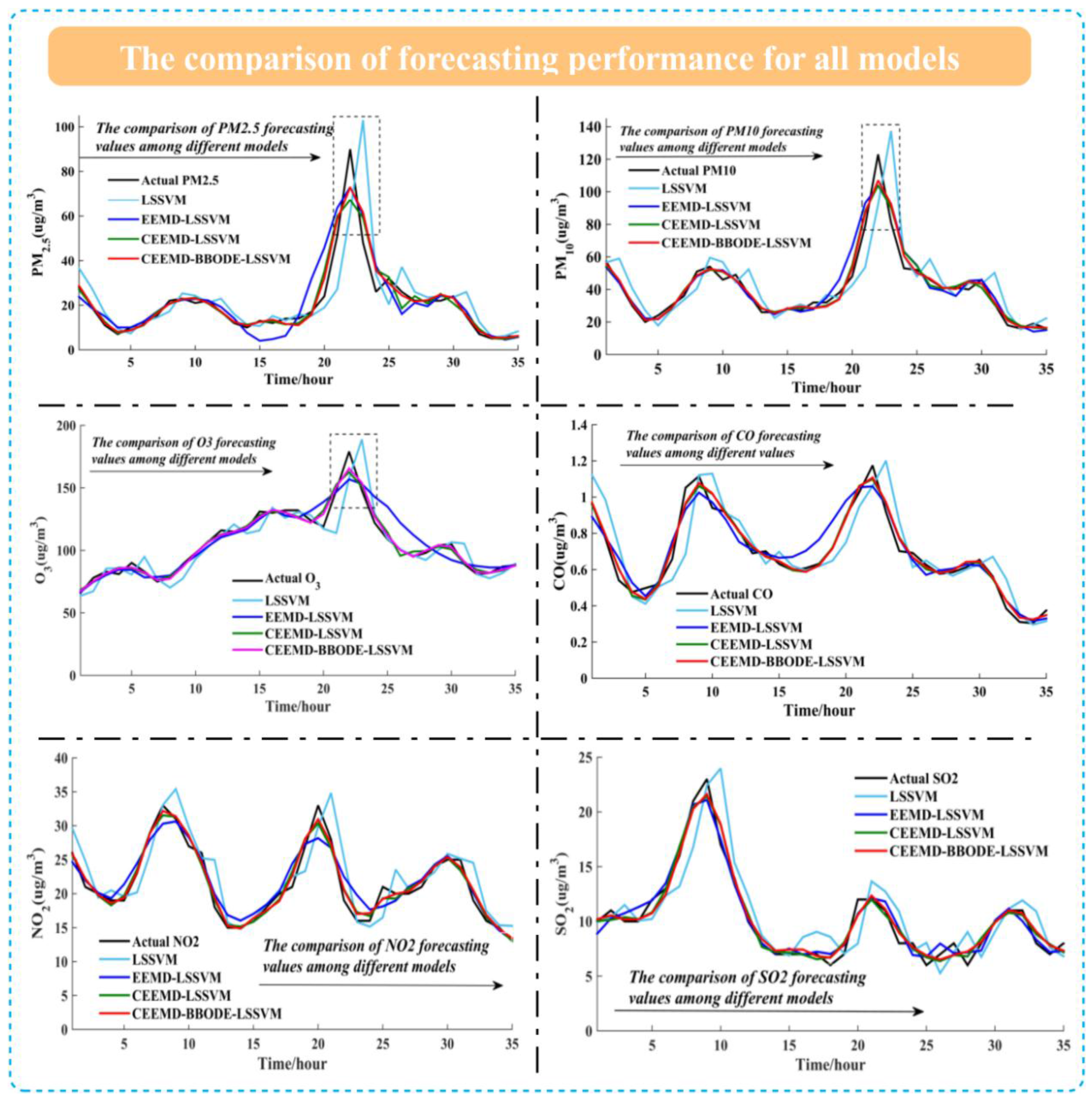
3.4. The Point Forecasting for Air Pollutants
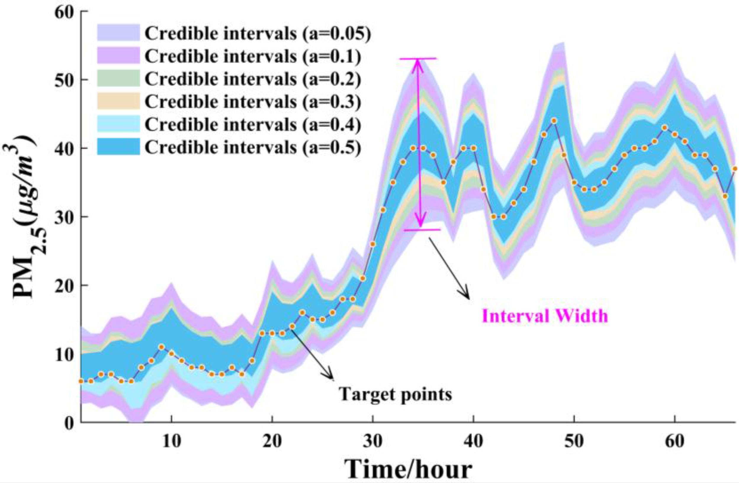
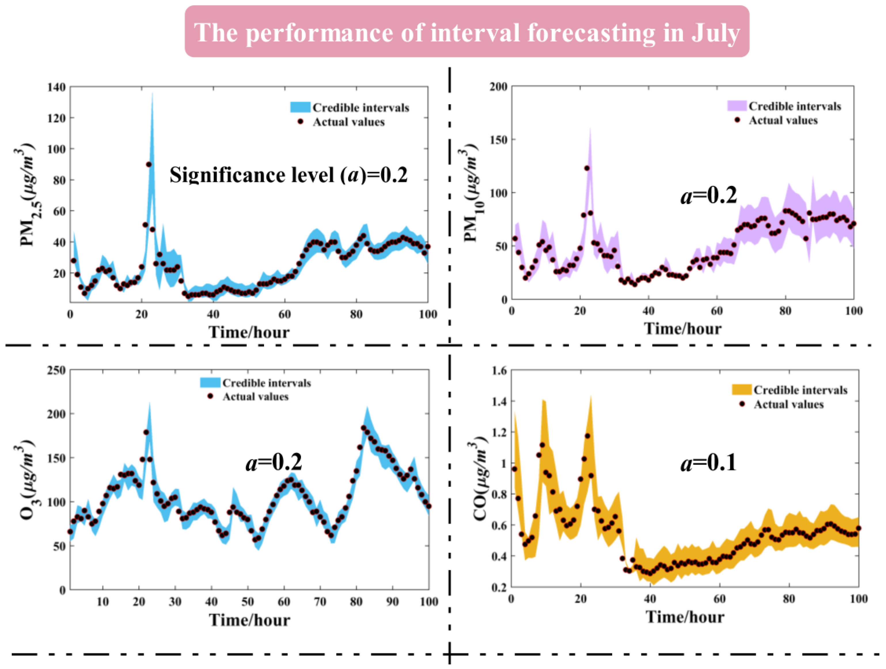
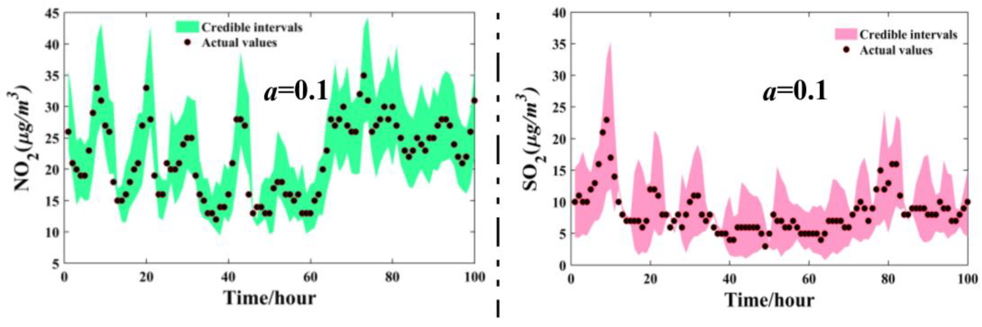
3.5. The Interval Forecasting for Air Pollutants
3.6. Comprehensive Evaluation Implementation
3.6.1. Evaluation Preparation
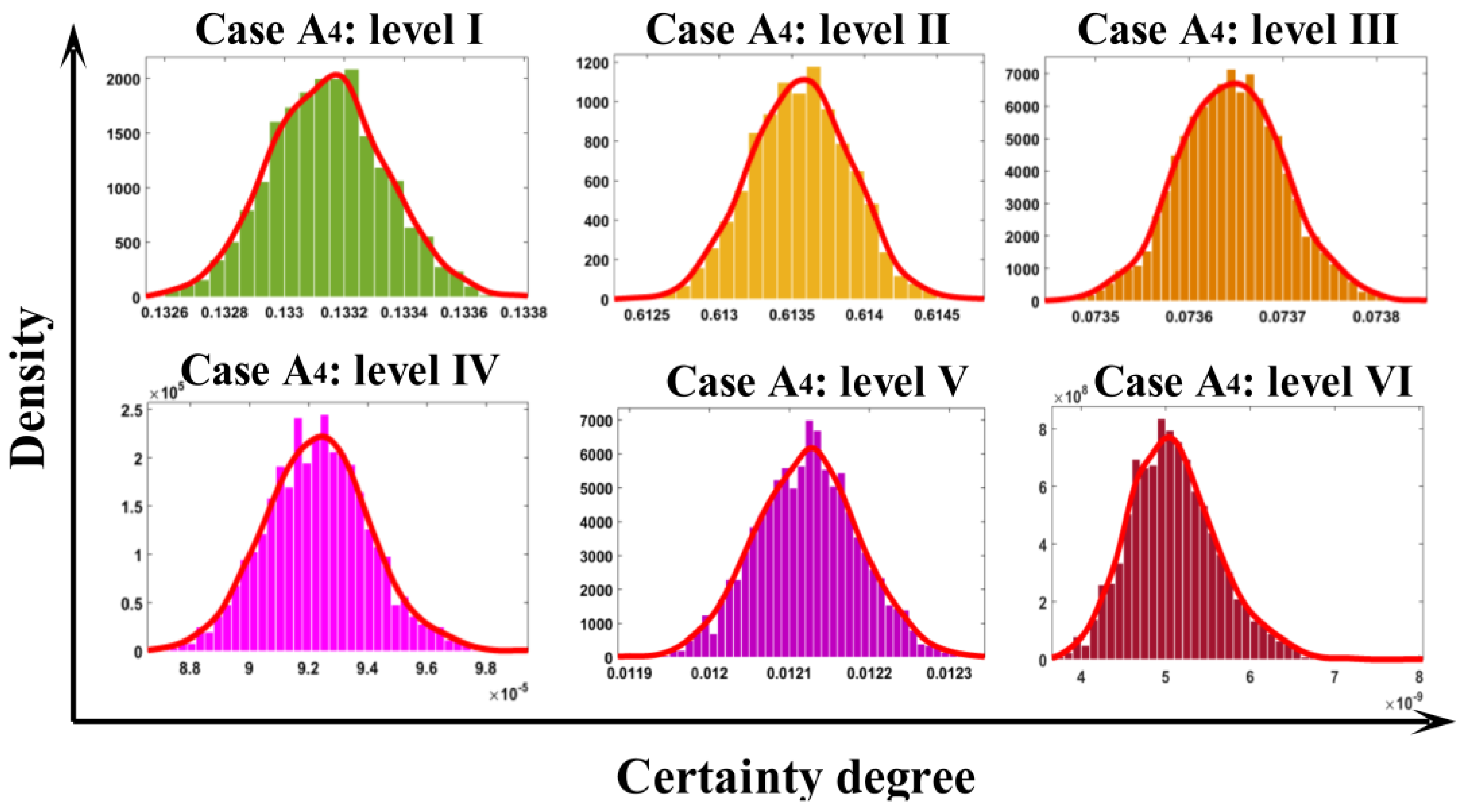
3.6.2. Evaluation Implementation
4. Discussion
4.1. The Forecasting Effectiveness Based on D-M Test
4.2. The Public Health Implications of the EWS
4.3. Future Considerations for the Air Quality EWS
5. Conclusions
Acknowledgments
Author Contributions
Conflicts of Interest
Abbreviations
| CTM | chemical transport model |
| MLR | multiple linear regression |
| ARIMA | integrated moving average model |
| GRNN | general regression neural network |
| LSSVM | least squares support vector machine |
| SVM | support vector machine |
| AHP | analytical hierarchical process |
| EMD | empirical mode decomposition |
| EEMD | ensemble empirical mode decomposition |
| CEEMD | complementary ensemble empirical mode decomposition |
| IMF | intrinsic mode function |
| DE | differential evolution |
| BBO | biogeography-based optimization |
| probabilistic distribution function | |
| CDF | cumulative distribution function |
| AW | average width |
| CP | coverage probability |
| AQI | air quality index |
| MAE | mean absolute error |
| MAPE | mean absolute percentage error |
| RMSE | root mean square error |
| R2 | goodness of fit |
| Std. | standard deviation |
Appendix A
Appendix 1. The PDF and CDF Functions for Weibull, Gamma, Lognormal, Log-Logistic, Inverse Gaussian

| Distribution | PDF/CDF | Parameters |
|---|---|---|
| Weibull | a > 0 scale parameter b > 0 shape parameter | |
| Gamma | a > 0 shape parameter b > 0 scale parameter | |
| Lognormal | a > 0 scale parameter b > 0 location parameter | |
| Log-logistic | a > 0 scale parameter b > 0 shape parameter | |
| Inverse Gaussian | a > 0 scale parameter b > 0 shape parameter | |
Appendix 2. The Test Functions in This Paper for BBO and BBODE Algorithm
| Function Name | Test Function | Variable Domain | Global Optimum |
|---|---|---|---|
| Sphere | |||
| Rosenbrock | |||
| Rastrigin | |||
| Shaffer | |||
| Griewank | |||
| Ackley |
Appendix 3. Pseudo-Code of the BBODE Algorithm
| Parameters |
| t: the number of iteration Iter_Max: the maximum number of iteration |
| n: the maximum number of species size: the size of population |
| rand: the random number in [0,1] Vi: the mixed hybrid operator |
| MaxXi: the maximum individual MinXi: the minimum individual |
| C: the probability of mutation F: difference operator |
| 1 /* Parameter setup */ |
| 2 /* Initialize population Pi */ |
| 3 /* Compute the fitness function Fi of each habitat, sort Fi */ |
| 4 |
| 5 /* Obtain elitist population */ |
| 6 /* Initialize probability of population in habitat */ |
| 7 FOR t < Iter_Max DO |
| 8 IF t is odd THEN |
| 9 /* Compute the number of population k */ |
| 10 /* Compute the rate of immigration λi and emigration μi for each habitat */ |
| 11 ; |
| 12 /* Normalize the immigration rate λscale */ |
| 13 |
| 14 /* Operation of migration */ |
| 15 Transform new information to habitat i |
| 16 ELSE |
| 17 FOR i = 1:size |
| 18 Choose indexes r1 ≠ r2 ≠ i |
| 19 /* Generate difference operator */ |
| 20 |
| 21 IF rand ≤ C THEN |
| 22 /* Mutation operation */ |
| 23 |
| 24 END IF |
| 25 END FOR |
| 26 END IF |
| 27 END FOR |
| 28 /* Deassign for samples beyond the range */ |
| 29 /* Deassign for the same sample */ |
| 30 /* Compute fitness Fi for new population and sort Fi */ |
| 31 Obtain optimal solution |
| 32 Postprocess results and visualization |
References
- Du, X.; Kong, Q.; Ge, W.; Zhang, S.; Fu, L. Characterization of personal exposure concentration of fine particles for adults and children exposed to high ambient concentrations in Beijing, China. J. Environ. Sci. China 2010, 22, 1757–1764. [Google Scholar] [CrossRef]
- Qiu, H.; Yu, I.T.S.; Wang, X.; Tian, L.; Tse, L.A.; Wong, T.W. Differential effects of fine and coarse particles on daily emergency cardiovascular hospitalizations in Hong Kong. Atmos. Environ. 2013, 64, 296–302. [Google Scholar] [CrossRef]
- MECC (Ministry of the Environment and Climate Change). Fine Particulate Matter 2012; Ministry of the Environment and Climate Change: Scarborough, ON, Canada, 2012.
- Cobourn, W.G. An enhanced PM2.5, air quality forecast model based on nonlinear regression and back-trajectory concentrations. Atmos. Environ. 2010, 44, 3015–3023. [Google Scholar] [CrossRef]
- Sun, W.; Zhang, H.; Palazoglu, A.; Singh, A.; Zhang, W.; Liu, S. Prediction of 24-hour-average PM2.5, concentrations using a hidden Markov model with different emission distributions in Northern California. Sci. Total Environ. 2013, 443, 93–103. [Google Scholar] [CrossRef] [PubMed]
- Han, Z.; Ueda, H.; An, J. Evaluation and intercomparison of meteorological predictions by five MM5-PBL parameterizations in combination with three land-surface models. Atmos. Environ. 2008, 42, 233–249. [Google Scholar] [CrossRef]
- Konovalov, I.B.; Beekmann, M.; Meleux, F.; Dutot, A.; Foret, G. Combining deterministic and statistical approaches for PM10, forecasting in Europe. Atmos. Environ. 2009, 43, 6425–6434. [Google Scholar] [CrossRef]
- Wongsathan, R.; Seedadan, I. A Hybrid ARIMA and Neural Networks Model for PM-10 Pollution Estimation: The Case of Chiang Mai City Moat Area. Procedia Comput. Sci. 2016, 86, 273–276. [Google Scholar] [CrossRef]
- Song, Y.; Qin, S.; Qu, J.; Liu, F. The forecasting research of early warning systems for atmospheric pollutants: A case in Yangtze River Delta region. Atmos. Environ. 2015, 118, 58–69. [Google Scholar] [CrossRef]
- Prasad, K.; Gorai, A.K.; Goyal, P. Development of ANFIS models for air quality forecasting and input optimization for reducing the computational cost and time. Atmos. Environ. 2016, 128, 246–262. [Google Scholar] [CrossRef]
- Qin, S.; Liu, F.; Wang, J.; Sun, B. Analysis and forecasting of the particulate matter (PM) concentration levels over four major cities of China using hybrid models. Atmos. Environ. 2014, 98, 665–675. [Google Scholar] [CrossRef]
- Niu, M.; Wang, Y.; Sun, S.; Li, Y. A novel hybrid decomposition-and-ensemble model based on CEEMD and GWO for short-term PM concentration forecasting. Atmos. Environ. 2016, 134, 168–180. [Google Scholar] [CrossRef]
- Zhou, Q.; Jiang, H.; Wang, J.; Zhou, J. A hybrid model for PM2.5, forecasting based on ensemble empirical mode decomposition and a general regression neural network. Sci. Total Environ. 2014, 496C, 264–274. [Google Scholar] [CrossRef] [PubMed]
- Gorai, A.K.; Upadhyay, A.; Tuluri, F.; Goyal, P.; Tchounwou, P.B. An innovative approach for determination of air quality health index. Sci. Total Environ. 2015, 533, 495–505. [Google Scholar] [CrossRef] [PubMed]
- Zhao, X.; Qi, Q.; Li, R. The establishment and application of fuzzy comprehensive model with weight based on entropy technology for air quality assessment. Procedia Eng. 2010, 7, 217–222. [Google Scholar] [CrossRef]
- Olvera-García, M.Á.; Carbajal-Hernández, J.J.; Sánchez-Fernández, L.P.; Hernández-Bautista, I. Air quality assessment using a weighted Fuzzy Inference System. Ecol. Inform. 2016, 33, 57–74. [Google Scholar] [CrossRef]
- Huang, N.E.; Shen, Z.; Long, S.R.; Wu, M.C.; Shih, H.H.; Zheng, Q.; Yen, N.C.; Tung, C.C.; Liu, H.H. The Empirical Mode Decomposition and the Hilbert Spectrum for Nonlinear and Non-stationary Time Series Analysis. Proc. R. Soc. A Math. Phys. Eng. Sci. 1998, 454, 903–995. [Google Scholar] [CrossRef]
- Huang, N.E.; Wu, M.L.C.; Long, S.R.; Shen, S.S.; Qu, W.; Gloersen, P.; Fan, K.L. A confidence limit for the empirical mode decomposition and Hilbert spectral analysis. Proc. R. Soc. A 2003, 459, 2317–2345. [Google Scholar] [CrossRef]
- Oberlin, T.; Meignen, S.; Perrier, V. An Alternative Formulation for the Empirical Mode Decomposition. IEEE Trans. Signal Process. 2012, 60, 2236–2246. [Google Scholar] [CrossRef]
- Chen, Q.; Huang, N.; Riemenschneider, S.; Xu, Y. A B-spline approach for empirical mode decompositions. Adv. Comput. Math. 2006, 24, 171–195. [Google Scholar] [CrossRef]
- Sharpley, R.C.; Vatchev, V. Analysis of the Intrinsic Mode Functions. Constr. Approx. 2006, 24, 17–47. [Google Scholar] [CrossRef]
- Peng, Z.K.; Tse, P.W.; Chu, F.L. A comparison study of improved Hilbert–Huang transform and wavelet transform: Application to fault diagnosis for rolling bearing. Mech. Syst. Signal Process. 2005, 19, 974–988. [Google Scholar] [CrossRef]
- Yeh, J.; Shieh, J.; Norden, E.; Huang, N.E. Complementary ensemble empirical mode decomposition: A novel noise enhanced data analysis method. Adv. Adapt. Data Anal. 2010, 2, 135–156. [Google Scholar] [CrossRef]
- Imaouchen, Y.; Kedadouche, M.; Alkama, R.; Thomas, M. A Frequency-Weighted Energy Operator and complementary ensemble empirical mode decomposition for bearing fault detection. Mech. Syst. Signal Process. 2016, 82, 103–116. [Google Scholar] [CrossRef]
- Simon, D. Biogeography-Based Optimization. IEEE Trans. Evolut. Comput. 2008, 12, 702–713. [Google Scholar] [CrossRef]
- Rarick, R.; Simon, D.; Villaseca, F.E.; Vyakaranam, B. Biogeography-based optimization and the solution of the power flow problem. In Proceedings of the IEEE International Conference on Systems, Man and Cybernetics, San Antonio, TX, USA, 11–14 October 2009; pp. 1003–1008.
- Roy, P.K.; Ghoshal, S.P.; Thakur, S.S. Biogeography-based Optimization for Economic Load Dispatch Problems. Electr. Power Compon. Syst. 2010, 38, 166–181. [Google Scholar] [CrossRef]
- Kundra, H.; Kaur, A.; Panchal, V. An integrated approach to biogeography based optimization with case based reasoning for retrieving groundwater possibility. In Proceedings of the 8th Annual Asian Conference and Exhibition on Geospatial Information, Technology and Applications, Singapore, 18–20 August 2009.
- Panchal, V.K.; Singh, P.; Kaur, N.; Kundra, H. Biogeography based Satellite Image Classification. Comput. Sci. 2009, 6, 269–274. [Google Scholar]
- Vapnik, V.N. The Nature of Statistical Learning Theory; Springer: Berlin, Germany, 2000; pp. 988–999. [Google Scholar]
- Suykens, J.A.K.; Vandewalle, J. Least Squares Support Vector Machine Classifiers. Neural Process. Lett. 1999, 9, 293–300. [Google Scholar] [CrossRef]
- Wang, J.; Hu, J. A robust combination approach for short-term wind speed forecasting and analysis—Combination of the ARIMA, ELM, SVM and LSSVM forecasts using a GPR model. Energy 2015, 93, 41–56. [Google Scholar] [CrossRef]
- Keerthi, S.S.; Lin, C.J. Asymptotic behaviors of support vector machines with gaussian kernel. Neural Comput. 2003, 15, 1667–1689. [Google Scholar] [CrossRef] [PubMed]
- De Brabanter, K.; De Brabanter, J.; Suykens, J.A.; De Moor, B. Approximate Confidence and Prediction Intervals for Least Squares Support Vector Regression. IEEE Trans. Neural Netw. 2011, 22, 110–120. [Google Scholar] [CrossRef] [PubMed]
- Li, D.; Liu, C.; Gan, W. A new cognitive model: Cloud model. Int. J. Intell. Syst. 2009, 24, 357–375. [Google Scholar] [CrossRef]
- Wang, D.; Liu, D.; Ding, H.; Singh, V.P.; Wang, Y.; Zeng, X.; Wu, J.; Wang, L. A cloud model-based approach for water quality assessment. Environ. Res. 2016, 148, 24–35. [Google Scholar] [CrossRef] [PubMed]
- Zhang, J.G.; Singh, V.P. Entropy-Theory and Application; China Water & Power Press: Beijing, China, 2012; pp. 79–80. [Google Scholar]
- Diebold, F.X.; Mariano, R.S. Comparing Predictive Accuracy. NBER Tech. Work. Pap. 1994, 13, 134–144. [Google Scholar]
- Xiao, L.; Wang, J.; Hou, R.; Wu, J. A combined model based on data pre-analysis and weight coefficients optimization for electrical load forecasting. Energy 2015, 82, 524–549. [Google Scholar] [CrossRef]


| Levels | Air Quality Criteria (µg/m3) | |||||
|---|---|---|---|---|---|---|
| PM2.5 | PM10 | O3 | CO | NO2 | SO2 | |
| I | ≤35 | ≤50 | ≤10 | ≤2 | ≤40 | ≤50 |
| II | ≤75 | ≤150 | ≤160 | ≤4 | ≤80 | ≤150 |
| III | ≤115 | ≤250 | ≤215 | ≤14 | ≤180 | ≤250 |
| IV | ≤150 | ≤350 | ≤265 | ≤24 | ≤280 | ≤475 |
| V | ≤250 | ≤420 | ≤800 | ≤36 | ≤565 | ≤800 |
| VI | >250 | >420 | >800 | >36 | >565 | >800 |
| Metric | Definition | Equation |
|---|---|---|
| MAE | Mean absolute error | |
| MAPE | Mean absolute percentage error | |
| RMSE | Root mean square error | |
| R2 | Goodness of fit |
| Parameter Setting | BBO | BBODE |
|---|---|---|
| Maximum iteration | 5000 | 5000 |
| Population size | 50 | 50 |
| The number of elite kept | 3 | 3 |
| Maximum emigration rate | 1 | 1 |
| Minimum emigration rate | 0 | 0 |
| Maximum immigration rate | 1 | 1 |
| Minimum immigration rate | 0 | 0 |
| Mutation probability | 0.05 | 0.4 |
| Difference operator | - | 0.6 |
| Test Function | Dimension | Algorithm | Optimal/Worse Solution | Mean/Std. | Elapsed Time (s) |
|---|---|---|---|---|---|
| Sphere | 5 | BBO | 3.83 × 10⁻³/1.87 × 10−2 | 1.21 × 10⁻²/6.09 × 10−3 | 24.5293 |
| BBODE | 0/0 | 0/0 | 25.1026 | ||
| 10 | BBO | 1.05 × 10⁻²/3.42 × 10−1 | 8.06 × 10⁻²/3.14 × 10−2 | 27.1782 | |
| BBODE | 0/0 | 0/0 | 28.0055 | ||
| Rosenbrock | 2 | BBO | 1.05 × 10⁻²/6.19 × 10−1 | 2.65 × 10⁻¹/2.48 × 10−1 | 21.5151 |
| BBODE | 0/0 | 0/0 | 38.8187 | ||
| Rastrigin | 2 | BBO | 1.56 × 10⁻⁴/3.71 × 10−3 | 1.70 × 10⁻³/1.46 × 10−3 | 22.1951 |
| BBODE | 0/0 | 0/0 | 23.0743 | ||
| 5 | BBO | 3.97 × 10⁻³/2.05 × 10−2 | 1.15 × 10⁻²/6.43 × 10−3 | 24.4002 | |
| BBODE | 0/0 | 0/0 | 24.1739 | ||
| Shaffer | 2 | BBO | 9.72 × 10⁻³/3.33 × 10−2 | 1.45 × 10⁻²/1.06 × 10−2 | 22.4175 |
| BBODE | 0/0 | 0/0 | 23.3923 | ||
| 5 | BBO | 9.72 × 10⁻³/7.82 × 10−2 | 3.99 × 10⁻²/2.45 × 10−2 | 24.3080 | |
| BBODE | 9.72 × 10⁻³/9.72 × 10−3 | 9.70 × 10⁻³/9.23 × 10−11 | 29.3161 | ||
| Griewank | 2 | BBO | 3.60 × 10⁻³/6.80 × 10−2 | 2.06 × 10⁻²/2.67 × 10−2 | 22.2211 |
| BBODE | 0/7.40 × 10−3 | 3.00 × 10⁻³/4.05 ×10−3 | 22.4311 | ||
| Ackley | 2 | BBO | 2.61 × 10⁻²/8.12 × 10−2 | 5.24 × 10⁻²/2.57 × 10−2 | 22.4061 |
| BBODE | 8.88 × 10⁻¹⁶/8.88 × 10−16 | 0/0 | 22.9809 | ||
| 5 | BBO | 2.78 × 10⁻²/2.90 × 10−1 | 1.20 × 10⁻¹/1.07 × 10−1 | 24.3998 | |
| BBODE | 8.88 × 10⁻¹⁶/8.88 × 10−16 | 0/0 | 25.2199 |
| Indexes | Optimized Algorithm | Parameters | |||||||||
|---|---|---|---|---|---|---|---|---|---|---|---|
| Weibull | Gamma | Lognormal | Log-Logistic | Inverse Gaussian | |||||||
| a | b | a | b | a | b | a | b | a | b | ||
| PM2.5 | BBO | 45.6353 | 1.1494 | 1.1219 | 39.3960 | 0.9590 | 3.3423 | 1.9971 | 31.9631 | 46.2247 | 47.6059 |
| BBODE | 45.7883 | 1.1754 | 1.3769 | 31.5937 | 0.8675 | 3.4642 | 1.9865 | 32.0344 | 46.1661 | 47.6248 | |
| PM10 | BBO | 82.0580 | 1.3799 | 4.5728 | 15.1932 | 0.7351 | 3.9522 | 2.6477 | 62.4040 | 77.6225 | 137.8372 |
| BBODE | 82.1414 | 1.5152 | 2.2187 | 33.7894 | 0.6939 | 4.1205 | 2.4676 | 61.5932 | 78.0797 | 137.2609 | |
| O3 | BBO | 81.9614 | 1.8979 | 3.7011 | 19.7425 | 0.6156 | 4.0754 | 3.0971 | 65.1357 | 76.2749 | 199.8628 |
| BBODE | 82.0189 | 1.8920 | 3.0735 | 24.0945 | 0.5648 | 4.1715 | 3.0136 | 64.9673 | 75.8027 | 213.8432 | |
| SO2 | BBO | 27.1355 | 1.1097 | 0.9696 | 28.5482 | 2.8314 | 1.0833 | 1.6724 | 17.3678 | 27.1713 | 19.4500 |
| BBODE | 26.4620 | 0.9312 | 0.9194 | 29.4822 | 2.8378 | 1.0554 | 1.6357 | 17.1035 | 29.3444 | 18.3036 | |
| NO2 | BBO | 35.1287 | 2.1449 | 3.8436 | 8.2904 | 0.5596 | 3.2623 | 3.2489 | 28.1741 | 32.5209 | 112.2516 |
| BBODE | 35.2476 | 2.1360 | 3.8948 | 8.1566 | 0.5075 | 3.3501 | 3.3673 | 28.5397 | 32.3743 | 114.6579 | |
| CO | BBO | 0.8547 | 2.2424 | 1.1233 | 0.7854 | 0.4562 | −0.3797 | 3.8337 | 0.7208 | 1.0952 | 1.0957 |
| BBODE | 0.8229 | 2.3983 | 4.4389 | 0.1689 | 0.4558 | −0.3789 | 3.7101 | 0.6832 | 0.7589 | 3.3818 | |
| Indexes | Optimized Algorithm | Evaluation Criteria (R2) | ||||
|---|---|---|---|---|---|---|
| Weibull | Gamma | Lognormal | Log-Logistic | Inverse Gaussian | ||
| PM2.5 | BBO | 0.9918 | 0.9904 | 0.9919 | 0.9980 | 0.9998 |
| BBODE | 0.9919 | 0.9937 | 0.9994 | 0.9980 | 0.9998 | |
| PM10 | BBO | 0.9879 | 0.9634 | 0.9760 | 0.9970 | 0.9991 |
| BBODE | 0.9898 | 0.9937 | 0.9989 | 0.9982 | 0.9993 | |
| O3 | BBO | 0.9984 | 0.9979 | 0.9870 | 0.9950 | 0.9963 |
| BBODE | 0.9994 | 0.9997 | 0.9968 | 0.9952 | 0.9966 | |
| SO2 | BBO | 0.9747 | 0.9820 | 0.9944 | 0.9916 | 0.9942 |
| BBODE | 0.9838 | 0.9827 | 0.9947 | 0.9918 | 0.9970 | |
| NO2 | BBO | 0.9971 | 0.9990 | 0.9901 | 0.9970 | 0.9991 |
| BBODE | 0.9971 | 0.9993 | 0.9990 | 0.9974 | 0.9991 | |
| CO | BBO | 0.9774 | 0.8257 | 0.9962 | 0.9894 | 0.8309 |
| BBODE | 0.9811 | 0.9899 | 0.9962 | 0.9968 | 0.9963 | |
| Jul. | LSSVM | EEMD-LSSVM | CEEMD-LSSVM | CEEMD-BBODE-LSSVM | ||||||||||||
| MAE (µg/m3) | MAPE (%) | RMSE (µg/m3) | R2 | MAE (µg/m3) | MAPE (%) | RMSE (µg/m3) | R2 | MAE (µg/m3) | MAPE (%) | RMSE (µg/m3) | R2 | MAE (µg/m3) | MAPE (%) | RMSE (µg/m3) | R2 | |
| PM2.5 | 2.7493 | 13.72 | 4.6403 | 0.9190 | 1.5257 | 7.01 | 2.8392 | 0.9697 | 0.9223 | 4.24 | 1.7455 | 0.9885 | 0.8377 | 3.86 | 1.5264 | 0.9912 |
| PM10 | 4.7844 | 10.87 | 7.6946 | 0.9228 | 2.3329 | 5.17 | 3.7108 | 0.9821 | 1.5476 | 3.46 | 2.5508 | 0.9915 | 1.5004 | 3.34 | 2.4581 | 0.9921 |
| O3 | 5.7668 | 6.81 | 7.9288 | 0.9451 | 3.0425 | 3.56 | 4.4377 | 0.9828 | 1.9619 | 2.27 | 2.7241 | 0.9935 | 1.7602 | 2.04 | 2.4161 | 0.9949 |
| CO | 0.0282 | 4.93 | 0.0461 | 0.9021 | 0.0137 | 2.39 | 0.0225 | 0.9766 | 0.0094 | 1.64 | 0.0153 | 0.9892 | 0.0093 | 1.64 | 0.0150 | 0.9896 |
| NO2 | 2.4432 | 12.82 | 3.6164 | 0.8298 | 1.2705 | 6.61 | 1.8767 | 0.9542 | 0.8877 | 4.65 | 1.3733 | 0.9755 | 0.8138 | 4.29 | 1.2850 | 0.9785 |
| SO2 | 1.3173 | 17.17 | 1.9538 | 0.7346 | 0.6607 | 8.92 | 0.9071 | 0.9428 | 0.5091 | 6.71 | 0.7596 | 0.9599 | 0.4762 | 6.42 | 0.7222 | 0.9637 |
| Aug. | LSSVM | EEMD-LSSVM | CEEMD-LSSVM | CEEMD-BBODE-LSSVM | ||||||||||||
| MAE (µg/m3) | MAPE (%) | RMSE (µg/m3) | R2 | MAE (µg/m3) | MAPE (%) | RMSE (µg/m3) | R2 | MAE (µg/m3) | MAPE (%) | RMSE (µg/m3) | R2 | MAE (µg/m3) | MAPE (%) | RMSE (µg/m3) | R2 | |
| PM2.5 | 2.8102 | 10.12 | 4.2173 | 0.9718 | 1.3468 | 4.72 | 2.0854 | 0.9931 | 0.9601 | 3.35 | 1.4169 | 0.9968 | 0.8584 | 3.00 | 1.2814 | 0.9974 |
| PM10 | 4.6826 | 8.27 | 7.9020 | 0.9517 | 4.6866 | 8.32 | 7.8981 | 0.9518 | 1.4682 | 2.55 | 2.4766 | 0.9953 | 1.4201 | 2.47 | 2.4687 | 0.9953 |
| O3 | 6.8965 | 7.19 | 9.2676 | 0.9454 | 4.3948 | 4.66 | 5.7059 | 0.9793 | 2.1932 | 2.30 | 2.9572 | 0.9944 | 1.9939 | 2.05 | 2.6971 | 0.9954 |
| CO | 0.0382 | 4.83 | 0.0628 | 0.9453 | 0.0196 | 2.52 | 0.0350 | 0.9830 | 0.0126 | 1.65 | 0.0196 | 0.9946 | 0.0123 | 1.63 | 0.0192 | 0.9949 |
| NO2 | 2.6935 | 12.67 | 3.8906 | 0.7507 | 1.7882 | 8.44 | 2.5133 | 0.8960 | 1.1073 | 5.11 | 1.5708 | 0.9594 | 0.9906 | 4.62 | 1.4239 | 0.9666 |
| SO2 | 1.4433 | 16.43 | 2.0774 | 0.7876 | 0.7174 | 8.49 | 0.9874 | 0.9520 | 0.5274 | 6.17 | 0.7691 | 0.9709 | 0.5124 | 6.05 | 0.7568 | 0.9718 |
| Sept. | LSSVM | EEMD-LSSVM | CEEMD-LSSVM | CEEMD-BBODE-LSSVM | ||||||||||||
| MAE (µg/m3) | MAPE (%) | RMSE (µg/m3) | R2 | MAE (µg/m3) | MAPE (%) | RMSE (µg/m3) | R2 | MAE (µg/m3) | MAPE (%) | RMSE (µg/m3) | R2 | MAE (µg/m3) | MAPE (%) | RMSE (µg/m3) | R2 | |
| PM2.5 | 1.8597 | 9.26 | 2.6744 | 0.9632 | 0.8473 | 3.91 | 1.2725 | 0.9917 | 0.5845 | 2.73 | 0.8504 | 0.9963 | 0.5329 | 2.55 | 0.7836 | 0.9968 |
| PM10 | 3.1881 | 7.25 | 4.6004 | 0.9544 | 1.4800 | 3.29 | 2.0462 | 0.9910 | 0.9906 | 2.15 | 1.4081 | 0.9957 | 0.9464 | 2.10 | 1.3310 | 0.9962 |
| O3 | 6.1037 | 7.12 | 8.4823 | 0.9444 | 3.8598 | 4.52 | 5.5017 | 0.9766 | 1.9423 | 2.30 | 2.6734 | 0.9945 | 1.7936 | 2.10 | 2.4833 | 0.9952 |
| CO | 0.0343 | 4.80 | 0.0501 | 0.9231 | 0.0337 | 4.70 | 0.0501 | 0.9229 | 0.0108 | 1.51 | 0.0159 | 0.9922 | 0.0106 | 1.49 | 0.0155 | 0.9926 |
| NO2 | 3.3152 | 11.05 | 4.7473 | 0.8577 | 2.5733 | 9.40 | 3.6797 | 0.9145 | 1.3327 | 4.44 | 1.9169 | 0.9768 | 1.1959 | 3.99 | 1.7156 | 0.9814 |
| SO2 | 1.5666 | 14.18 | 2.1999 | 0.6901 | 6.46 | 0.9278 | 0.9611 | 0.5627 | 5.08 | 0.8056 | 0.9707 | 0.5429 | 4.87 | 0.7764 | 0.9728 | |
| Oct. | LSSVM | EEMD-LSSVM | CEEMD-LSSVM | CEEMD-BBODE-LSSVM | ||||||||||||
| MAE (µg/m3) | MAPE (%) | RMSE (µg/m3) | R2 | MAE (µg/m3) | MAPE (%) | RMSE (µg/m3) | R2 | MAE (µg/m3) | MAPE (%) | RMSE (µg/m3) | R2 | MAE (µg/m3) | MAPE (%) | RMSE (µg/m3) | R2 | |
| PM2.5 | 3.1429 | 14.75 | 5.2280 | 0.9632 | 2.0940 | 7.18 | 3.9670 | 0.9788 | 1.0080 | 4.02 | 1.8061 | 0.9956 | 0.9656 | 3.87 | 1.6485 | 0.9963 |
| PM10 | 5.5187 | 9.84 | 8.9370 | 0.9596 | 3.3163 | 5.39 | 5.7764 | 0.9831 | 1.7639 | 2.98 | 2.9540 | 0.9956 | 1.7107 | 2.64 | 2.8270 | 0.9960 |
| O3 | 5.2873 | 8.89 | 7.5633 | 0.9622 | 3.1799 | 5.05 | 4.6041 | 0.9860 | 1.7490 | 2.99 | 2.5731 | 0.9956 | 1.5749 | 2.70 | 2.3123 | 0.9965 |
| CO | 0.0491 | 6.26 | 0.0883 | 0.9185 | 0.0475 | 6.09 | 0.0846 | 0.9251 | 0.0173 | 2.22 | 0.0329 | 0.9887 | 0.0171 | 2.10 | 0.0318 | 0.9895 |
| NO2 | 3.2192 | 10.74 | 4.6240 | 0.9025 | 2.4256 | 8.04 | 3.7272 | 0.9366 | 1.2379 | 4.13 | 1.8160 | 0.9850 | 1.1440 | 3.81 | 1.6778 | 0.9872 |
| SO2 | 1.5912 | 14.01 | 2.2161 | 0.8578 | 0.7122 | 6.40 | 0.9919 | 0.9715 | 0.5605 | 5.01 | 0.8241 | 0.9803 | 0.5541 | 4.90 | 0.7995 | 0.9815 |
| Indexes | PM2.5 | PM10 | O3 | CO | NO2 | SO2 | |||||||
|---|---|---|---|---|---|---|---|---|---|---|---|---|---|
| a | CP | AW | CP | AW | CP | AW | CP | AW | CP | AW | CP | AW | |
| Jul. | 0.1 | 94.26% | 13.6618 | 90.48% | 31.0273 | 93.12% | 26.7807 | 98.60% | 0.2079 | 92.72% | 9.9325 | 90.20% | 8.4259 |
| 0.2 | 90.62% | 10.4174 | 89.92% | 24.4988 | 89.22% | 20.7596 | 97.06% | 0.1606 | 82.21% | 7.4009 | 88.80% | 6.6628 | |
| 0.3 | 84.45% | 8.3868 | 86.30% | 22.4904 | 81.79% | 16.7552 | 94.68% | 0.1292 | 76.19% | 6.2515 | 84.03% | 5.1160 | |
| 0.4 | 76.47% | 6.9376 | 78.01% | 15.5500 | 74.37% | 13.7277 | 90.03% | 0.0911 | 71.43% | 4.9870 | 79.61% | 4.2380 | |
| Aug. | 0.1 | 94.04% | 16.1549 | 96.78% | 37.3582 | 91.27% | 28.6477 | 98.34% | 0.2980 | 91.83% | 10.6406 | 91.27% | 9.8413 |
| 0.2 | 89.06% | 10.4853 | 95.24% | 29.4140 | 84.90% | 22.1802 | 96.81% | 0.2318 | 83.52% | 8.2517 | 89.61% | 7.6514 | |
| 0.3 | 84.49% | 10.1968 | 91.60% | 23.3305 | 76.45% | 17.9500 | 94.74% | 0.1849 | 78.39% | 6.9446 | 86.70% | 6.1226 | |
| 0.4 | 80.03% | 8.1918 | 88.39% | 19.2456 | 68.42% | 14.6038 | 91.74% | 0.1390 | 73.14% | 5.0025 | 82.57% | 4.7893 | |
| Sept. | 0.1 | 97.36% | 10.8554 | 89.52% | 27.8707 | 91.79% | 27.5385 | 99.27% | 0.2646 | 92.82% | 13.6887 | 90.03% | 10.6070 |
| 0.2 | 95.60% | 8.8471 | 88.08% | 22.5034 | 86.22% | 21.4810 | 98.24% | 0.2052 | 81.97% | 10.5548 | 88.94% | 8.0384 | |
| 0.3 | 91.94% | 7.0965 | 87.50% | 18.5714 | 80.21% | 17.4530 | 94.13% | 0.1627 | 79.62% | 8.6191 | 86.07% | 6.5208 | |
| 0.4 | 88.21% | 6.1263 | 86.13% | 14.7516 | 72.73% | 14.1431 | 90.38% | 0.1328 | 76.93% | 5.9972 | 83.16% | 3.9879 | |
| Oct. | 0.1 | 94.15% | 17.7601 | 92.72% | 39.6436 | 92.89% | 23.2962 | 96.03% | 0.3322 | 93.57% | 14.7220 | 94.39% | 11.6736 |
| 0.2 | 90.97% | 13.1872 | 89.64% | 31.1285 | 88.74% | 18.0237 | 92.89% | 0.2587 | 83.88% | 11.4790 | 92.75% | 9.2227 | |
| 0.3 | 87.82% | 10.9541 | 83.38% | 24.9457 | 79.34% | 14.6879 | 90.83% | 0.2106 | 81.53% | 9.2536 | 90.01% | 7.2835 | |
| 0.4 | 84.43% | 7.4732 | 80.13% | 20.6901 | 72.09% | 11.9308 | 88.86% | 0.1884 | 78.64% | 7.0376 | 87.49% | 5.0129 | |
| Levels | PM2.5 | PM10 | O3 | ||||||
| Ex | En | He | Ex | En | He | Ex | En | He | |
| I | 17.5 | 11.67 | 1.17 | 25 | 16.67 | 1.67 | 5 | 3.33 | 0.33 |
| II | 55 | 13.33 | 1.33 | 100 | 33.33 | 3.33 | 85 | 50 | 5 |
| III | 95 | 13.33 | 1.33 | 200 | 33.33 | 3.33 | 187.5 | 18.33 | 1.83 |
| IV | 132.5 | 11.67 | 1.17 | 300 | 33.33 | 3.33 | 240 | 16.67 | 1.67 |
| V | 200 | 33.33 | 3.33 | 385 | 23.33 | 2.33 | 532.5 | 178.33 | 17.83 |
| VI | 291.99 | 28.00 | 2.80 | 457.95 | 25.30 | 2.53 | 988.8 | 125.86 | 12.59 |
| Levels | CO | NO2 | SO2 | ||||||
| Ex | En | He | Ex | En | He | Ex | En | He | |
| I | 1 | 0.67 | 0.07 | 20 | 13.33 | 1.33 | 25 | 16.67 | 1.67 |
| II | 3 | 0.67 | 0.07 | 60 | 13.33 | 1.33 | 100 | 33.33 | 3.33 |
| III | 9 | 3.33 | 0.33 | 130 | 33.33 | 3.33 | 200 | 33.33 | 3.33 |
| IV | 19 | 3.33 | 0.33 | 230 | 33.33 | 3.33 | 362.5 | 75 | 7.5 |
| V | 30 | 4 | 0.4 | 422.5 | 95 | 9.5 | 637.5 | 108.33 | 10.83 |
| VI | 44.21 | 5.47 | 0.55 | 707 | 94.67 | 9.47 | 989.97 | 126.65 | 12.67 |
| Indices | Polynomial Regression | Bmax of Level VI |
|---|---|---|
| PM2.5 | f(x) = 8.21x2 + 1.21x + 31 | 333.99 |
| PM10 | f(x) = −4.29x2 + 119.7x − 68 | 495.91 |
| O3 | f(x) = 54.64x2 − 159.4x + 167 | 1177.6 |
| CO | f(x) = 1.43x2 + 0.23x − 0.4 | 52.42 |
| NO2 | f(x) = 35x2 − 85x + 99 | 849 |
| SO2 | f(x) = 41.07x2 − 63.93x + 85 | 1179.94 |
| Criteria | AHP Weight z | Entropy | Entropy Weight ω | Entropy-AHP Weight W |
|---|---|---|---|---|
| PM2.5 | 0.3 | 4.6692 | 0.2348 | 0.4292 |
| PM10 | 0.3 | 5.0828 | 0.1917 | 0.3505 |
| O3 | 0.233 | 5.1281 | 0.0621 | 0.0881 |
| CO | 0.1 | 6.9810 | 0.0721 | 0.0439 |
| NO2 | 0.033 | 4.0407 | 0.1730 | 0.0348 |
| SO2 | 0.033 | 4.1733 | 0.2662 | 0.0535 |
| Date | PM2.5 (µg/m3) | PM10 (µg/m3) | O3 (µg/m3) | CO (µg/m3) | NO2 (µg/m3) | SO2 (µg/m3) | Cases |
|---|---|---|---|---|---|---|---|
| 1 July 2015 1:00 | 28.7706 | 55.7602 | 67.3450 | 0.9697 | 25.8604 | 10.2004 | A1 |
| 1 July 2015 23:00 | 72.9066 | 107.0337 | 165.4987 | 1.1086 | 20.4798 | 11.1226 | A2 |
| 2 July 2015 9:00 | 8.4205 | 20.8968 | 82.3072 | 0.4267 | 20.5176 | 10.7273 | A3 |
| 2 August 2015 17:00 | 47.5483 | 69.4576 | 175.0633 | 0.7634 | 22.8088 | 6.7971 | A4 |
| 14 August 2015 20:00 | 127.6426 | 178.7458 | 217.2556 | 1.1993 | 25.2613 | 13.9264 | A5 |
| 15 August 2015 0:00 | 154.4614 | 211.3916 | 228.8058 | 1.3244 | 17.0485 | 16.1272 | A6 |
| 1 September 2015 1:00 | 17.9037 | 34.8418 | 78.1009 | 0.6857 | 24.9247 | 7.6599 | A7 |
| 1 Octorber 2015 8:00 | 20.5887 | 37.0588 | 95.6089 | 1.0228 | 21.8282 | 4.3759 | A8 |
| 5 Octorber 2015 13:00 | 75.7741 | 135.5992 | 157.9036 | 1.1049 | 25.8181 | 21.8493 | A9 |
| Cases | Final Certainty Degree | Final Air Quality Level | |||||
|---|---|---|---|---|---|---|---|
| I | II | III | IV | V | VI | ||
| A1 | 0.4599 | 0.2930 | 0.0030 | 0.0000 | 0.0033 | 0.0000 | I |
| A2 | 0.1316 | 0.5421 | 0.1623 | 0.0000 | 0.0115 | 0.0000 | II |
| A3 | 0.9119 | 0.1142 | 0.0018 | 0.0000 | 0.0040 | 0.0000 | I |
| A4 | 0.1331 | 0.6136 | 0.0736 | 0.0001 | 0.0121 | 0.0000 | II |
| A5 | 0.1276 | 0.0308 | 0.3346 | 0.4278 | 0.0608 | 0.0000 | IV |
| A6 | 0.1272 | 0.0085 | 0.1554 | 0.1877 | 0.3408 | 0.0000 | V |
| A7 | 0.8518 | 0.1532 | 0.0025 | 0.0000 | 0.0038 | 0.0000 | I |
| A8 | 0.8138 | 0.1652 | 0.0029 | 0.0000 | 0.0048 | 0.0000 | I |
| A9 | 0.1284 | 0.3589 | 0.2323 | 0.0000 | 0.0108 | 0.0000 | II |
| D-M Test | Jul. | ||||||
| Benchmark Model | Target Model | PM2.5 | PM10 | O3 | CO | NO2 | SO2 |
| LSSVM | CEEMD-BBODE-LSSVM | 4.28249 * | 6.99631 * | 11.55773 * | 6.69119 * | 8.35994 * | 7.56095 * |
| EEMD-LSSVM | CEEMD-BBODE-LSSVM | 5.43788 * | 6.39938 * | 7.41868 * | 4.92945 * | 8.24263 * | 5.24603 * |
| CEEMD-LSSVM | CEEMD-BBODE-LSSVM | 2.00715 ** | 1.81403 *** | 5.80117 * | 1.65674 *** | 2.72935 * | 2.51401 ** |
| D-M Test | Aug. | ||||||
| Benchmark Model | Target Model | PM2.5 | PM10 | O3 | CO | NO2 | SO2 |
| LSSVM | CEEMD-BBODE-LSSVM | 8.35825 * | 5.99979 * | 12.10402 * | 7.63585 * | 8.51850 * | 8.87180 * |
| EEMD-LSSVM | CEEMD-BBODE-LSSVM | 6.60765 * | 5.96828 * | 14.35558 * | 4.55709 * | 9.98957 * | 6.79926 * |
| CEEMD-LSSVM | CEEMD-BBODE-LSSVM | 5.06978 * | 0.13336 | 4.62010 * | 1.77389 *** | 5.05217 * | 0.77962 |
| D-M Test | Sep. | ||||||
| Benchmark Model | Target Model | PM2.5 | PM10 | O3 | CO | NO2 | SO2 |
| LSSVM | CEEMD-BBODE-LSSVM | 8.77114 * | 9.34361 * | 11.15465 * | 9.87993 * | 10.61179 * | 10.64809 * |
| EEMD-LSSVM | CEEMD-BBODE-LSSVM | 5.63757 * | 9.63785 * | 8.88177 * | 9.19687 * | 9.92837 * | 4.73004 * |
| CEEMD-LSSVM | CEEMD-BBODE-LSSVM | 3.93133 * | 3.29112 * | 3.60436 * | 2.21033 ** | 5.59378 * | 1.98392 ** |
| D-M Test | Oct. | ||||||
| Benchmark Model | Target Model | PM2.5 | PM10 | O3 | CO | NO2 | SO2 |
| LSSVM | CEEMD-BBODE-LSSVM | 5.26581 * | 6.48092 * | 9.63251 * | 5.52022 * | 9.57181 * | 10.60434 * |
| EEMD-LSSVM | CEEMD-BBODE-LSSVM | 7.64110 * | 7.62847 * | 10.65943 * | 5.52252 * | 7.21038 * | 5.42034 * |
| CEEMD-LSSVM | CEEMD-BBODE-LSSVM | 3.26291 * | 2.27028 ** | 4.95977 * | 1.48417 | 5.29233 * | 1.99318 ** |
© 2017 by the authors. Licensee MDPI, Basel, Switzerland. This article is an open access article distributed under the terms and conditions of the Creative Commons Attribution (CC BY) license ( http://creativecommons.org/licenses/by/4.0/).
Share and Cite
Wang, J.; Niu, T.; Wang, R. Research and Application of an Air Quality Early Warning System Based on a Modified Least Squares Support Vector Machine and a Cloud Model. Int. J. Environ. Res. Public Health 2017, 14, 249. https://doi.org/10.3390/ijerph14030249
Wang J, Niu T, Wang R. Research and Application of an Air Quality Early Warning System Based on a Modified Least Squares Support Vector Machine and a Cloud Model. International Journal of Environmental Research and Public Health. 2017; 14(3):249. https://doi.org/10.3390/ijerph14030249
Chicago/Turabian StyleWang, Jianzhou, Tong Niu, and Rui Wang. 2017. "Research and Application of an Air Quality Early Warning System Based on a Modified Least Squares Support Vector Machine and a Cloud Model" International Journal of Environmental Research and Public Health 14, no. 3: 249. https://doi.org/10.3390/ijerph14030249