Interval Power Flow Analysis Considering Interval Output of Wind Farms through Affine Arithmetic and Optimizing-Scenarios Method

Abstract

Wind power belongs to sustainable and clean energy sources which play a vital role of reducing environment pollution and addressing energy crisis. However, wind power outputs are quite difficult to predict because they are derived from wind speeds, which vary irregularly and greatly all the time. The uncertainty of wind power causes variation of the variables of power grids, which threatens the power grids’ operating security. Therefore, it is significant to provide the accurate ranges of power grids’ variables, which can be used by the operators to guarantee the power grid’s operating security. To achieve this goal, the present paper puts forward the interval power flow with wind farms model, where the generation power outputs of wind farms are expressed by intervals and three types of control modes are considered for imitating the operation features of wind farms. To solve the proposed model, the affine arithmetic-based method and optimizing-scenarios method are modified and employed, where three types of constraints of wind control modes are considered in their solution process. The former expresses the interval variables as affine arithmetic forms, and constructs optimization models to contract the affine arithmetic forms to obtain the accurate intervals of power flow variables. The latter regards active power outputs of the wind farms as variables, which vary in their corresponding intervals, and accordingly builds the minimum and maximum programming models for estimating the intervals of the power flow variables. The proposed methods are applied to two case studies, where the acquired results are compared with those acquired by the Monte Carlo simulation, which is a traditional method for handling interval uncertainty. The simulation results validate the advantages, effectiveness and the applicability of the two methods.

1. Introduction

Wind power belongs to sustainable and clean energy sources, which play a vital role in reducing environment pollution and addressing the energy crisis. However, wind power outputs are quite difficult to predict because they are derived from wind speeds, which always vary irregularly and greatly [1]. Therefore, the output power of wind farms belongs to uncertainties existing in power systems. Uncertainties of power grids cause the parameters of a power grid, such as active line power flows, bus angles, and bus voltages, to vary, which may threaten the power grids’ operating security. It makes essential sense to acquire the ranges of power flow results over which the power grid could operate safely when considering the uncertainties from wind farms. Operators then are able to use these obtained ranges to clarify the quantity of wind power generation to incorporate into the power grid, so as to safeguard the operating security of power systems. Accordingly, the following introduction section will discuss the state-of-the-art methods for dealing with the uncertainty of wind power in power flow models.

At present, there are mainly two kinds of approaches for handling uncertainty of wind power in power flow equations: the probabilistic power flow [2,3,4,5,6,7,8,9,10,11,12,13,14,15,16] and the interval power flow [17,18,19,20,21,22,23,24,25,26,27,28,29,30]. As for probabilistic power flow, the uncertainty of output generation from a wind farm can be defined as random with description of some probabilistic distributions, which will be utilized to build the probabilistic power flow model of power grids. Three methods are generally used for dealing with the probabilistic power flow model, i.e., the analytical method [2,3,4,5,6], the point estimate method [7,8,9,10,11,12], and Monte Carlo simulation (MCS) [13,14,15,16]. Monte Carlo simulation produces a series of samples and obtains the load flow results under every single sample. Accordingly, this method is able to acquire the corresponding variables’ distributions. The MCSs’ sampling efficiency is enhanced through consideration of relationships among random variables utilizing Latin hypercube sampling [15]. However, MCSs still require huge computational time, and they perform poorly in terms of obtaining accurate results, especially when solving a large-scale test system [16]. The point estimate method aims at acquiring random output variables’ statistical features through refining some important statistical information from the random input data. Point estimate methods are divided by two methods considering utilization of different orders of moments, i.e., the three-point method [21] and two-point method [12]. Despite the efficiency of the point estimate method being higher than that of MCSs, it is unable to compute the load flow variables’ accurate distribution functions. Analytical methods aimed at obtaining variables’ probability distribution results by employing different theoretic instruments from mathematics include: the approximation expansions and cumulants, which includes the Cornish−Fisher expansion [8], Gram−Charlier expansion [16], and the fast Fourier transform [14]. In solution procedures of the aforementioned approaches, they require linearizing the nonlinear load flow equations by usage of linear diffusion methods. The transformation and linearization including in linear diffusion methods will give rise to approximation errors and reduce flexibility. In conclusion, the aforementioned approaches are employed for solving probabilistic power flow models aimed at acquiring the critical statistical information or probability distribution functions of the power flow results of probabilistic power flow models. This information, however, is always crude since the parameters of random variables’ distribution functions are inaccurate, and the probabilistic power flow methods always underestimate power flow results due to their inherent limited sampling space.

To overcome this problem, the interval power flow approach uses intervals, whose bound information is easily acquired, to model the uncertainties, thus building the interval power flow model and obtaining the conventional ranges of the power flow variables. Three kinds of interval power flow methods have been proposed to solve the interval power flow model, i.e., interval arithmetic-based method [17,18,19], affine arithmetic (AA)-based method [21,22,23,24], and the optimizing-scenarios method (OSM) [25,26]. The interval arithmetic-based methods are aimed to solve the interval power flow model through conventional nonlinear equation iteration methods such as Newton iteration [17], Gauss−Seidel iteration [18], and Krawczyk−Moore method [19], by incorporating the interval arithmetic computation. However, these methods are too conservative due to dependency problems among interval calculations [20], and their convergence depends on the choice of initial intervals. To solve this problem, the AA-based methods propose the usage of affine arithmetic to realize interval computation instead of the interval arithmetic, thus avoiding the interval dependency problem. Besides, the AA-based methods introduce the domain-contracting process to replace the iteration process in interval arithmetic-based methods, so as to overcome the convergence problem. Although the AA-based methods provide an effective way for solving the interval power flow model, they still overestimate the ranges of power flow variables because of approximation errors produced by affine arithmetic computation of nonlinear functions [20]. The OSM acquires the ranges of each variable of the interval power flow through its corresponding optimization models directly, where the uncertainties are regarded as variables varying in their own intervals arbitrarily. It considers any possible scenario during the interval uncertainty bounds. It has previously been demonstrated to be the most accurate method for obtaining results of the interval power flow models in theory. In conclusion, the interval power flow methods outperform the probabilistic power flow methods in terms of simplicity of modelling and accuracy of obtained results. However, it is much easier to consider the models of wind farms in the probabilistic power flow methods, due to their simple computational processes. Accordingly, lots of navigations have been conducted regarding the probabilistic power flow considering wind farms [27,28,29]. As for the interval power flow methods, although some researchers have considered wind power in their power flow models [30], the specific models of wind farms are neglected. Therefore, the present paper first uses intervals to describe the uncertainties of generation from a wind farm and proposes a model of interval power flow considering wind farm (IPFWF) models. To solve the IPFWF model, the AA-based method and the OSM are therefore modified for considering the models of wind farms, and thereby employed to acquire results of the interval power flow variables. To accomplish this target, in the present paper, we conducted the relevant work listed below.

• We first proposed the IPFWF model, during which the uncertainties of generation from a wind farm were expressed by intervals. This model is aimed at obtaining the ranges of the power flow results of power grids incorporating wind farms with interval power generation. Considering differences among the wind farms’ operation conditions, we considered three types of wind farms in the proposed model.
• We modified the AA-based method and employed it to handle the proposed model. The AA-based method is a previously proposed method for solving the interval power flow model without considering wind farms. Here, the relationship between the reactive power and active power generation of wind farms is considered in the affine arithmetic computation. To solve the IPFWF model, minimum and maximum optimization models are established to contract the noise elements in affine arithmetic forms, and thus the results of load flow variable intervals are acquired.
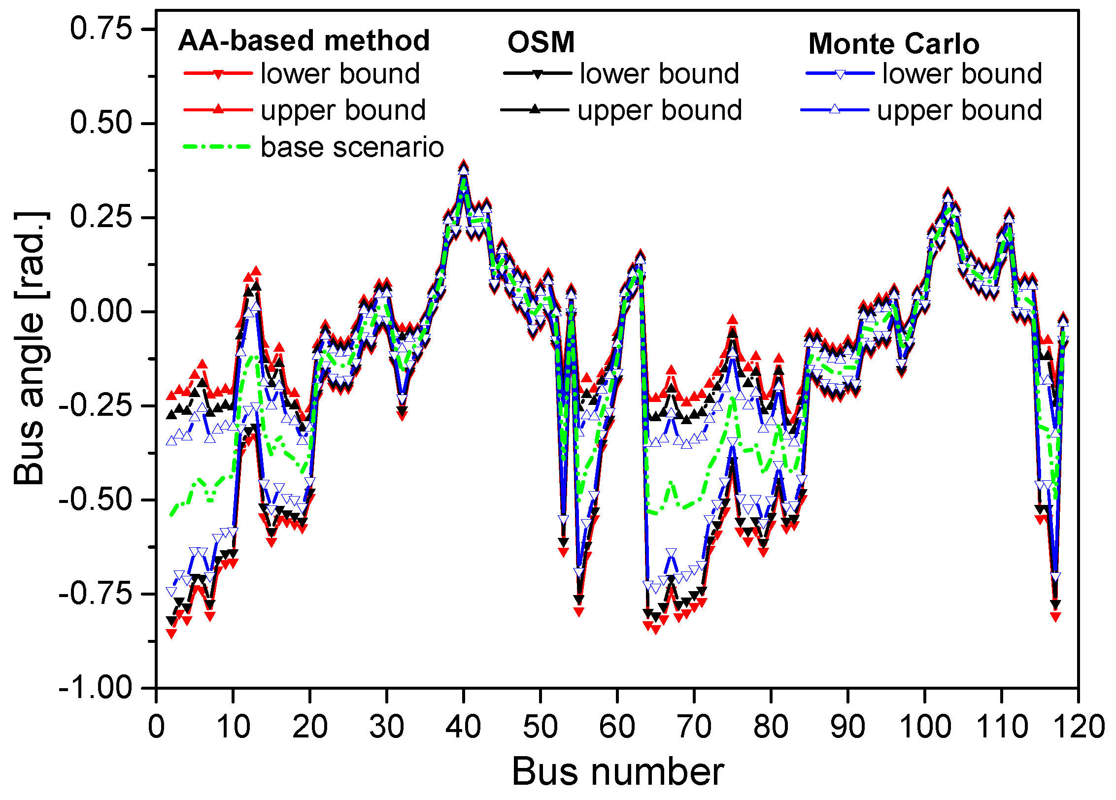
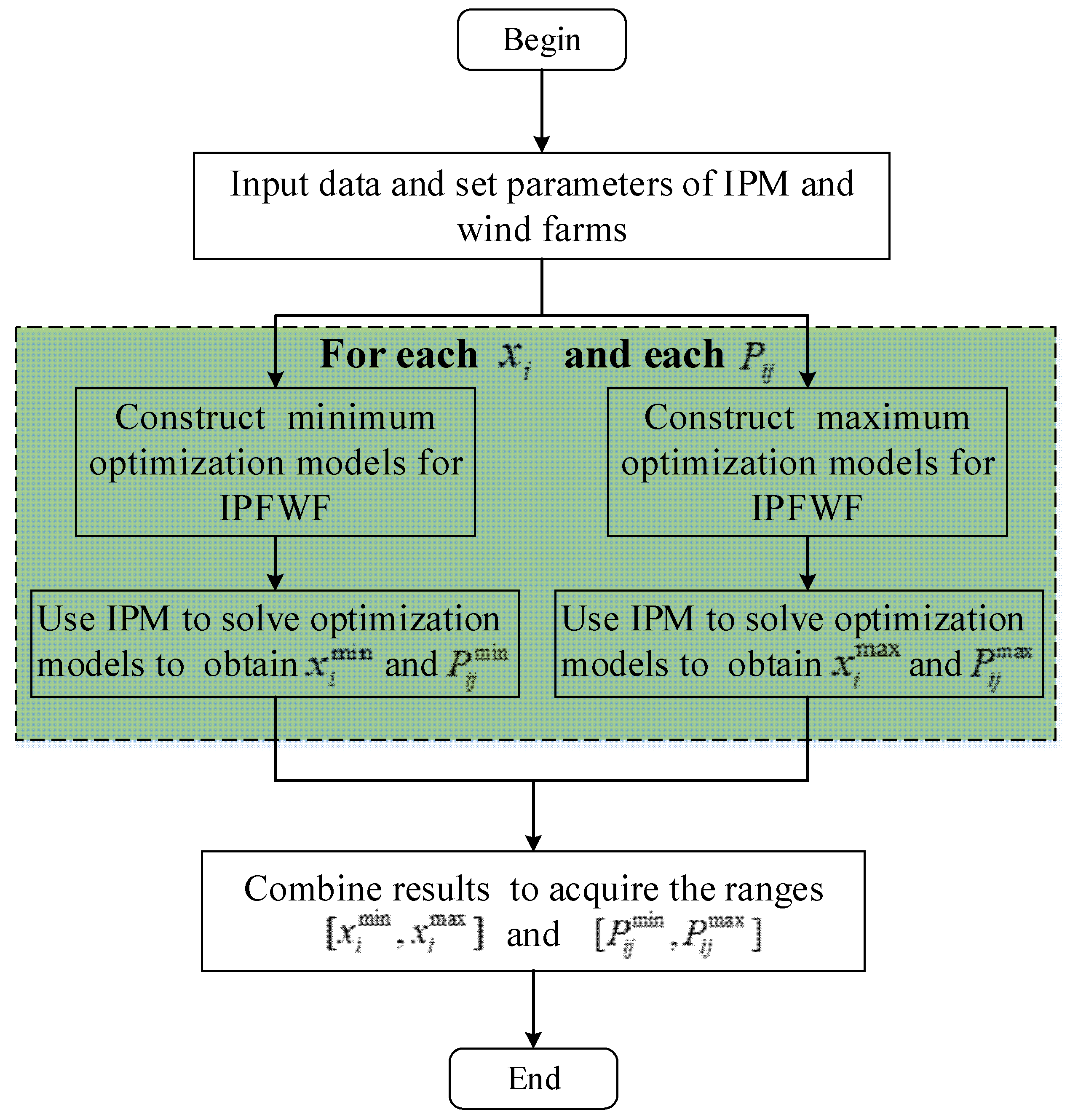
• The OSM was employed here to acquire the intervals of the variables from the IPFWF model. The OSM builds two types of optimization models to acquire ranges of the load voltage magnitudes, bus angles, as well as the active line power flows of the IPFWF model. Three types of constraints of wind control modes were considered in the optimization models of the OSM, so as to imitate the operation features of wind farms. Meanwhile, the voltage recovery processes and limits of reactive power of generators were considered.
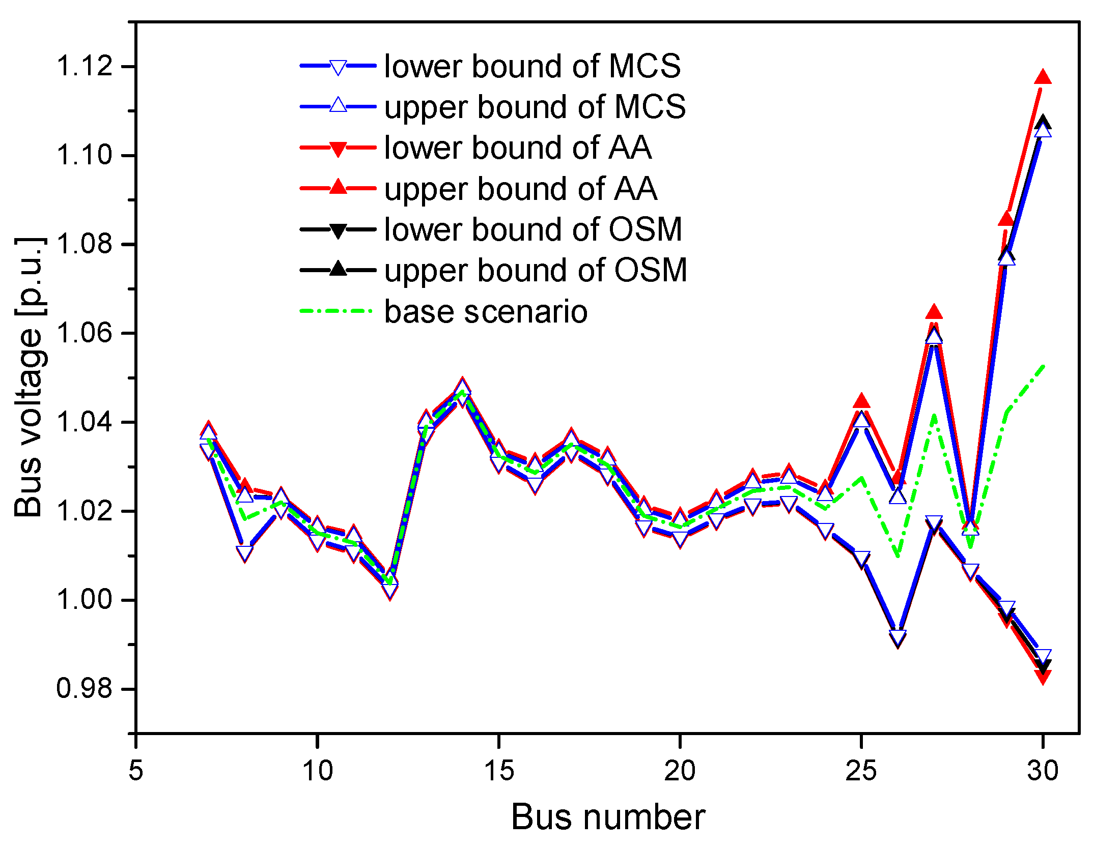
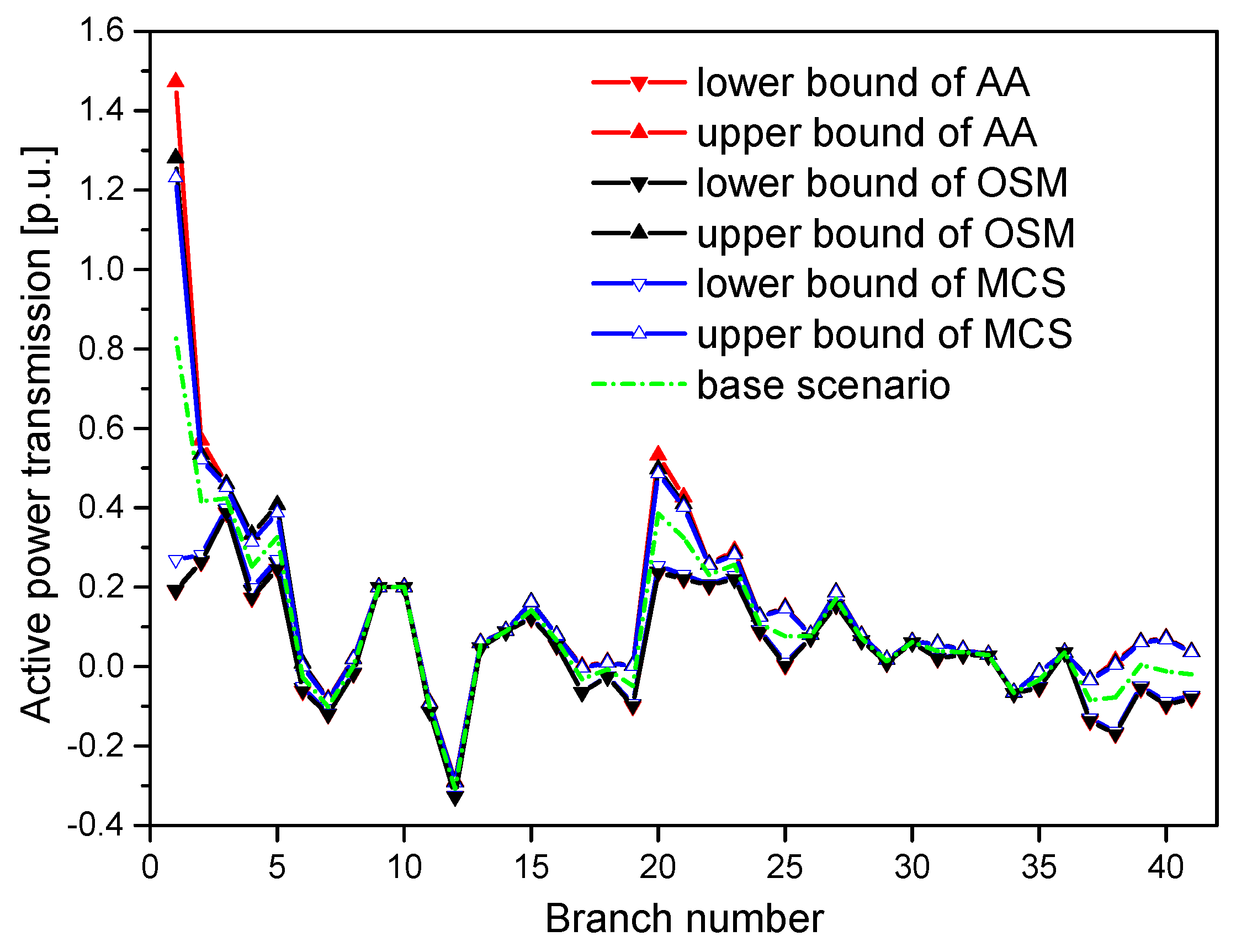
• We compared the results acquired using the AA-based method and OSM in two case studies with those acquired by the MCS, to demonstrate the advantages and effectiveness of the proposed methods, as well as validating their applicability of solving larger systems.

As far as the following contents of this paper are concerned, they are arranged as follows. Mathematical formulations of the IPFWF model are described in Section 2. Introduction of the AA-based method and OSM procedures, which are employed for solving the proposed model, are given in Section 3. Analysis and discussions related to simulation results are introduced in Section 4. The contributions as well as conclusions of the work are introduced in Section 5.

2. Mathematical Formulations of the Problem

2.1. Wind Farm Models

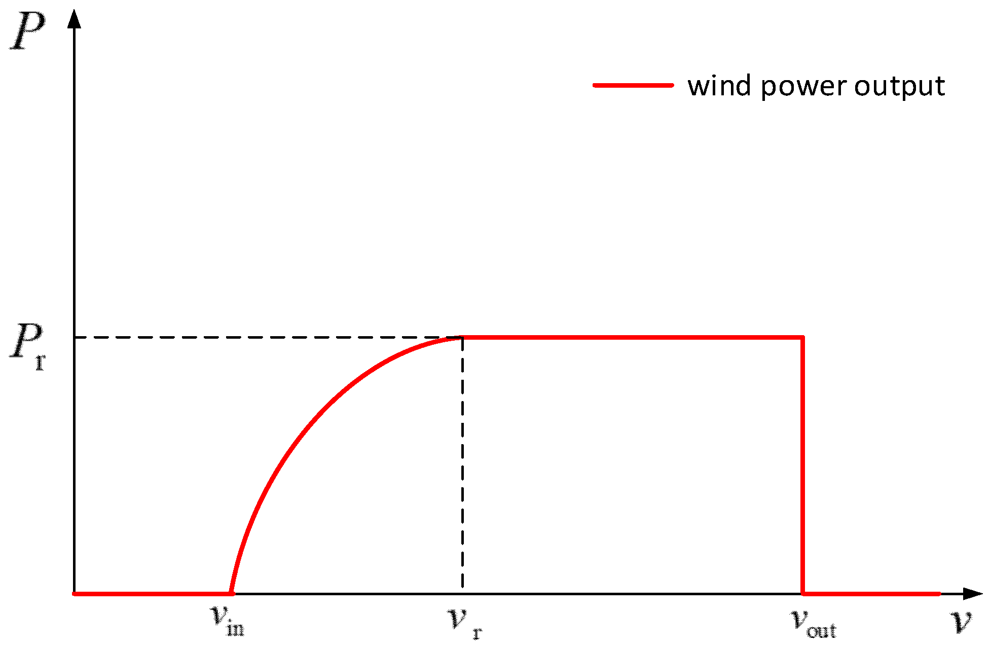
2.1.1. Modeling of the Output Wind Power Generation

Regarding modeling of the wind generators, two kinds of control modes are mainly used for modelling the wind turbines, i.e., fixed speed/constant frequency (FSCF) control and variable speed/constant frequency control (VSFC) [31,32,33]. Variable speed/constant frequency control modes are classified as the constant voltage control mode (CVCM) and the constant power factor control mode (CPFCM) [34,35,36,37]. However, despite the wind turbine’s control types, its output active power should be generally described by functions which vary with wind speeds [38,39]. Generally, a wind farm usually contains numerous wind turbines, whose spatial placement is quite similar because of similarity of landforms. This feature makes the active power outputs of wind turbines in one wind farm show a quite high degree of similarity [40]. Meanwhile, in practice, considering design requirements, relevant control modes are usually employed to control the wind farm’s wind turbines. As a result, a wind farm is able to be regarded as a model of wind turbine if neglecting spacing between turbines, turbulence, and the wake effect [41,42,43].

As is discussed in Reference [44], the output power of wind turbines can be assumed as a function closely related to wind speeds. Numerous expressions have been proposed to present the function relationship between wind speed and output wind power generation, such as quadratic function [44] and cubic function forms [39]. In practice, however, it makes sense to pay more attention to the characteristics of the output power based on the actual operating conditions of wind turbines, rather than the function relationship. Therefore, the cut-out ($v_{co}$), cut-in ($v_{ci}$), and rated ($v_r$) wind speeds should be taken into account when using power generation functions of a wind turbine. Here, we use a formulation proposed in Reference [44], where the output active wind power generation $P_W$ is expressed by a function of wind speeds, and it is given as follows.

$$P_W=\{\begin{array}{l}(A_0+A_{1}v+A_2{v}^2)P_r,\hspace{1em}{v}_{ci}\le v<v_r\\ P_r,\hspace{1em}\hspace{1em}\hspace{1em}\hspace{1em}\hspace{1em}\hspace{1em}\hspace{1em}\hspace{0.17em}{v}_r\le v<v_{co}\\ 0,\hspace{1em}\hspace{1em}\hspace{1em}\hspace{1em}\hspace{1em}\hspace{1em}\hspace{0.17em}\hspace{1em}\hspace{0.17em}\hspace{0.17em}v<v_{ci}\hspace{0.17em}or\hspace{0.17em}v\ge v_{co}\end{array}$$

(1)

where $P_r$ represents rated output active wind power generation and coefficients $A_0$, $A_1$, and $A_2$ are given as follows. The relationship between wind power output and wind speeds is presented Figure 1.

$$\{\begin{array}{l}{A}_2=\frac{1}{{(v_{ci}-v_r)}^2}\left[2-4{\left(\frac{v_{ci}+v_r}{2v_r}\right)}^3\right],\\ A_1=\frac{1}{{(v_{ci}-v_r)}^2}\left[4(v_{ci}+v_r){\left(\frac{v_{ci}+v_r}{2v_r}\right)}^3-(3v_{ci}+v_r)\right],\\ A_0=\frac{1}{{(v_{ci}-v_r)}^2}\left[v_{ci}(v_{ci}+v_r)-4v_{ci}{v}_r{\left(\frac{v_{ci}+v_r}{2v_r}\right)}^3\right].\end{array}$$

(2)

We observe from Equation (1) and Figure 1 that $P_W$ = 0 when $v<v_{ci}\hspace{0.17em}\mathrm{or}\hspace{0.17em}v\ge v_{co}$, and can be written as a quadratic function related to v when $v_{ci}\le v<v_r$. However, $P_W$ is a constant value $P_r$ when $v_r\le v<v_{co}$, due to well adjustable ability of pitch angles of wind turbines. Notice here that $v$ is regarded as a random, and it is with a Weibull distribution:

$$f(v)=\frac{k}{c}{(\frac{v}{c})}^{k-1}\exp \left[-{\left(\frac{v}{c}\right)}^k\right],$$

(3)

where $c$ and $k$, respectively, represent the scale and shape parameters. Therefore, $P_W$ varies in an interval expressed as $[0,P_r]$.

2.1.2. Fixed Speed and Constant Frequency Control

In the initial stage of designing wind turbines, technologies were unable to adjust the speed of impellers for various wind speeds. The active power of wind turbines, therefore, was produced in an asynchronous mode and only over a quite narrow wind speed range. Meanwhile, the PQ and RX nodes were frequently employed by load flow analysis rather than FSCF. Here, Equation (4) will be used for modelling the reactive power consumption of the PQ bus in the FSCF wind turbines.

$$Q=V^2\frac{{\mathrm{X}}_{\mathrm{c}}-{\mathrm{X}}_{\mathrm{m}}}{{\mathrm{X}}_{\mathrm{c}}{\mathrm{X}}_{\mathrm{m}}}+\mathrm{X}\frac{V^2+2\mathrm{R}{P}_W}{2({\mathrm{R}}^2+{\mathrm{X}}^2)}-\mathrm{X}\frac{\sqrt{{(V^2+2\mathrm{R}{P}_W)}^2-4P_W{}^2({\mathrm{R}}^2+{\mathrm{X}}^2)}}{2({\mathrm{R}}^2+{\mathrm{X}}^2)},$$

(4)

where $V$ stands for the bus voltage magnitude, $P_W$ represents the active wind power generation calculated by (1), $\mathrm{R}$ represents the total of the rotor and stator resistance values, $\mathrm{X}$ represents the combination of rotor and stator leakage reactance values, ${\mathrm{X}}_{\mathrm{m}}$ stands for excitation reactance, and ${\mathrm{X}}_{\mathrm{c}}$ stands for the capacitance of shunt capacitors. The principle of power generation is illustrated in Figure 2.

With the development of control technology for wind turbines, FSCF modes became outdated and gradually were substituted by VSCF modes.

2.1.3. Constant Power Factor Control Mode

Constant power factor control mode is a special type of variable speed/constant frequency control mode, and its schematic is illustrated in Figure 3. Here, the current transformer and crowbar resistance are used to realize control of constant power factors. Meanwhile, a resistance here is used to prevent the current from overrunning, and a step-up transformer converts bus voltage to that of the connected grid. As for the reactive power consumption of CPFCM, it is calculated by

$$Q=P_W\times \tan \phi ,$$

(5)

where $\phi$ is the angle of power factor $\cos \phi$ and $P_W$ is the active power generation.

2.1.4. Constant Voltage Control Mode

Constant voltage control mode is another type of variable speed/constant frequency control mode, and its layout is presented in Figure 4. Here, the wind turbine’s voltage can be controlled using the full-power converter operating similar to the thermal generator. In addition, it is able to control its reactive power consumption and is modelled by a PV node.

Based on preceding discussions, the wind turbines in three control modes can be discriminated through distinct reactive power consumption modes. That is, the CVCM is able to control its reactive power output, while the reactive power outputs of FSCF and CPFCM can be calculated through Equations (4) and (5), respectively.

2.2. Interval Power Flow with Wind Farms Model

Regardless of the consideration of wind power, the load flow model of a power grid is expressed as

$$P_{\mathrm{G}i}-P_{\mathrm{L}i}-P_i=0,i\in \left\{\mathrm{generator}\mathrm{buses}\right\},$$

(6)

$$-P_{\mathrm{L}i}-P_i=0,i\in \left\{\mathrm{load}\mathrm{buses}\right\},$$

(7)

$$Q_{\mathrm{C}i}-Q_{\mathrm{L}i}-Q_i=0,i\in \left\{\mathrm{load}\mathrm{buses}\right\},$$

(8)

where

$$Q_i=V_i{\displaystyle \sum _{j\in \mathrm{S}}{V}_j(G_{ij}\sin {\theta }_{ij}-B_{ij}\cos {\theta }_{ij})},$$

(9)

$$P_i=V_i{\displaystyle \sum _{j\in \mathrm{S}}{V}_j(G_{ij}\cos {\theta }_{ij}+B_{ij}\sin {\theta }_{ij})}.$$

(10)

where $\mathrm{S}$ is the set of indices of system buses, $P_{\mathrm{G}i}$ is the $i\mathrm{th}$ generator’s active output power, $Q_{\mathrm{L}i}$ and $P_{\mathrm{L}i}$, respectively, represent reactive and active power load demand of the $i\mathrm{th}$ bus, $Q_{\mathrm{C}i}$ stands for the output of reactive power compensator at the $i\mathrm{th}$ bus, ${\theta }_{ij}={\theta }_i-{\theta }_j$, where ${\theta }_i$ represents the bus angle of the ith bus, and they should regard the slack bus’s angle value as the reference, $V_i$ is the voltage magnitude of the ith bus, $B_{ij}$ and $G_{ij}$ respectively represent the imaginary and real portions of $Y_{ij}$, where $Y=\left\{Y_{ij}\right\}$ is the nodal admittance matrix.

However, if the wind power is taken into consideration, equations of buses related to wind farms should make changes. An obvious change is that all the real power generation of buses with farms should be substituted by intervals, marked as ${\widehat{P}}_{\mathrm{G}i}=[{\underset{\_}{P}}_{\mathrm{G}i},{\overline{P}}_{\mathrm{G}i}]$, where ${\underset{\_}{P}}_{\mathrm{G}i}$ and ${\overline{P}}_{\mathrm{G}i}$ represent minimum and maximum of wind power generation, respectively. Accordingly, the equations of buses correlated to wind farms can be rewritten based on three reactive power control modes in the following. For FSCF wind power control, based on Equation (4), their load flow equations can be rewritten as

$$Q_{\mathrm{G}i}=V_i^2\frac{{\mathrm{X}}_{\mathrm{c}i}-{\mathrm{X}}_{\mathrm{m}i}}{{\mathrm{X}}_{\mathrm{c}i}{\mathrm{X}}_{\mathrm{m}i}}+{\mathrm{X}}_i\frac{V_i^2+2{\mathrm{R}}_i{\widehat{P}}_{\mathrm{G}i}}{2({\mathrm{R}}_i^2+{\mathrm{X}}_i^2)}-{\mathrm{X}}_i\frac{\sqrt{{(V_i^2+2{\mathrm{R}}_i{\widehat{P}}_{\mathrm{G}i})}^2-4{\widehat{P}}_{\mathrm{G}i}^2({\mathrm{R}}_i^2+{\mathrm{X}}_i^2)}}{2({\mathrm{R}}_i^2+{\mathrm{X}}_i^2)},$$

(11)

$${\widehat{P}}_{\mathrm{G}i}-P_{\mathrm{L}i}-P_i=0,$$

(12)

$${\widehat{Q}}_{\mathrm{G}i}-Q_{\mathrm{L}i}-Q_i=0,$$

(13)

the power flow equations of CPFCM control are given by

$${\widehat{Q}}_{\mathrm{G}i}={\widehat{P}}_{\mathrm{G}i}\times \tan \phi ,$$

(14)

$${\widehat{P}}_{\mathrm{G}i}-P_{\mathrm{L}i}-P_i=0,$$

(15)

$${\widehat{Q}}_{\mathrm{G}i}-Q_{\mathrm{L}i}-Q_i=0,$$

(16)

regarding CVCM control buses, it only needs to replace $P_{\mathrm{G}i}$ of Equation (6) with ${\widehat{P}}_{\mathrm{G}i}$:

$${\widehat{P}}_{\mathrm{G}i}-P_{\mathrm{L}i}-P_i=0.$$

(17)

The solution of this interval computation problem will be introduced in the following sections.

3. Solution to the IPFWF Model

3.1. Solution of the IPFWF Model by AA-Based Method

In this section, the AA-based method is employed and modified to solve the IPFWF model [17]. The AA-based method uses the affine arithmetic to realize the interval computation instead of the interval arithmetic, so as to reduce the conservatism of the interval computing results.

3.1.1. Introduction of AA

The affine arithmetic uses a series of noises to express the interval $\widehat{x}=[\underset{\_}{x},\overline{x}]$, which can be written as

$$\widehat{x}=x_0+x_1{\epsilon }_1+x_2{\epsilon }_2+\cdots +x_p{\epsilon }_p,$$

(18)

where ${\epsilon }_i$ stands for a noise element and is valued as interval $[-1,1]$; $x_i$ represents the coefficient corresponding to ${\epsilon }_i$, and it reflects the influence of ${\epsilon }_i$ on the interval $\widehat{x}$; $x_0$ is the midpoint of $\widehat{x}$; $p$ is the number of noise element. The AA form (18) can be easily switched to interval arithmetic form by using formulation

$$\widehat{x}=[x_0-{\displaystyle \sum _{i=1}^p\left|x_i\right|},\hspace{0.17em}{x}_0+{\displaystyle \sum _{i=1}^p\left|x_i\right|}].$$

(19)

where $p$ is the number of noise element, and $\left|x_i\right|$ represents absolute value of $x_i$. Based on the definition (18), the minus/plus and scalar multiplication operators of AA are respectively defined in the following:

$$\widehat{x}\pm \widehat{y}=(x_0\pm y_0)+(x_1\pm y_1){\epsilon }_1+(x_2\pm y_2){\epsilon }_i+\cdots +(x_p+y_p){\epsilon }_p,$$

(20)

$$\alpha \widehat{x}=(\alpha x_0)+(\alpha x_1){\epsilon }_1+(\alpha x_2){\epsilon }_i+\cdots +(\alpha x_p){\epsilon }_p,$$

(21)

where $\alpha$ is a constant. AA-based interval computation is more accurate because the relevance on intervals is considered. For example, $\widehat{x}=[-1,1]$, then $\widehat{x}-\widehat{x}=[-1,1]-[-1,1]=[-2,2]$ according to interval arithmetic, while affine arithmetic leads to computing result as $\widehat{x}-\widehat{x}=(x_0-x_0)+(x_1-x_1){\epsilon }_1=0$. Here, $x_0=0$, $x_1=1$ and ${\epsilon }_1$ is the unique noise element.

However, AA requires more complicated computations on the nonlinear operations. To realize the nonlinear computation, AA needs to linearize the nonlinear functions and introduces new noise elements. If we assume a nonlinear function as $\widehat{z}=f({\epsilon }_1,\hspace{0.17em}{\epsilon }_2,\hspace{0.17em}\cdots ,\hspace{0.17em}{\epsilon }_p)$, then its linear affine arithmetic form can be expressed as

$$f^a({\epsilon }_1,\hspace{0.17em}{\epsilon }_2,\hspace{0.17em}\cdots ,\hspace{0.17em}{\epsilon }_p)={\epsilon }_0+z_1{\epsilon }_1+\hspace{0.17em}{z}_2{\epsilon }_2+\hspace{0.17em}\cdots +z_p{\epsilon }_p+z_k{\epsilon }_k,$$

(22)

where $z_i$$(i=1,2,\dots ,p)$ represents the coefficient of noise element ${\epsilon }_i$ of linear AA form of $\widehat{z}$; ${\epsilon }_k$ is a new noise element; $z_k$ stands for the approximation error caused by linearization of $\widehat{z}$, and it satisfies the following constraint

$$\max \left\{\right|f({\epsilon }_1,\hspace{0.17em}{\epsilon }_2,\hspace{0.17em}\cdots ,\hspace{0.17em}{\epsilon }_p)-f^a({\epsilon }_1,\hspace{0.17em}{\epsilon }_2,\hspace{0.17em}\cdots ,\hspace{0.17em}{\epsilon }_p)|:{\epsilon }_i\in [-1,1]\}\le z_k.$$

(23)

In fact, different linear approximation methods always have different approximation errors, and the Chebyshev function approximation is supposed as the best linear approximation method because it minimizes the approximation errors. Therefore, it is commonly used by AA to compute the intervals of nonlinear function.

3.1.2. Solution of the IPFWF through AA

According to the affine arithmetic theory, the AA-based method is used to solve the IPFWF model. It should be noticed that the FSCF wind farms are not considered in the AA-based method, because it is outdated and is unable to realize affine arithmetic due to complex relationships (11) between active and reactive power. The AA-based method mainly includes three steps, which are introduced in the following.

Step (1) Express the voltage magnitudes of load buses and bus angles of non-slack buses as the following affine forms:

$$V_i=V_{i,0}+{\displaystyle \sum _{j\in \mathrm{CVCM}}{V}_{i,j}^{\mathrm{P}}{\epsilon }_{\mathrm{P}j}}+{\displaystyle \sum _{j\in \mathrm{CPFCM}}{V}_{i,j}^{\mathrm{P}}{\epsilon }_{\mathrm{P}j}}+{\displaystyle \sum _{j\in \mathrm{CPFCM}}{V}_{i,j}^{\mathrm{Q}}{\epsilon }_{\mathrm{Q}j}},\hspace{0.17em}\hspace{0.17em}\mathrm{for}\hspace{0.17em}i\in {\mathrm{S}}_{\mathrm{L}},$$

(24)

$${\theta }_i={\theta }_{i,0}+{\displaystyle \sum _{j\in \mathrm{CVCM}}{\theta }_{i,j}^{\mathrm{P}}{\epsilon }_{\mathrm{P}j}}+{\displaystyle \sum _{j\in \mathrm{CPFCM}}{\theta }_{i,j}^{\mathrm{P}}{\epsilon }_{\mathrm{P}j}}+{\displaystyle \sum _{j\in \mathrm{CPFCM}}{\theta }_{i,j}^{\mathrm{Q}}{\epsilon }_{\mathrm{Q}j}},\hspace{0.17em}\hspace{0.17em}\mathrm{for}\hspace{0.17em}i\in {\mathrm{S}}_{\mathrm{G}}\cup {\mathrm{S}}_{\mathrm{L}},$$

(25)

where coefficients $V_{i,j}^{\mathrm{P}}$, $V_{i,j}^{\mathrm{Q}}$, ${\theta }_{i,j}^{\mathrm{P}}$, ${\theta }_{i,j}^{\mathrm{Q}}$ are partial deviations corresponding to noise elements ${\epsilon }_{\mathrm{P}j}$, ${\epsilon }_{\mathrm{Q}j}$. Here, these coefficients should be enlarged by an amplification to ensure (24) and (25) include the real ranges of bus angles and load voltage magnitudes. $V_{i,0}$ and ${\theta }_{i,0}$ are load voltage magnitude and bus angle results at nominal point. Because CPFCM wind farms satisfy constraint (14), then ${\epsilon }_{\mathrm{Q}j}={\epsilon }_{\mathrm{P}j}\times \tan {\phi }_j$. Therefore, (24) and (25) are rewritten as

$$V_i=V_{i,0}+{\displaystyle \sum _{j\in \mathrm{CVCM}}{V}_{i,j}^{\mathrm{P}}{\epsilon }_{\mathrm{P}j}}+{\displaystyle \sum _{j\in \mathrm{CPFCM}}(V_{i,j}^{\mathrm{P}}+V_{i,j}^{\mathrm{Q}}\tan {\phi }_j){\epsilon }_{\mathrm{P}j}},\hspace{0.17em}\hspace{0.17em}\mathrm{for}\hspace{0.17em}i\in {\mathrm{S}}_{\mathrm{L}}.$$

(26)

$${\theta }_i={\theta }_{i,0}+{\displaystyle \sum _{j\in \mathrm{CVCM}}{\theta }_{i,j}^{\mathrm{P}}{\epsilon }_{\mathrm{P}j}}+{\displaystyle \sum _{j\in \mathrm{CPFCM}}({\theta }_{i,j}^{\mathrm{P}}+{\theta }_{i,j}^{\mathrm{Q}}\tan {\phi }_j){\epsilon }_{\mathrm{P}j}},\hspace{0.17em}\hspace{0.17em}\mathrm{for}\hspace{0.17em}i\in {\mathrm{S}}_{\mathrm{G}}\cup {\mathrm{S}}_{\mathrm{L}}.$$

(27)

Step (2) Substitute the affine forms of voltage magnitude and bus angles into power flow equations, thus compute the affine forms of injected active power and reactive power, which are written as

$${\widehat{P}}_i=P_{i,0}+{\displaystyle \sum _{j\in \mathrm{CVCM}\cup \mathrm{CPFCM}}{P}_{i,j}^{\mathrm{P}}{\epsilon }_{\mathrm{P}j}}+{\displaystyle \sum _{h\in nN}{P}_{i,h}{\epsilon }_h},\hspace{0.17em}\hspace{0.17em}\mathrm{for}\hspace{0.17em}i\in {\mathrm{S}}_{\mathrm{G}}\cup {\mathrm{S}}_{\mathrm{L}},$$

(28)

$${\widehat{Q}}_i=Q_{i,0}+{\displaystyle \sum _{j\in \mathrm{CVCM}\cup \mathrm{CPFCM}}{Q}_{i,j}^{\mathrm{P}}{\epsilon }_{\mathrm{P}j}}+{\displaystyle \sum _{h\in nN}{Q}_{i,h}{\epsilon }_h},\hspace{0.17em}\hspace{0.17em}\mathrm{for}\hspace{0.17em}i\in {\mathrm{S}}_{\mathrm{L}},$$

(29)

where $Q_{i,0}$ and $P_{i,0}$ are respective the injected reactive and active power for buses without wind farms, for buses with wind farms,

$$P_{i,0}=\frac{{\underset{\_}{P}}_{\mathrm{G}i}+{\overline{P}}_{\mathrm{G}i}}{2}(i\in \mathrm{CVCM}\cup \mathrm{CPFCM})$$

(30)

and

$$Q_{i,0}=\frac{{\underset{\_}{P}}_{\mathrm{G}i}+{\overline{P}}_{\mathrm{G}i}}{2}\tan {\phi }_i(i\in \mathrm{CPFCM}).$$

(31)

$nN$ is the set of new noise variables caused by affine approximation computations, which include multiplication and Chebyshev linear approximation for sine and cosine functions. Here, the approximation computation is conducted according to the constraint (23).

Step (3) Construct linear programming problems to contract the ranges of noise symbols ${\epsilon }_{\mathrm{P}i}$. Based on the affine forms expressed by (28) and (29), we can acquire the following matrix form:

$$f(X)=AX+B,$$

(32)

where

$$X={[{\epsilon }_1\hspace{0.17em}{\epsilon }_2\hspace{0.17em}\cdots \hspace{0.17em}{\epsilon }_N]}^T,$$

(33)

$$f(X)=\left[\begin{array}{l}\widehat{\mathit{P}}\\ \widehat{\mathit{Q}}\end{array}\right],$$

(34)

$$\widehat{\mathit{Q}}={[{\widehat{Q}}_1\hspace{0.17em}{\widehat{Q}}_2\cdots {\widehat{Q}}_{nQ}]}^T,$$

(35)

$$\widehat{\mathit{P}}={[{\widehat{P}}_1\hspace{0.17em}{\widehat{P}}_2\cdots {\widehat{P}}_{nP}]}^T,$$

(36)

$$A=\left[\begin{array}{l}\begin{array}{ccc}{P}_{1,1}^P& \cdots & P_{1,N}^P\\ \cdots & \cdots & \cdots \\ P_{nP,1}^P& \cdots & P_{nP,N}^P\end{array}\\ \begin{array}{ccc}{Q}_{1,1}^P& \cdots & Q_{1,N}^P\\ \cdots & \cdots & \cdots \\ Q_{nQ,1}^P& \cdots & Q_{nQ,N}^P\end{array}\end{array}\right],$$

(37)

$$B=\left[\begin{array}{c}\begin{array}{c}{P}_{1,0}\\ \cdots \\ P_{nQ,0}\end{array}\\ \begin{array}{c}{Q}_{1,0}\\ \cdots \\ Q_{nP,0}\end{array}\end{array}\right]+\left[\begin{array}{c}\begin{array}{ccc}{P}_{1,1}& \cdots & P_{1,nN}\\ \cdots & \cdots & \cdots \\ P_{nP,1}& \cdots & P_{nP,nN}\end{array}\\ \begin{array}{ccc}{Q}_{1,1}& \cdots & Q_{1,nN}\\ \cdots & \cdots & \cdots \\ Q_{nQ,1}& \cdots & Q_{nQ,nN}\end{array}\end{array}\right]\left[\begin{array}{c}\begin{array}{c}{\epsilon }_1\\ \cdots \\ \cdots \end{array}\\ \begin{array}{c}\cdots \\ \cdots \\ {\epsilon }_{nN}\end{array}\end{array}\right],$$

(38)

$nP$ and $nQ$ are the element number of sets ${\mathrm{S}}_{\mathrm{G}}\cup {\mathrm{S}}_{\mathrm{L}}$ and ${\mathrm{S}}_{\mathrm{L}}$. Here, $X$ represents the vector of noise elements that should be contracted, and the initial value of each dimension is set as the interval [−1,1]; $A$ is a matrix that consists of calculated real parameters; $B$ is an interval vector computed by the new noise elements. Because the newly produced noise element ${\epsilon }_h$ varies within a fixed interval [−1,1] and cannot be contracted, and they stand for the internal noise elements introduced by the nonlinear function’s AA computational process.

Since the ranges of (32) will contain the ranges of the real ranges of injected nodal power, due to multiplication of amplification coefficients on the partial deviations of voltage magnitude and bus angles affine forms in step (1), as well as usage of affine approximation computations in step (2). Therefore, the intervals of load flow variables are acquired through compressing the ranges of vector $X$ such that

$$AX+B=f^{SP},$$

(39)

where $f^{SP}$ represents a vector valued by intervals, which are defined by the fixed ranges of reactive and active power inputs. To contract the vector $X$, the “min” and “max” linear programming problems are established as follows, respectively:

$$\begin{array}{l}\min {\epsilon }_{Pj}\hspace{1em}\mathrm{or}\hspace{0.17em}\hspace{0.17em}\max {\epsilon }_{Pj},\hspace{0.17em}\mathrm{for}\hspace{0.17em}j\in \mathrm{CVCM}\cup \mathrm{CPFCM}\\ s.t.\{\begin{array}{l}-1\le {\epsilon }_{Pj}\le 1\\ \inf (C_i)\le {\displaystyle \sum _{j\in \mathrm{CVCM}\cup \mathrm{CPFCM}}{A}_{ij}{\epsilon }_{Pj}}\le \sup (C_i),i=1,2,\cdots ,nP+nQ\end{array}\end{array}$$

(40)

where $C=f^{SP}-B$; $\inf (\cdot )$ and $\sup (\cdot )$ are infimum and supremum functions. By solving (32), the accurate ranges of bus angles and voltage magnitudes are acquired as follows:

$$\{\begin{array}{l}{V}_i=V_{i,0}+{\displaystyle \sum _{j\in \mathrm{CVCM}}{V}_{i,j}^{\mathrm{P}}[{\epsilon }_{\mathrm{P}j,\min },{\epsilon }_{\mathrm{P}j,\max }]}+{\displaystyle \sum _{j\in \mathrm{CPFCM}}(V_{i,j}^{\mathrm{P}}+V_{i,j}^{\mathrm{Q}}\tan {\phi }_j)[{\epsilon }_{\mathrm{P}j,\min },{\epsilon }_{\mathrm{P}j,\max }]},\hspace{0.17em}\hspace{0.17em}\mathrm{for}\hspace{0.17em}i\in {\mathrm{S}}_{\mathrm{L}}\\ {\theta }_i={\theta }_{i,0}+{\displaystyle \sum _{j\in \mathrm{CVCM}}{\theta }_{i,j}^{\mathrm{P}}[{\epsilon }_{\mathrm{P}j,\min },{\epsilon }_{\mathrm{P}j,\max }]}+{\displaystyle \sum _{j\in \mathrm{CPFCM}}({\theta }_{i,j}^{\mathrm{P}}+{\theta }_{i,j}^{\mathrm{Q}}\tan {\phi }_j)[{\epsilon }_{\mathrm{P}j,\min },{\epsilon }_{\mathrm{P}j,\max }]},\hspace{0.17em}\hspace{0.17em}\mathrm{for}\hspace{0.17em}i\in {\mathrm{S}}_{\mathrm{G}}\cup {\mathrm{S}}_{\mathrm{L}}\end{array}$$

(41)

After the three steps, the intervals of voltage magnitudes and bus angles are obtained. To obtain (28) and (29), some affine approximation computations like multiplication and Chebyshev approximation need to be done, and detailed information about how to do these approximation computations can be found in Reference [20]. To make it easier to understand the AA-based method, a simple case study is employed and introduced in detail in the Appendix A section.

3.2. Solution of the IPFWF Model by OSM

In this section, the solution process of the proposed IPFWF model through the OSM is discussed. The OSM is mainly proposed through the extreme value theorem [32]. To make a comprehension of the OSM, introduction of extreme value theorem as well as two vital viewpoints are given as follows.

(Extreme Value Theorem): Assume that $f$ is a real-valued continuous function bounded in a closed interval $[a,b]$, then $f$ must obtain at least one minimum and one maximum. In other words, there are real numbers $d$ and $c$ in $[a,b]$ satisfying $f(d)\le f(x)\le f(c)$ for arbitrary $x\in [a,b]$.

Then, for brevity, we express the IPFWF model as $\mathit{h}(\mathit{x})=[{\mathit{h}}^{\mathrm{L}},{\mathit{h}}^{\mathrm{U}}]$, where ${\mathit{h}}^{\mathrm{L}}$ and ${\mathit{h}}^{\mathrm{U}}$, respectively, represent lower and upper bounds of the injected power, for the buses without wind farms ${\mathit{h}}^{\mathrm{L}}={\mathit{h}}^{\mathrm{U}}$, and $\mathit{x}$ are power flow variables including bus angles and load voltage magnitudes. According to the extreme value theory, the two key points can be expressed as follows.

Viewpoint 1: For each scenario $\mathit{\xi }\in [{\mathit{h}}^{\mathrm{L}},{\mathit{h}}^{\mathrm{U}}]$, there exists a fixed $\mathit{x}$ which corresponds to $\mathit{\xi }$, and this relationship is established by load flow equations. That is to say, $\mathit{x}$ varies with uncertain $\mathit{\xi }$.

Viewpoint 2: For every dimension $x_i$ of $\mathit{x}$, there is a selected scenario ${\mathit{\xi }}_{\max }^{(i)}$ making $x_i$ maximum for arbitrary scenario $\mathit{\xi }\in [{\mathit{h}}^{\mathrm{L}},{\mathit{h}}^{\mathrm{U}}]$. Meanwhile, there exists a specific scenario ${\mathit{\xi }}_{\min }^{(i)}$, which makes minimum. If we respectively mark the maximum and minimum values as $x_i^{\max }$ and $x_i^{\min }$, then $[x_i^{\min },x_i^{\max }]$ is the varying interval of $x_i$ under the active wind power generation data interval $[{\mathit{h}}^{\mathrm{L}},{\mathit{h}}^{\mathrm{U}}]$, this is because the function $\mathit{y}=\mathit{h}(\mathit{x})$ is continuous and the extreme theorem takes effects here.

It is known from Viewpoint 2 that the solution of the IPFWF model is reduced to searching the extreme scenarios ${\mathit{\xi }}_{\max }^{(i)}$ and ${\mathit{\xi }}_{\min }^{(i)}$ for every $x_i$. Accordingly, we can regard $\mathit{\xi }$ as variables bounded by interval $[{\mathit{h}}^{\mathrm{L}},{\mathit{h}}^{\mathrm{U}}]$, and establish two optimization models to obtain the variation interval of $x_i$. Based on the extreme value theorem, the OSM establishes the maximum and minimum programming models to acquire intervals of the power flow results of the IPFWF model, and they can be formulated as follows.

$$\mathrm{minimize}\hspace{0.17em}{x}_i\hspace{1em}\mathrm{or}\hspace{1em}\mathrm{maxmum}\hspace{0.17em}{x}_i$$

(42)

s.t.

$$\{\begin{array}{l}{P}_{\mathrm{G}i}-P_{\mathrm{L}i}-P_i=0,\hspace{0.17em}i\in \{\mathrm{generator}\hspace{0.17em}\mathrm{buses}\}\\ \hspace{1em}\hspace{0.17em}-P_{\mathrm{L}i}-P_i=0,\hspace{0.17em}i\in \{\mathrm{load}\hspace{0.17em}\mathrm{buses}\}\\ Q_{\mathrm{C}i}-Q_{\mathrm{L}i}-Q_i=0,\hspace{0.17em}i\in \{\mathrm{load}\hspace{0.17em}\mathrm{buses}\}\end{array}$$

(43)

and

$$\{\begin{array}{l}{\xi }_i-P_{\mathrm{L}i}-P_i=0,\hspace{0.17em}i\in \{\mathrm{FSFT}\hspace{0.17em}\mathrm{or}\hspace{0.17em}\mathrm{CPFCM}\hspace{0.17em}\mathrm{or}\hspace{0.17em}\mathrm{CVCM}\}\\ Q_{\mathrm{G}i}-Q_{\mathrm{L}i}-Q_i=0,\hspace{0.17em}i\in \{\mathrm{FSFT}\hspace{0.17em}\mathrm{or}\hspace{0.17em}\mathrm{CPFCM}\}\\ Q_{\mathrm{G}i}=V_i^2\frac{{\mathrm{X}}_{\mathrm{c}i}-{\mathrm{X}}_{\mathrm{m}i}}{{\mathrm{X}}_{\mathrm{c}i}{\mathrm{X}}_{\mathrm{m}i}}+{\mathrm{X}}_i\frac{V_i^2+2{\mathrm{R}}_i{\widehat{P}}_{\mathrm{G}i}}{2({\mathrm{R}}_i^2+{\mathrm{X}}_i^2)}-{\mathrm{X}}_i\frac{\sqrt{{(V_i^2+2{\mathrm{R}}_i{\widehat{P}}_{\mathrm{G}i})}^2-4{\widehat{P}}_{\mathrm{G}i}^2({\mathrm{R}}_i^2+{\mathrm{X}}_i^2)}}{2({\mathrm{R}}_i^2+{\mathrm{X}}_i^2)},\hspace{0.17em}i\in \{\mathrm{FSFT}\}\\ Q_{\mathrm{G}i}={\widehat{P}}_{\mathrm{G}i}\times \tan \phi ,\hspace{0.17em}i\in \left\{\mathrm{CPFCM}\right\}\\ {\underset{\_}{P}}_{\mathrm{G}i}\le {\xi }_i\le {\overline{P}}_{\mathrm{G}i},\hspace{0.17em}i\in \{\mathrm{FSFT}\hspace{0.17em}\mathrm{or}\hspace{0.17em}\mathrm{CPFCM}\hspace{0.17em}\mathrm{or}\hspace{0.17em}\mathrm{CVCM}\}\end{array}$$

(44)

where $x_i$ represents the variables of power flow equations, which can be $V_i$ or ${\theta }_i$, and ${\xi }_i$ is a variable constrained in the interval $[{\underset{\_}{P}}_{\mathrm{G}i},{\overline{P}}_{\mathrm{G}i}]$. If the ranges of the active transmission power flow are considered, the expression

$$P_{ij}=V_i{V}_j(G_{ij}\cos {\theta }_{ij}+B_{ij}\sin {\theta }_{ij})-G_{ij}{V}_i^2$$

(45)

should replace $x_i$ in Reference (18), where $P_{ij}$ represents the active line power transmitted from bus $i$ to bus $j$. Here, the real portion of the shunt admittances is neglected for simplifying the computation of $P_{ij}$. In addition, if we consider limits on the voltage recovery processes and reactive power generation of the generators within these programs, and these constraints are listed as

$$V_i-V_{\mathrm{G}i}-V_{ai}+V_{bi}=0,\hspace{0.17em}\hspace{0.17em}i\in \{\mathrm{generator}\hspace{0.17em}\mathrm{buses}\},$$

(46)

$$(Q_{\mathrm{G}i}-Q_{\mathrm{G}i}^{\min })V_{ai}=0,\hspace{0.17em}\hspace{0.17em}i\in \{\mathrm{generator}\hspace{0.17em}\mathrm{buses}\},$$

(47)

$$(Q_{\mathrm{G}i}^{\max }-Q_{\mathrm{G}i})V_{bi}=0,\hspace{0.17em}\hspace{0.17em}i\in \{\mathrm{generator}\hspace{0.17em}\mathrm{buses}\},$$

(48)

$$Q_{\mathrm{G}i}=Q_{\mathrm{L}i}+Q_i,\hspace{0.17em}\hspace{0.17em}i\in \{\mathrm{generator}\hspace{0.17em}\mathrm{buses}\},$$

(49)

$$Q_{\mathrm{G}i}^{\min }\le Q_{\mathrm{G}i}\le Q_{\mathrm{G}i}^{\max },\hspace{0.17em}\hspace{0.17em}i\in \{\mathrm{generator}\hspace{0.17em}\mathrm{buses}\},$$

(50)

$$V_{ai},V_{bi}\ge 0,\hspace{0.17em}\hspace{0.17em}i\in \{\mathrm{generator}\hspace{0.17em}\mathrm{buses}\}.$$

(51)

where $V_{bi}$ and $V_{ai}$ represent the slack variables for tracking the variation of the voltage magnitudes, $V_{\mathrm{G}i}$ stands for the initial point value of the voltage at the generator bus $i$, $Q_{\mathrm{G}i}^{\max }$ and $Q_{\mathrm{G}i}^{\min }$ are the upper and lower limitations of the reactive power generation $Q_{\mathrm{G}i}$, respectively.

The solution models expressed by Equations (42)–(44) are all nonlinear optimization models, and they could be solved efficiently using the interior point method (IPM) [45]. According to the established optimization models, we illustrate the procedure for solving the IPFWF model in Figure 5. Here, the input data include network parameters, injected active power and voltage of the generator buses, and injected power of load buses. Parameters of the wind farms mainly consist of their cut-in, cut-out, rated wind speeds, rated output power, as well as the Weibull distribution information of wind speeds. Parameters of IPM contain the iteration precision and the central parameter.

4. Simulation Results

Two test cases will be navigated in this section, including the IEEE 30-bus and IEEE 118-bus systems. Case one will simulate the IEEE 30-bus system, and results acquired using the AA-based method and OSM are compared with those obtained suing the MCS method in this case, thus demonstrating the advantages and effectiveness of the proposed two methods. The second case is used to demonstrate the applicability of the proposed methods for handling larger systems, where the IEEE 118-bus will be simulated and analyzed. Network parameters of IEEE 118-bus and IEEE 30-bus systems are introduced in detail elsewhere [46]. One-hundred MV A was selected as the test systems’ basic power, and all parameters and data were computed in per-unit (p.u.) system. The constant power factor of CPFCM was $\cos \phi =0.95$. To facilitate an easier description of the results, all the bus orders of the test systems were rearranged with the reference (slack) bus first, followed in order by the buses connected to the CVCM wind farm, conventional generator buses, load buses (capacitor buses prior), and finally buses combined with the CPFCM wind farm. The order of all branches was also rearranged, the rear bus number of the branch was set larger than that of its front bus number. The whole branches were arranged in an ascending order based on the number of the front bus, where, if the number of the front bus in two branches were identical, the branch with a bigger rear bus number would be set in a front order. Accordingly, real transmission power was calculated from its front bus to its rear bus. The IPM’s central parameter was set as 0.1, and iteration precision was chosen as ${10}^{-6}$. Sampling numbers of MCS in two cases were both set as 5000, and this number was large enough for ensuring the accuracy of sampling results. To show the possible fluctuations of the power system state as a function of uncertain wind farms generation, the “base scenario” was given in all figures which describes the variables’ intervals of IPFWF models. Here, the base scenario was defined as the obtained power flow results when the wind power outputs of wind farms equals to the midpoint of their variation intervals.

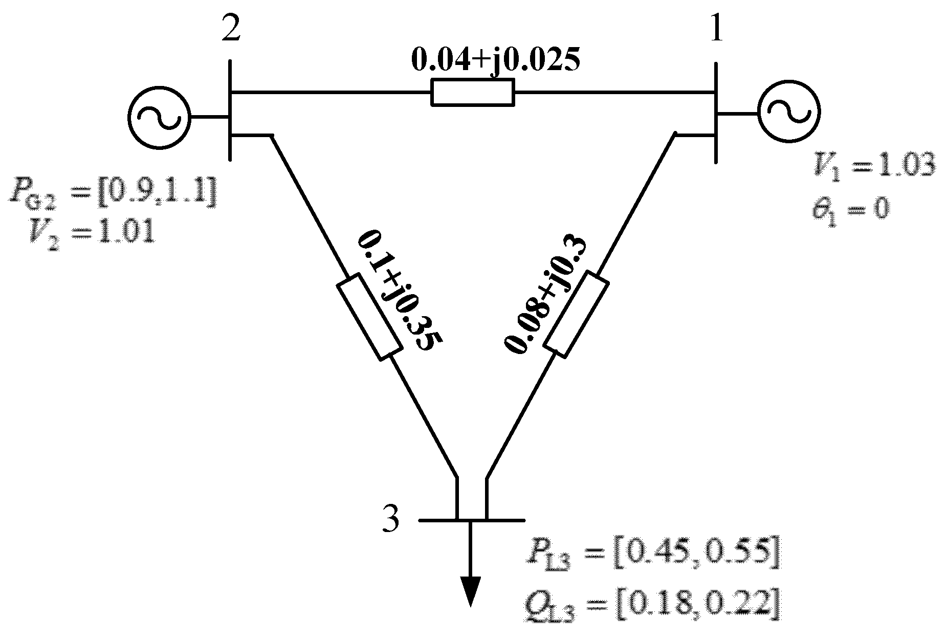
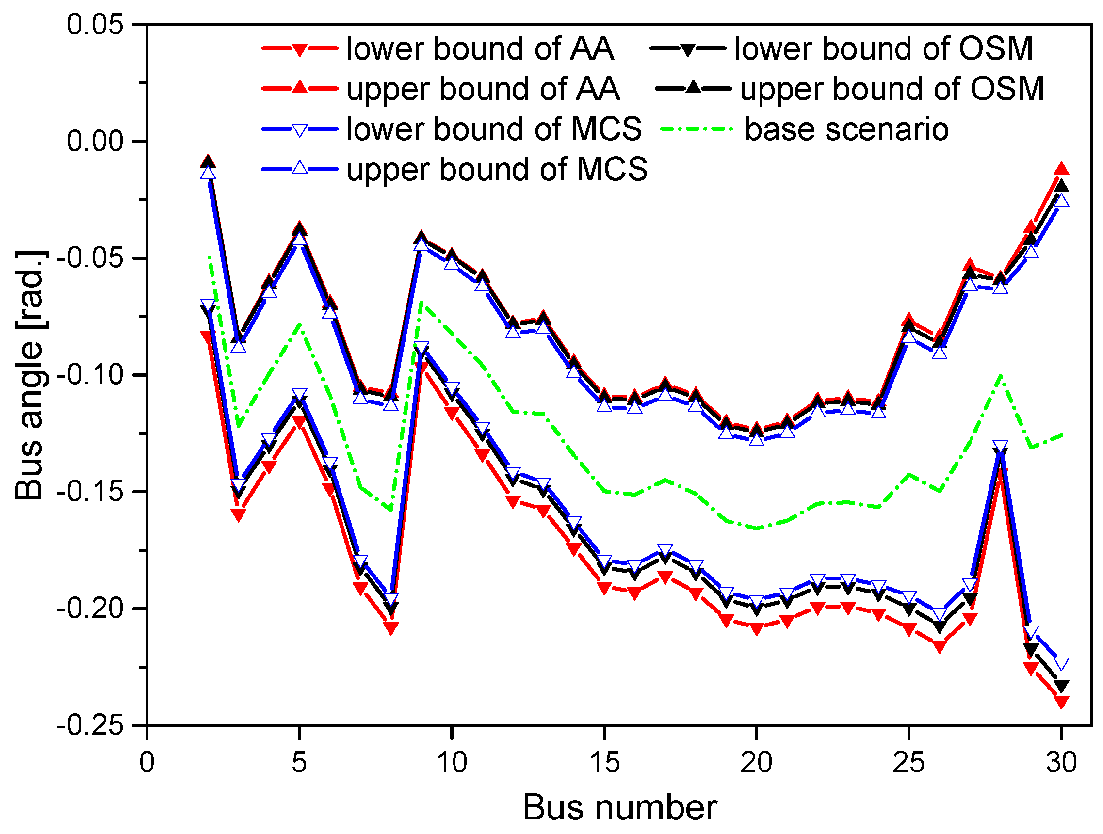
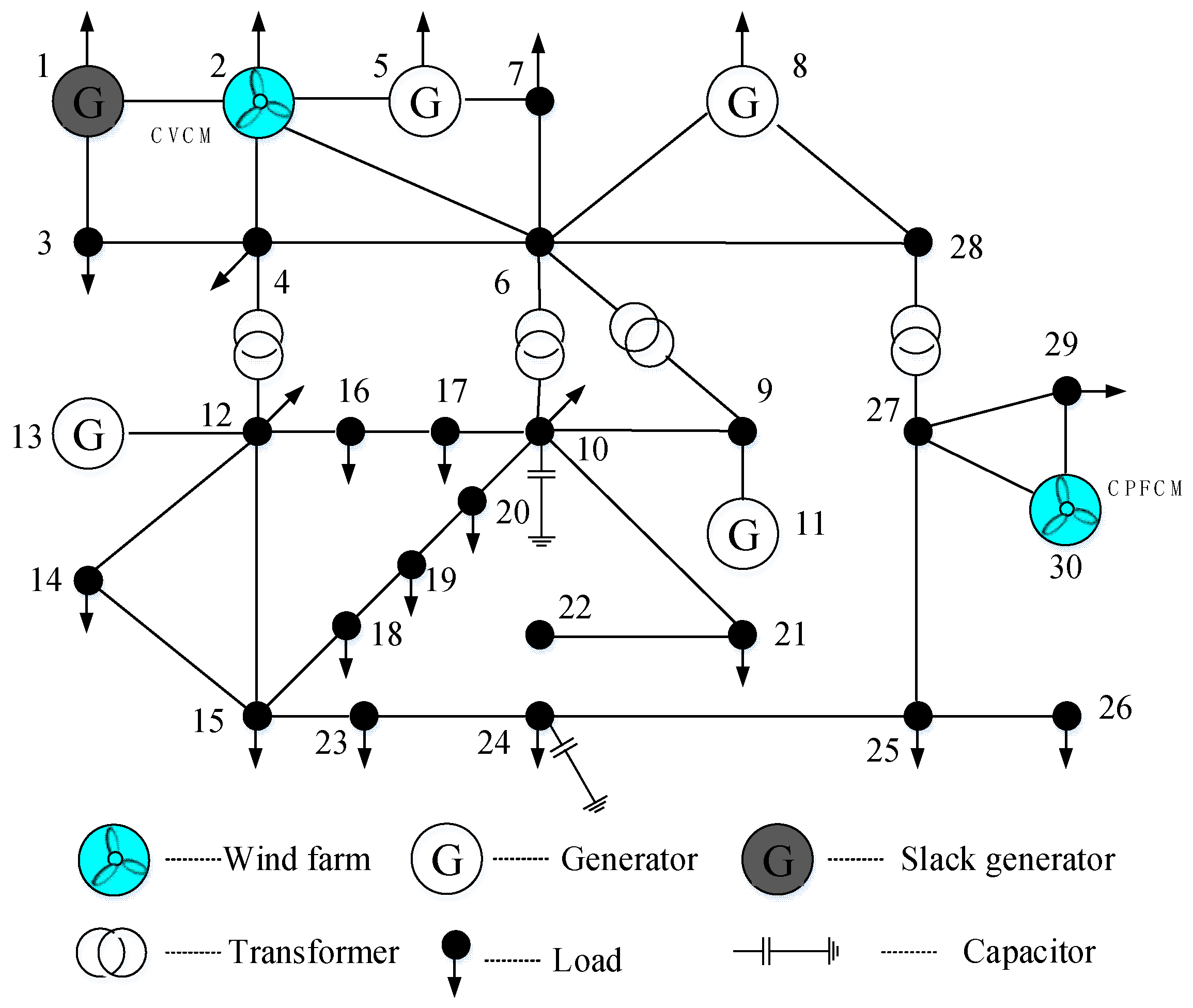
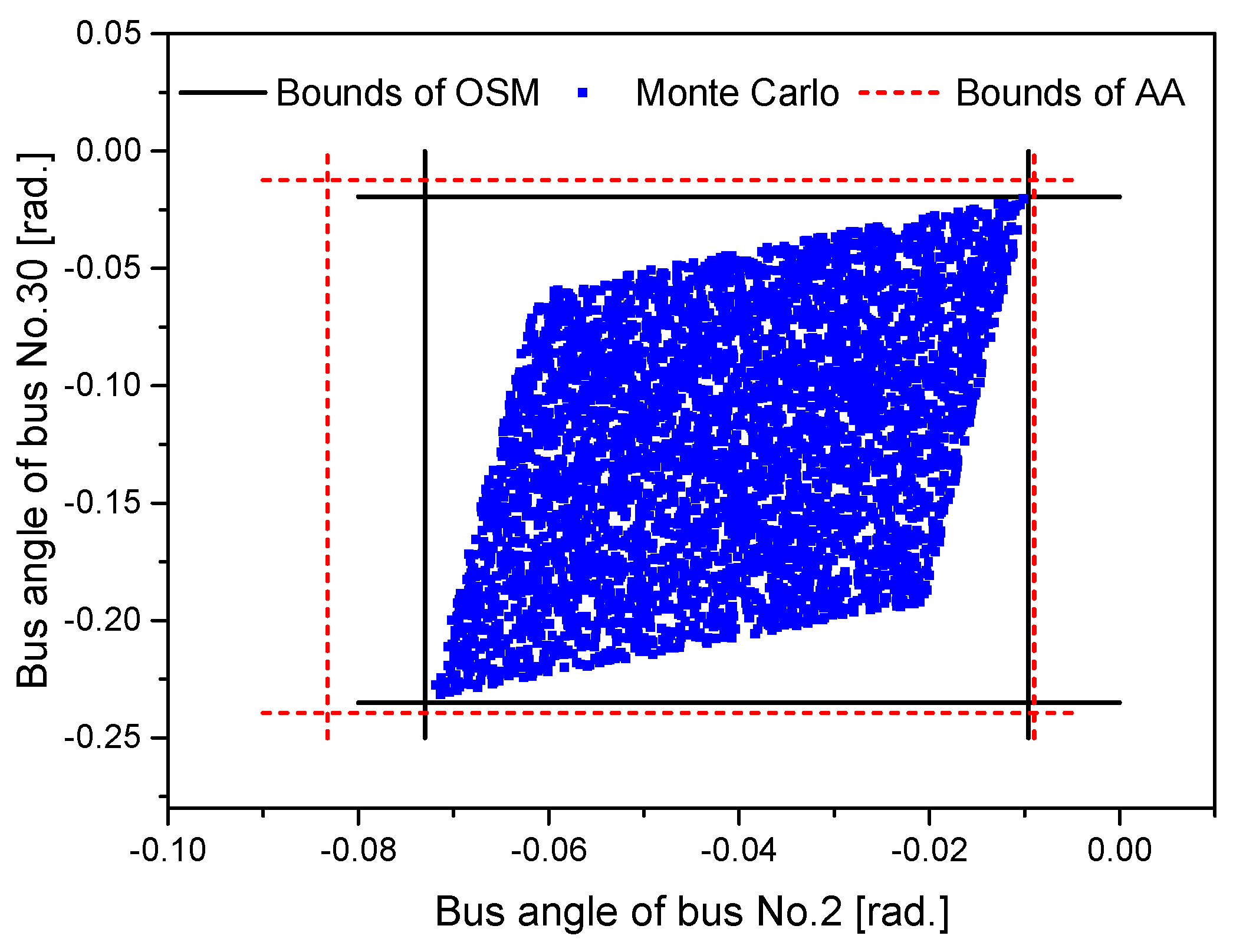
4.1. IEEE 30-Bus System

The IEEE 30-bus system was modified and tested here to demonstrate the advantages and effectiveness of the OSM in addressing the IPFWF model by comparing with the MCS. This system contains 37 transmission lines, five generators, two capacitors, four transformers, and two wind farms, see Figure 6. Here, the generator at bus No. 2 and load bus No. 30 were modified as wind farms. The positions of the wind farms in CPFCM and CVCM control modes were respectively located on buses No. 2 and No. 30. Intervals of input power data of the CPFCM and CVCM wind farms were given as [0, 0.2756] (p.u.) and [0, 1.04] (p.u.), respectively. Limits of reactive power of the generators were given as [−0.5, 1] (p.u.). The active power generation of power compute through (1)–(3), and the Weibull distribution parameters of wind speeds as well as the operational parameters of the wind turbines are presented in

Table 1. Wind farm rated power and wind speed parameters.

Type	Pr (MW)	c	k	vco (m/s)	vr (m/s)	vci (m/s)
CPFCM	27.56	7.5	2	20	14	5
CVCM	104	8	2	24	16	4

CPFCM and CVCM respectively stands for the wind farms in constant voltage control mode and the constant power factor control mode.

.

According to the aforementioned parameters and input data, the proposed IPFWF model is solved by the MCS, AA-based method, and OSM. The load voltage, bus angle, and active transmission power results are exhibited in Figure 7, Figure 8 and Figure 9, respectively. Notice that load flow variable results acquired using the OSM and the AA-based method are broader than those acquired through the MCS. This is because the MCS is unable to consider the whole scenarios when producing samples. However, the AA-based method mainly relies on affine arithmetic computation, which represents a kind of self-validated computation, and it always obtains more conservative results than “real” results due to approximation errors produced by affine arithmetic computation of nonlinear functions. The OSM considers all probable scenarios due to usage of the interval, which includes the whole extreme scenarios described through the upper and lower bounds, and it was proven to acquire the most accurate interval results [25]. To show this inclusion relationship of these three methods more clearly, the sampling results of bus angles at bus No. 30 and bus No. 2 are exhibited in Figure 10. Observe that all MCS samples bounded in intervals acquired using the OSM, while interval bounds of OSM reside in those of in the AA-based method. In Figure 7 and Figure 8, it shows that load voltage at bus No. 30, bus angle at bus No. 2, and bus angle of bus No. 30 all display huge fluctuations because bus No. 2 and bus No. 30 are related to wind farms. In Figure 9, the transmission power of branch No. 1 also fluctuates widely because it connects bus No. 1 (the slack bus) with bus No. 2, which is related with a CVCM wind farm.

The results and analysis of this case demonstrate that the OSM and the AA-based method could provide an effective approach to addressing the IPFWF model. Meanwhile, the comparing results indicate that results acquired by the OSM are more accurate than those obtained using the MCS and the AA-based method.

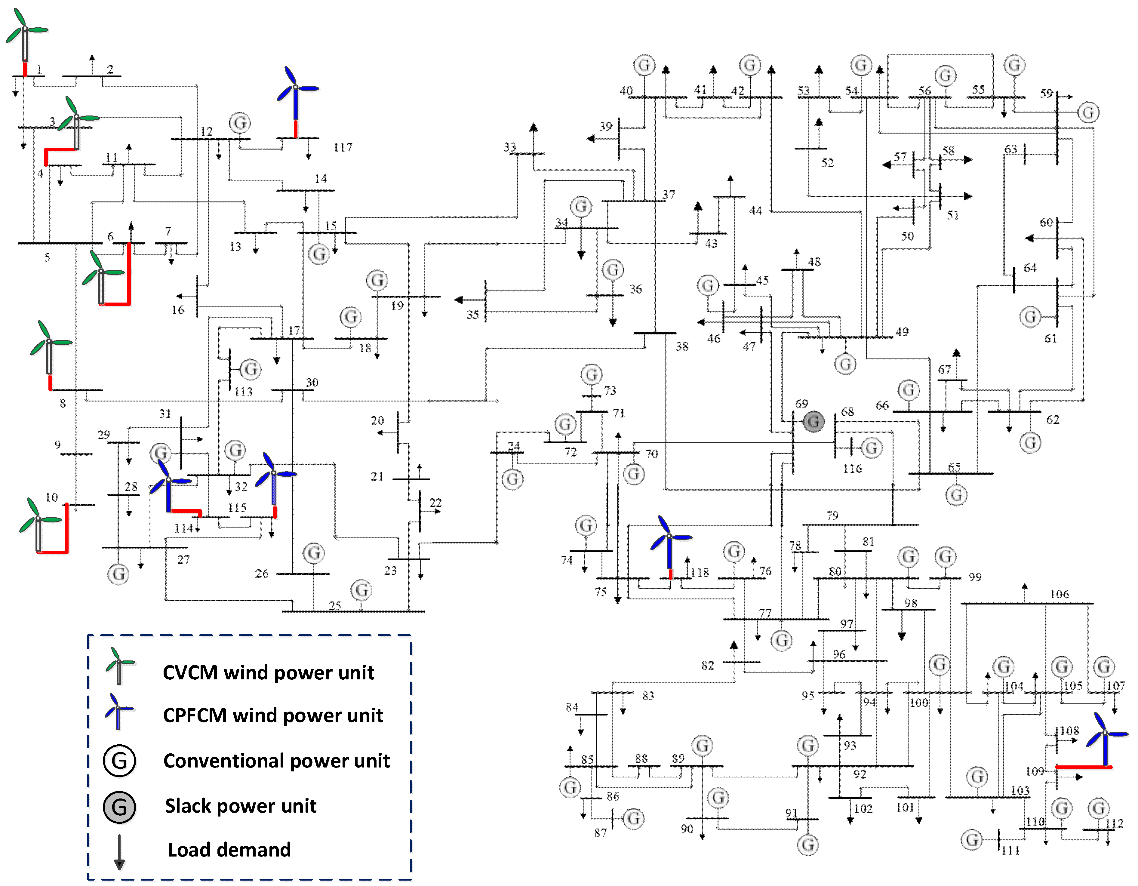
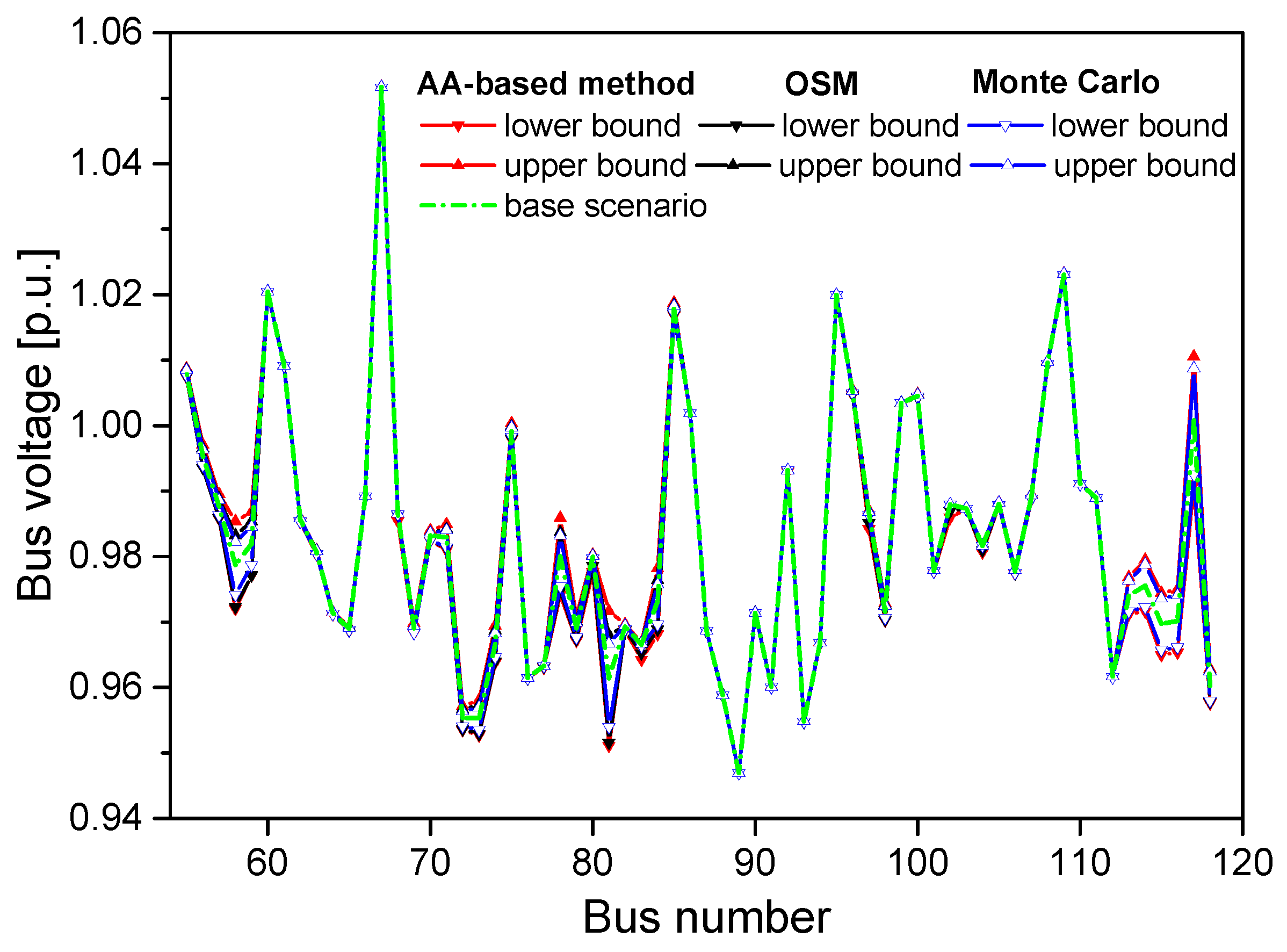
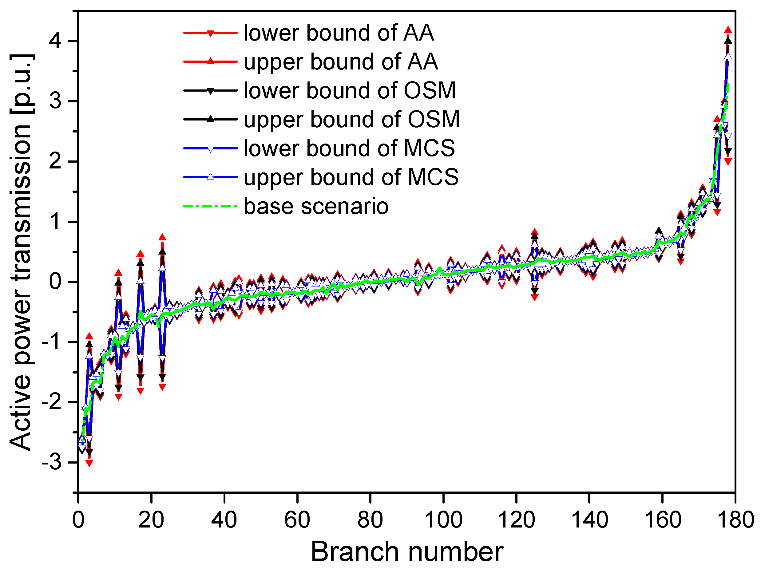
4.2. IEEE 118-Bus System

The IEEE 118-bus contains 169 lines, 9 transformers, 54 generator buses, and 9 capacitors (see Figure 11). To account for the wind farms, the IEEE 118-bus system is modified and connected to CVCM and CPFCM wind farms. Here, generators at bus Nos. 1, 4, 6, 8, and 10 are set as CVCM wind farms and load bus Nos. 109, 114, 115, 117, and 118 are transformed as CPFCM wind farms, and their parameters are listed in

Table 2. Parameters of wind speed and wind farms in the IEEE 118-bus system.

Bus Position	Type	${\mathit{v}}_{\mathit{c}\mathit{i}}(\mathbf{m}/\mathbf{s})$	${\mathit{v}}_{\mathit{r}}(\mathbf{m}/\mathbf{s})$	${\mathit{v}}_{\mathit{c}\mathit{o}}(\mathbf{m}/\mathbf{s})$	${\mathit{P}}_{\mathit{r}}\left(\mathbf{MW}\right)$	k	c
1	CVCM	5	14	20	50	2	7.5
4	CVCM	6	15	24	50	3	8
6	CVCM	4	16	21.5	50	2.5	8.0
8	CVCM	4	17	23	50	2.5	7.5
10	CVCM	4	15	24	50	2	8.5
109	CPFCM	5	14	21	21.2	2	7.5
114	CPFCM	4	16	22	21.2	2.5	6.5
115	CPFCM	6	16	23	21.2	2	8.5
117	CPFCM	5.5	16	24	21.2	2.5	7.5
118	CPFCM	5	15	20	21.2	3	7.0

. This table includes the information of bus positions, control types, wind speeds, rated output power, and parameters of their Weibull distributions.

Based on the aforementioned data and parameters, the IEEE 118 bus system is solved by the OSM, AA-based method, and MCS. The bus angles, load voltages, and the active transmission powers are respectively presented in Figure 12, Figure 13 and Figure 14. In Figure 14, the branches are reordered according to the midpoint values of the active transmission power intervals. Observe from the data and figures that the interval results acquired by these three methods still hold the inclusion relationship in Case one, which furthermore validates the explanations for different accuracy. Besides, greater fluctuations on the bus angles, voltage magnitudes, as well as the transmission power usually occur on the buses with farms or the branches connected to buses with wind farms. This is expected because fluctuations on injected power of buses is bound to cause the fluctuations on bus angles, bus voltages, and transmission power rated to these buses. This case validates the applicability of the proposed methods to large bus systems.

Regarding the required computational time, both cases were tested through MATLAB 2016b on a 3.2 GHz CPU and 4 G RAM. Testing of the modified IEEE 30-bus system by the AA-based method, OSM, and MCS, respectively, required 4 s, 5 s, and 20 s, while IEEE 118-bus system needed 15 s, 25 s, and 50 s. It indicates that the computational efficiency of the AA-based method and the OSM is much less than that of MCS. To show the applicability of the AA-based method and the OSM to real systems, we tested the Polish 2383-bus system. We found that the AA-based method was able to solve the Polish 2383-bus system within 1 h, whereas the OSM could not work out results in one day. This is because the solution models of the OSM are non-convex nonlinear programming problems, which are time-consuming especially when the scale of the problem grows large.

5. Conclusions

This paper used intervals to express the active power outputs of wind farms, and accordingly proposed the IPFWF model for obtaining load flow results of power grids incorporating uncertain wind power. Meanwhile, the IPFWF model uses three different formulations to describe three control modes of wind farms. The OSM and the AA-based method were employed to solve the proposed IPFWF model. The AA-based method expressed the wind power data intervals as affine arithmetic forms, and constructs optimization models to contract the affine arithmetic forms and obtain the accurate intervals of power flow variables. The OSM solved the IPFWF model through switching its solution to two types of optimization models that could be efficiently addressed using the IPM. To show the advantages, effectiveness, and applicability of the proposed methods for solving the IPFWF model, the IEEE 30-bus and IEEE 118-bus test systems were tested. Results of testing the IEEE 30-bus system indicate that the AA-based method and the OSM were effective for solving the IPFWF model, and it also demonstrated that the OSM can obtain more accurate results than the MCS method and AA-based method. The case of testing the IEEE 118-bus system showed that the OSM and the AA-based method outperformed the MCS in terms of required computational time, which demonstrates the proposed two methods’ good applicability to larger systems.

The ranges obtained by the AA-based method are always wider than the “real” ranges of the IPFWF model, because its solution process includes Chebyshev approximation errors when computing affine forms of nonlinear functions. However, the approximation errors can be further reduced through defining higher orders of affine forms. The OSM is able to obtain the accurate results of the IPFWF model, but the optimization models established in its solution process belong to nonlinear programmes, and its solution obtained by the IPM is not necessary to be global solution, which may cause the underestimation of the interval results of the IPFWF model. Therefore, further work is needed to relax the nonlinear programmes to convex problems, so as to seek more reliable but accurate solutions to the IPFWF model.

References

1. Li, Z.; Ye, L.; Zhao, Y.; Song, X.; Teng, J.; Jin, J. Short-term wind power prediction based on extreme learning machine with error correction. Prot. Control Mod. Power Syst. 2016, 1, 1–8. [Google Scholar] [CrossRef]
2. Chen, Y.; Wen, J.; Cheng, S. Probabilistic load flow method based on Nataf transformation and Latin hypercube sampling. IEEE. Sustain. Energy 2013, 4, 294–301. [Google Scholar] [CrossRef]
3. Zhou, G.; Bo, R.; Chien, L.; Zhang, X.; Yang, S.; Su, D. GPU-Accelerated Algorithm for On-line probabilistic power flow. IEEE Trans. Power Syst. 2018, 33, 1132–1135. [Google Scholar] [CrossRef]
4. Hong, Y.Y.; Lin, F.J.; Yu, T.H. Taguchi method-based probabilistic load flow studies considering uncertain renewables and loads. IET Renew. Power Gener. 2016, 10, 221–227. [Google Scholar] [CrossRef]
5. Yuan, Y.; Zhou, J.; Ju, P. Probabilistic load flow computation of a power system containing wind farms using the method of combined cumulants and Gram-Charlier expansion. IET Renew. Power Gener. 2011, 5, 448–454. [Google Scholar] [CrossRef]
6. Fan, M.; Vittal, V.; Heydt, G.T. Probabilistic power flow studies for transmission systems with photovoltaic generation using cumulants. IEEE Trans. Power Syst. 2012, 27, 2251–2261. [Google Scholar] [CrossRef]
7. Williams, T.; Crawford, C. Probabilistic load flow modeling comparing maximum entropy and Gram-Charlier probability density function reconstructions. IEEE Trans. Power Syst. 2013, 28, 272–280. [Google Scholar] [CrossRef]
8. Xiao, Q.; He, Y.; Chen, K.; Yang, Y.; Lu, Y. Point estimate method based on univariate dimension reduction model for probabilistic power flow computation. IET Gener. Trans. Distrib. 2017, 11, 3522–3531. [Google Scholar] [CrossRef]
9. Saunders, C.S. Point estimate method addressing correlated wind power for probabilistic optimal power flow. IEEE Trans. Power Syst. 2014, 29, 1045–1054. [Google Scholar] [CrossRef]
10. Liu, C.; Sun, K.; Wang, B. Probabilistic power flow analysis using multi-dimensional Holomorphic embedding and generalized cumulants. IEEE Trans. Power Syst. 2018, 33, 7132–7142. [Google Scholar] [CrossRef]
11. Zhang, L.; Cheng, H.; Zhang, S. A novel point estimate method for probabilistic power flow considering correlated nodal power. In Proceedings of the 2014 IEEE PES General Meeting|Conference & Exposition, National Harbor, MD, USA, 27–31 July 2014; pp. 1–5. [Google Scholar]
12. Aien, M.; Khajeh, M.G.; Rashidinejad, M. Probabilistic power flow of correlated hybrid wind-photovoltaic power systems. IET Renew. Power Gener. 2014, 8, 649–658. [Google Scholar] [CrossRef]
13. Zuluaga, C.D.; Alvarez, M.A. Bayesian probabilistic power flow analysis using Jacobian approximate Bayesian computation. IEEE Trans. Power Syst. 2018, 33, 5217–5225. [Google Scholar] [CrossRef]
14. Yu, H.; Rosehart, B. Probabilistic power flow considering wind speed correlation of wind farms. In Proceedings of the 17th Power Systems Computation Conference, Stockholm, Sweden, 22–26 August 2011; pp. 1–7. [Google Scholar]
15. Hajian, M.; Rosehart, W.D.; Zareipour, H. Probabilistic power flow by Monte Carlo simulation with Latin supercube sampling. IEEE Trans. Power Syst. 2013, 28, 1550–1559. [Google Scholar] [CrossRef]
16. Baghaee, H.R.; Mirsalim, M.; Gharehpetian, G.B. Fuzzy unscented transform for uncertainty quantification of correlated wind/PV microgrids: Possibilistic–probabilistic power flow based on RBFNNs. IET Renew. Power Gener. 2017, 11, 867–877. [Google Scholar] [CrossRef]
17. Melhorn, A.C.; Dimitrovski, A. Three-phase probabilistic load flow in radial and meshed distribution networks. IET Gener. Trans. Distrib. 2015, 9, 2743–2750. [Google Scholar] [CrossRef]
18. Wang, Z.; Alvarado, F.L. Interval arithmetic in power flow analysis. IEEE Trans. Power Syst. 1992, 7, 1341–1349. [Google Scholar] [CrossRef] [Green Version]
19. Mori, H.; Yuihara, A. Calculation of multiple power flow solutions with the Krawczyk method. In Proceedings of the 1999 IEEE International Symposium on Circuits and Systems VLSI (Cat. No.99CH36349), Orlando, FL, USA, 30 May–2 June 1999; pp. 94–97. [Google Scholar]
20. De Figueiredo, L.H.; Stolfi, J. Affine arithmetic: Concepts and applications. Numer. Algorithm. 2004, 37, 147–158. [Google Scholar] [CrossRef]
21. Vaccaro, A.; Canizares, C.; Villacci, D. An affine arithmetic-based methodology for reliable power flow analysis in the presence of data uncertainty. IEEE Trans. Power Syst. 2010, 25, 624–632. [Google Scholar] [CrossRef]
22. Pirnia, M.; Canizares, C.A.; Bhattacharya, K.; Vaccaro, A. An affine arithmetic method to solve the stochastic power flow problem based on a mixed complementarity formulation. In Proceedings of the 2012 IEEE Power and Energy Society General Meeting, San Diego, CA, USA, 22–26 July 2012; pp. 1–7. [Google Scholar]
23. Vaccaro, A.; Cañizares, C.A.; Bhattacharya, K. A range arithmetic-based optimization model for power flow analysis under interval uncertainty. IEEE Trans. Power Syst. 2013, 28, 1179–1186. [Google Scholar] [CrossRef]
24. Zhang, C.; Chen, H.; Ngan, H.; Yang, P.; Hua, D. A mixed interval power flow analysis under rectangular and polar coordinate system. IEEE Trans. Power Syst. 2017, 32, 1422–1429. [Google Scholar] [CrossRef]
25. Zhang, C.; Chen, H.; Shi, K.; Qiu, M.; Hua, D.; Ngan, H. An interval power flow analysis through optimizing-scenarios method. IEEE Trans. Smart Grid 2018, 9, 5217–5226. [Google Scholar] [CrossRef]
26. Zhang, C.; Chen, H.; Guo, M.; Wang, X.; Liu, Y.; Hua, D. DC power flow analysis incorporating interval input data and network parameters through the optimizing-scenarios method. Int. J. Electr. Power Energy Syst. 2018, 96, 380–389. [Google Scholar] [CrossRef]
27. Ran, X.; Miao, S. Three-phase probabilistic load flow for power system with correlated wind, photovoltaic and load. IET Gener. Transm. Distrib. 2016, 10, 3093–3101. [Google Scholar] [CrossRef]
28. Li, X.; Cao, J.; Lu, P. Probabilistic load flow computation in power system including wind farms with correlated parameters. In Proceedings of the 2nd IET Renewable Power Generation Conference (RPG 2013), Beijing, China, 9–11 September 2013; pp. 1–4. [Google Scholar]
29. Jaoued, I.B.; Guesmi, T.; Abdallah, H.H. Power flow solution for power systems including FACTS devices and wind farms. In Proceedings of the IEEE International Conference on Sciences and Technology of Automatic Control and Computer Engineering, Sousse, Tunisia, 7 April 2014; pp. 136–139. [Google Scholar]
30. Vaccaro, A.; Canizares, C.A. An affine arithmetic-based framework for uncertain power flow and optimal power flow studies. IEEE Trans. Power Syst. 2016, 32, 274–288. [Google Scholar] [CrossRef]
31. Zhang, C.; Chen, H.; Ngan, H. Reactive power optimisation considering wind farms based on an optimal scenario method. IET Gener. Transm. Distrib. 2016, 10, 3736–3744. [Google Scholar] [CrossRef]
32. Jin, X.; Zhang, C.; Chen, H.; Xu, X. Optimal reactive power dispatch considering wind turbines. In Proceedings of the 2014 IEEE PES Asia-Pacific Power and Energy Engineering Conference (APPEEC), Hong Kong, China, 7–10 December 2014; pp. 1–5. [Google Scholar]
33. Castro, L.M.; Fuerte-Esquivel, C.R.; Tovar-Hernandez, J.H. A unified approach for the solution of power flows in electric power systems including wind farms. Electr. Power Syst. Res. 2011, 81, 1859–1865. [Google Scholar] [CrossRef]
34. Feijoo, A.; Villanueva, D. Wind farm power distribution function considering wake effects. IEEE Trans. Power Syst. 2017, 32, 3313–3314. [Google Scholar] [CrossRef]
35. Shi, L.B.; Weng, Z.X.; Yao, L.Z. An analytical solution for wind farm power output. IEEE Trans. Power Syst. 2014, 29, 3122–3123. [Google Scholar] [CrossRef]
36. Priyadharshini, P.; Mohamed, T.A.M. Modeling and analysis of wind farms in load flow studies. In Proceedings of the 2015 International Conference on Computation of Power, Energy, Information and Communication (ICCPEIC), Chennai, India, 22–23 April 2015; pp. 364–372. [Google Scholar]
37. Feijoo, A.; Villanueva, D. Four parameter models for wind farm power curves and power probability density functions. IEEE Trans. Sustain. Energy 2017, 8, 1783–1784. [Google Scholar] [CrossRef]
38. Eminoglu, U.; Ayasun, S. Modeling and design optimization of variable-speed wind turbine systems. Energies 2014, 7, 402–419. [Google Scholar] [CrossRef]
39. Eminoglu, U. A new model for output power calculation of variable-speed wind turbine systems. In Proceedings of the 2015 International Aegean Conference on Electrical Machines & Power Electronics (ACEMP), Side, Turkey, 2–4 September 2015; pp. 141–146. [Google Scholar]
40. Sulaeman, S.; Benidris, M.; Mitra, J. A method to model the output power of wind farms in composite system reliability assessment. In Proceedings of the 2014 North American Power Symposium (NAPS), Pullman, WA, USA, 7–9 September 2014; pp. 1–6. [Google Scholar]
41. Yu, H.; Rosehart, W.D. An optimal power flow algorithm to achieve robust operation considering load and renewable generation uncertainties. IEEE Trans. Power Syst. 2012, 27, 1808–1817. [Google Scholar] [CrossRef]
42. Merizalde, Y.; Bonilla, L.M.; Hernández-Callejo, L.; Duque-Perez, O. Wind turbine maintenance. A review. DYNA-Ingeniería e Industria 2018, 93, 435–441. [Google Scholar] [CrossRef]
43. Tian, J.; Su, C.; Soltani, M. Active power dispatch method for a wind farm central controller considering wake effect. In Proceedings of the IECON 2014—40th Annual Conference of the IEEE Industrial Electronics Society, Dallas, TX, USA, 29 October–1 November 2014; pp. 5450–5456. [Google Scholar]
44. Ghosh, S.; Kamalasadan, S.; Senroy, N. Doubly fed induction generator (DFIG)-based wind farm control framework for primary frequency and inertial response application. IEEE Trans. Power Syst. 2016, 31, 1861–1871. [Google Scholar] [CrossRef]
45. Liu, M.; Tso, S.K.; Cheng, Y. An extended nonlinear primal-dual interior-point algorithm for reactive-power optimization of large-scale power systems with discrete control variables. IEEE Trans. Power Syst. 2002, 17, 982–991. [Google Scholar] [CrossRef]
46. Power Systems Test Case Archive. Available online: http://www.ee.washington.edu/research/pstca/ (accessed on 3 January 2018).
Figure 1. Relationship between wind power output and wind speeds according to Equation (1).
Energies 11 03176 g001
Figure 2. Simplified circuit of fixed speed/constant frequency type wind turbines.
Energies 11 03176 g002
Figure 3. Schematic of a constant power factor control mode wind turbine.
Energies 11 03176 g003
Figure 4. Schematic of a constant voltage control mode wind turbine.
Energies 11 03176 g004
Figure 5. Solution process of solving the interval power flow considering wind farm (IPFWF) model based on the optimizing-scenarios method (OSM).
Energies 11 03176 g005
Figure 6. Layout of IEEE 30-bus system incorporating constant power factor control mode (CPFCM) and constant voltage control mode (CVCM) wind farms.
Energies 11 03176 g006
Figure 7. Ranges of bus angles acquired by three different methods.
Energies 11 03176 g007
Figure 8. Ranges of load voltages acquired by three different methods.
Energies 11 03176 g008
Figure 9. Ranges of active transmission power by three different methods.
Energies 11 03176 g009
Figure 10. Sampling results of bus angles at bus No. 2 and bus No. 30.
Energies 11 03176 g010
Figure 11. Layout of the IEEE 118 bus system with different wind power farms.
Energies 11 03176 g011
Figure 12. Bus angle results obtained by different methods.
Energies 11 03176 g012
Figure 13. Load voltage magnitude results obtained by different methods.
Energies 11 03176 g013
Figure 14. Results of active transmission power obtained by different methods.
Energies 11 03176 g014