1. Introduction
The electromagnetic transients program (EMTP) has been widely used for real-time simulation of power systems [
1], verifying the control strategy [
2], and detecting the operational status [
3]. However, one of the limitations of conventional EMTP-type simulators is their inability of performing efficient simulations. The scale of power systems is expanding [
4], and the efficiency of electromagnetic transient simulations cannot meet the needs of scientific tests and theoretical research.
The concept of “diakoptics” was first introduced by Kron in the 1950s [
5]. Kron’s diakoptics was aimed at the solution of large power system networks with increased computational speeds. Jose.R.Marti proposed the MATE concept in order to solve the network in partitioned form [
6]. The main philosophy of MATE is to split the solution of a large system into the solution of a number of smaller subsystems, plus the solution of the links joining the subsystems. Additionally, a multilevel MATE [
7] and latency technique [
8,
9] are used in MATE, and these methods aim at simulating nonlinearities and solving the differential equations with different integration steps.
In essence, MATE, and its derivation algorithm, belong to the category of parallel computing. It has been proven that parallel computing techniques are very effective to accelerate power system simulations [
10]. To enhance the parallelism of the simulations and reduce the time cost of synchronous operation for MATE, an implicit synchronization approach is proposed in [
11]. A parallel multi-rate simulation algorithm based on network division through a transmission line is proposed in [
12], and it possesses higher parallelized levels and efficiency than the implicit multi-rate algorithm. Advanced Digital Power System Simulator (ADPSS) integrated the node splitting algorithm [
13] and partition/parallel method [
14], and it could be used in electromagnetic transient simulations for AC/DC power systems with moderate scale.
In the process of electromagnetic transient simulation, inversion operation is the most time-consuming part of the whole simulation process. In recent years, the proportion of DC network, distributed power, and other elements with nonlinear characteristics are much more than ever before [
15], and the nonlinear characteristics of power systems are getting stronger. These circumstances result in inversion operations needing to be repeated frequently in the simulation calculation, and must even be done in every step because of rapid switch events. This situation severely restricts the improvement of simulation efficiency. One solution is to remove the changing components when forming admittance matrices, and there are only constant components in the admittance matrices. Under the MATE-based parallel simulation architecture, those changing components could be treated as links between subnets in order to ensure the admittance matrix is constant during the entire simulation process. However, this method has the following problems: On the one hand, this network division method may result in an extremely uneven subnet scale. On the other hand, if there are too many changing components, the number of subnets will be too large. Both will result in extremely time-consuming synchronization operations.
Aiming at this problem, multilevel MATE is proposed in [
7]. This method guarantees the admittance matrix is constant by eliminating branches with changing parameters, and this process is done in the subnet calculation unit. However, if the number of changing branches varies greatly from each other, the process of eliminating branches would affect the calculation equilibrium of each subnet. Additionally, the premise of eliminating branches is the subdivision of the subnet, therefore, it is inevitable to make some constant branches participate in this network division process, and the introduction of these branches would seriously affect the efficiency of eliminating changing branches.
In this paper, a multi-rate and parallel electromagnetic transient simulation method considering nonlinear characteristics of a power system is proposed, which aims at improving the simulation efficiency further. The key point of the proposed algorithm regards changing branches as links, but they are not used for network partitioning. This process is done in coordination with the calculation unit. This algorithm guarantees the admittance matrix remains constant during the entire simulation process, which is similar to multilevel MATE. The difference lies in that the proposed method does not need to make some constant branches participate in the network division process, and the calculation burden of these changing branches is less than multilevel MATE. Additionally, multi-rate simulation is applied to the above algorithm aiming at improving simulation efficiency further.
The rest of the paper is organized as follows: In
Section 2, a MATE-based parallel algorithm considering nonlinear characteristics of the power system is described. The manner in which the multi-rate simulation is applied to the above parallel algorithm is described in
Section 3. The simulation process of the multi-rate and parallel electromagnetic transient simulation algorithm and its optimization are described in
Section 4. Performance test results are shown in
Section 5. Conclusions are presented in
Section 6.
2. MATE-Based Parallel Algorithm Considering Nonlinear Characteristics of a Power System
In this section, the fundamentals of the MATE-based parallel algorithm considering nonlinear characteristics of a power system is described, and the physical significance of the parallel algorithm is analyzed.
2.1. Fundamentals
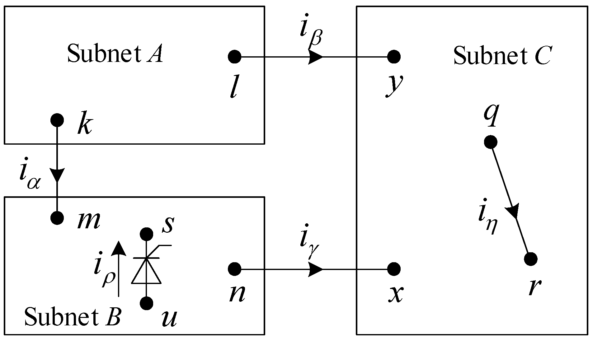
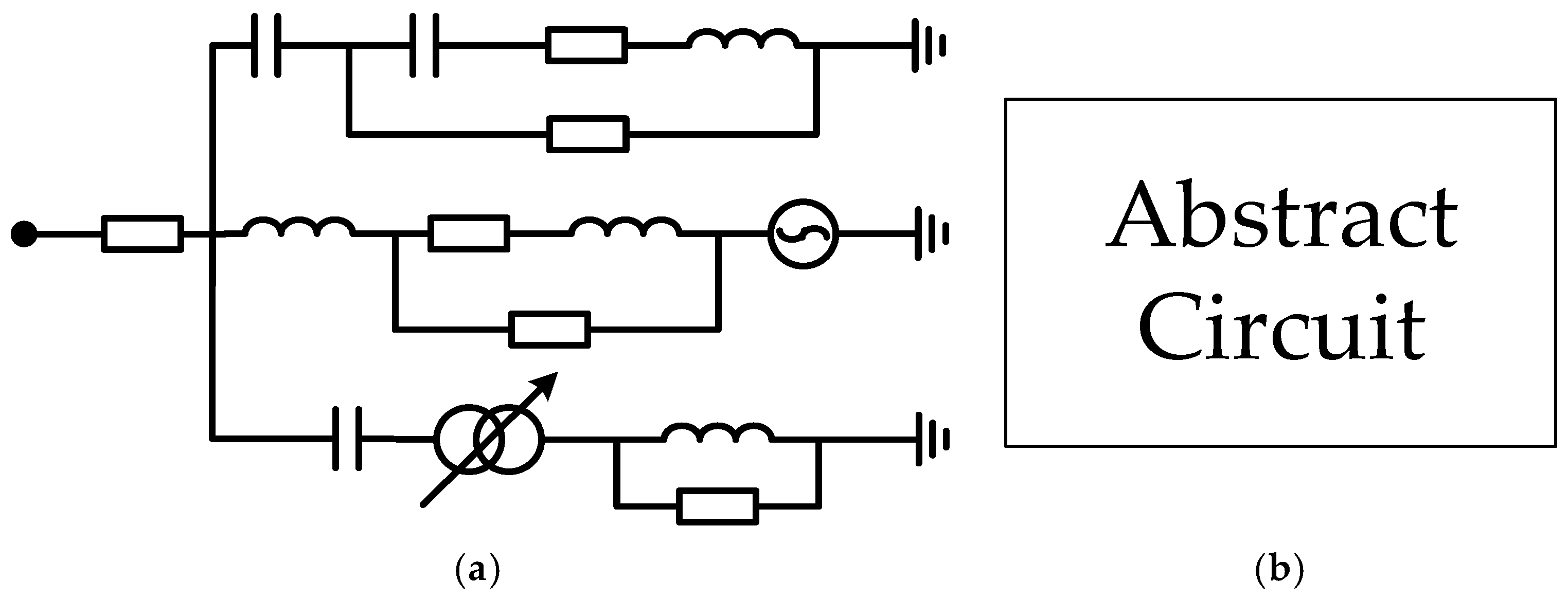
Taking an abstract AC/DC hybrid power system as an example, the parallel algorithm considering nonlinear characteristics of the power system is described. The partition of the sample power system is shown in
Figure 1. Subnet B is a DC grid, including rectifiers, inverters, DC lines; the components in branch set
s-u are switches, so the admittance matrix of subnet
B is changing. Both subnet
A and
C are AC grids, and supposing the component parameters of subnet
A are unchanging, which is changing in branch set
q-r of subnet
C under different operation states (such as an on-load tap changer, OLTC), the admittance matrix of subnet
A is unchanging, which is opposite to that for subnet
C.
It is worth noting that the node in
Figure 1 does not specifically refer to a single node, but represents some node set, and we also suppose that “node set-node set” represents a branch set, such as
l-y. In these branch sets,
k-m,
l-y, and
n-x are used for network partitioning and are used to divide the network into different parts.
s-u and
q-r are the branch set with changing parameters, and they do not participate in the formation of admittance matrices.
The corresponding nodal equations of each subnet are as follows [
6]:
where
Gi,
Vi, and
hi denote the admittance matrix, node voltage, and accumulated current of subnet
i (
i denotes
A,
B, and
C), separately. In particular, the elements of
GB and
GC don’t include
s-u and
q-r parameters, respectively. Therefore,
GA,
GB, and
GC are constant matrices.
iα,
iβ, and
iγ denote the links’ current between subnets.
iρ and
iη denote the links’ current of
s-u and
q-r.
pk,
pl,
pm,
pn,
py,
px,
pq,
pr, and
pu denote connectivity arrays, which reflect the relationship between the nodes and links’ current. In particular, let
pη denote
pq +
pr,
pρ denote
ps +
pu.
As for
s-u and
q-r, the branch equations are:
where
zρ,
zη, and
eρ,
eη denote branch links’ Thevenin impedances and Thevenin voltages of
s-u and
q-r, separately.
From Equations (4) and (5), the dimension of iρ and iη are proportional to the number of changing branches. In general, the number of these changing branches in the AC subnet is small and is uncertain for the DC subnet. For example, changing branches of twelve pulse rectifier circuits is much less than modular multilevel converter (MMC). As for the proposed method, the number of changing branches should not be too large, or the calculation amount of the links’ current would be extremely large.
As for
k-m,
l-y, and
n-x, the branch equations are [
6]:
where
zα,
zβ,
zγ, and
eα,
eβ,
eγ denote the branch links’ Thevenin impedances and Thevenin voltagse of
k-m,
l-y, and
n-x, separately.
By combining Equations (1)–(8), Equation (9) can be obtained:
iα,
iβ,
iγ,
iρ, and
iη could be obtained by solving Equation (9), and
VA,
VB, and
VC could be solved via putting them into Equations (1)–(3). From Equation (9), solving the inversion of the admittance matrix is inevitable when obtaining the links’ current. From above,
GA,
GB, and
GC are constant matrices, and their inversion is needed to be solved once during the entire simulation. Additionally, both links’ current of the changing and partition branches are solved together, which is different from the literature [
7]. In [
7], changing branches are dealt with in their subnet calculation unit.
2.2. Physical Significance of the Parallel Algorithm
In the electromagnetic transient parallel algorithm based on MATE, the power system is divided into several subnets. The influences among different subnets are reflected through the links’ current obtained by the Thevenin equivalent. The Thevenin equivalent regards some nodes as the research object, and acquires equivalent parameters in view of these nodes. Taking node k and l of subnet A as an example, the Thevenin voltage and impedance are described as follows:
In Equation (9), and denote the Thevenin voltages of nodes k and l, respectively. and denote the Thevenin self-impedance of nodes k and l, respectively. and denote the Thevenin mutual-impedance between node k and l.
4. Simulation Process
In this section, the optimization of the algorithm is described. Then the simulation flowchart is shown to describe the simulation procedure.
4.1. Optimization of Simulation Process
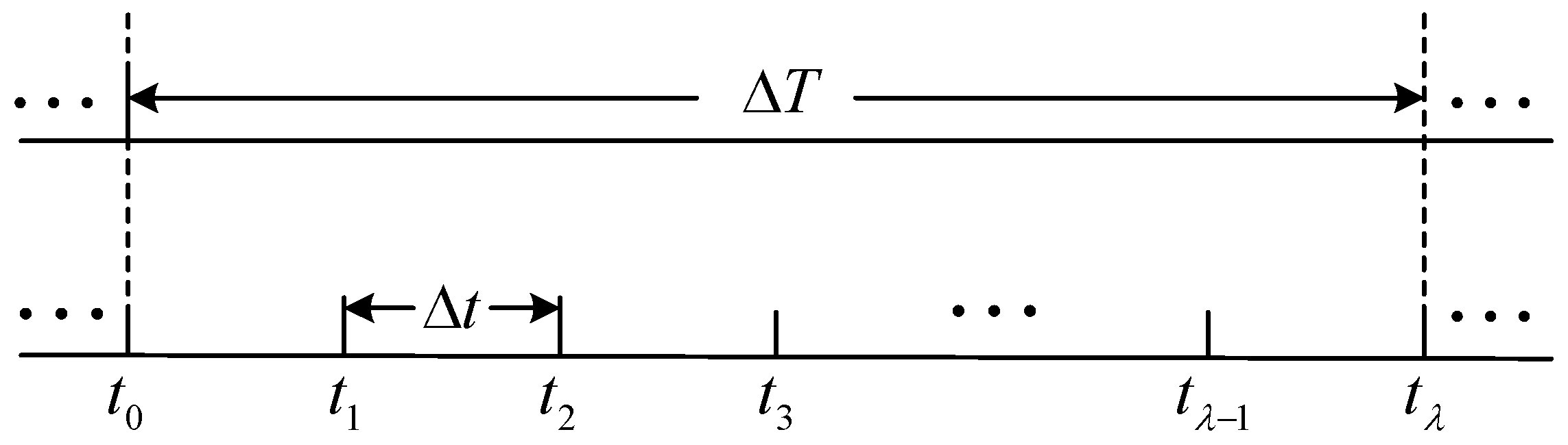
The components in Equation (17) include the network solution in non-synchronized and synchronized time among the last . The summation part of the history term in Equation (17) could be updated at the end of each small time step , which avoids a large amount of calculation if all the addition tasks are executed when all the non-synchronized solutions have been obtained.
In addition, the process of calculating
VA,
VB and
VC is optimized. The Equations (1)–(3) are simply deformed and written in matrix form, and they are shown as follows:
The first term on the right side of the Equation (18), could be calculated before the links’ current are obtained (i denote A, B, and C). Therefore, parallel calculations are used for solving and the links’ current. When the links’ current are solved, we substitute them into the second term on the right side of the Equation (18), and VA, VB, and VC can be solved.
4.2. Simulation Process
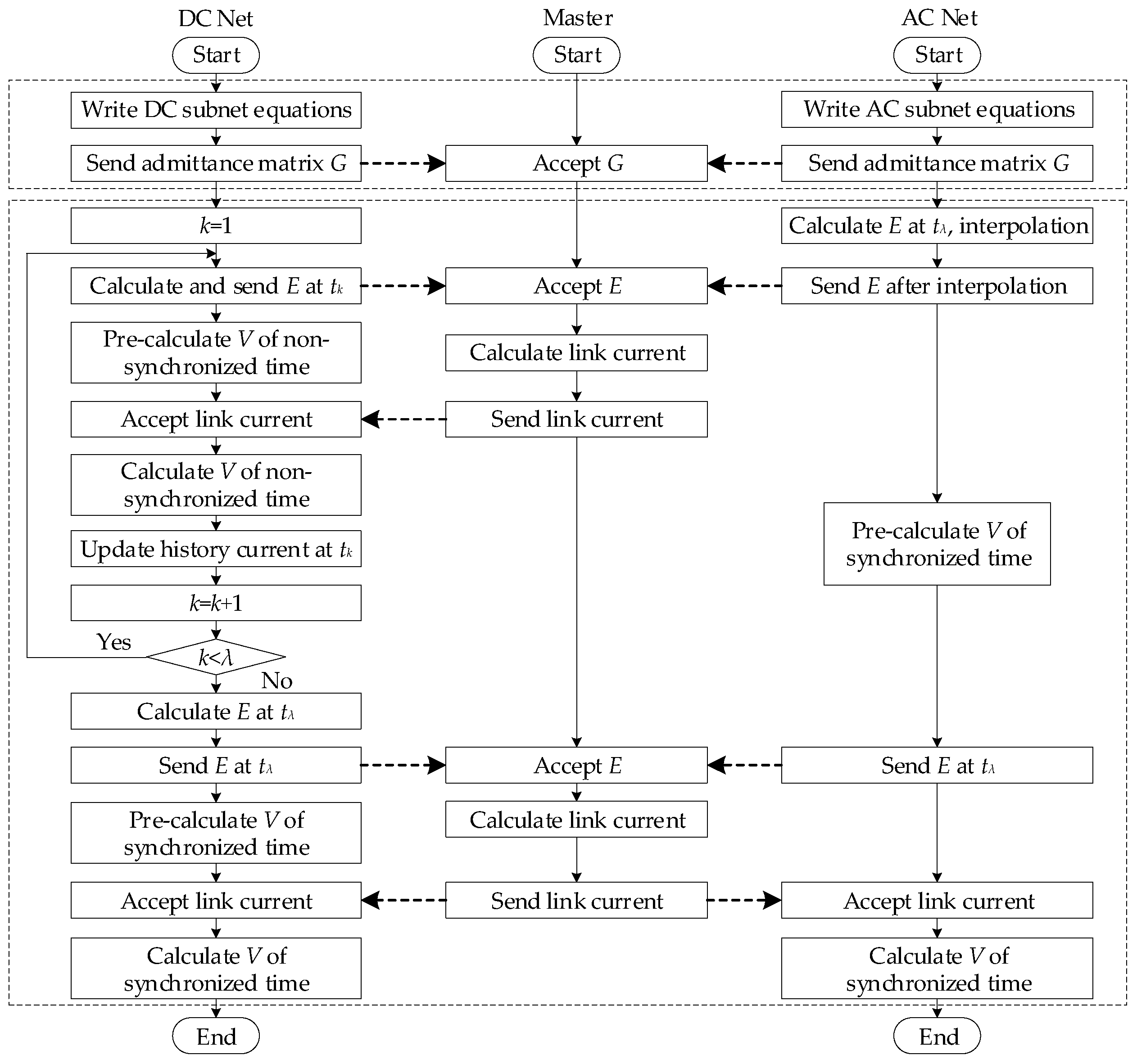
Figure 3 is the simulation process chart of this algorithm. The upper dashed box is the preprocess, which is mainly used for obtaining the admittance matrix and its inversion, and only needs to be calculated once in the whole simulation process. The lower dashed box is a simulation process among
, which is mainly used for pre-solution of the subnet network equation, acquiring the connection line current and the calculation of the node voltage. The calculation process of other
is exactly the same as the lower dashed box.
In the upper dashed box, network equations of the DC and AC nets need to be written, and their admittance matrices are sent to the master side before simulation. Supposing the network has been solved before t0, the calculation process of the lower dashed box is illustrated as follows:
- (1)
For the AC subnet, calculate and based on the calculation results of t0, which is shown in Equations (10) and (11), and interpolate to obtain their interpolation Thevenin voltage, which is shown in Equation (12).
- (2)
For the DC subnet, let k = 1.
- (3)
For the DC subnet, calculate based on the calculation results of .
- (4)
Send , , and to the master side, calculate the link currents according to Equation (9) and send them back to the DC net.
- (5)
During procedure (4), is calculated at the same time.
- (6)
VB is calculated according to the second line of Equation (18), and is updated.
- (7)
Let k = k + 1, and judge whether k < λ.
- (8)
If k < λ, return to procedure (3). If not, go to procedure (9).
- (9)
For the DC subnet, calculate based on the calculation results of the whole .
- (10)
During procedures (4) to (9), and are calculated at the same time, and , could be obtained.
- (11)
Send , and to master side, calculate link currents according to Equation (9) and send them back to the AC and DC nets.
- (12)
During procedure (11), is calculated at the same time.
- (13)
VA, VB, and VC are calculated according to Equation (18).


