4.1. Calculation Model for Corona Onset Voltage Considering the Outer Strand of the Conductors
As the AC corona discharge has a polar effect, the conductors’ negative polarity corona discharge precedes positive polarity corona discharge, so the negative corona discharge model was used here. The negative corona discharge model has been described in detail in references [
21,
22,
23,
24,
25]; therefore, in this paper, only the sections of the model that have been improved are discussed:
In high-altitude areas, the corona onset characteristic is mainly influenced by the collision ionisation coefficient α and the electron attachment coefficient η at different atmospheric pressures; eventually the ionised boundary surface (α(r) = η(r)) was changed, where r is the distance between the ionised boundary and the conductor.
The parameters of
α and
η are functions of
E (the electric field strength, kV/cm) and
p (the air pressure, kPa). The collision ionisation coefficient
α and the electron attachment coefficient
η are given, for different ranges of
E/
p, in reference [
23]. In the experiments, the temperature changed within the range from 12.8 to 14.3 °C (the difference is less than 1.5 °C), therefore, the influence of temperature can be ignored in the analysis of the experimental results. The parameters
α and
η, considering relative humidity, are also given in reference [
25].
The air pressure
p can be transformed by the relationship between altitude and air pressure is:
where
H is the altitude (km), in this paper,
H = 2.2 km,
p0 represents the standard atmospheric pressure (101.325 kPa), and
k = 10.7 [
20].
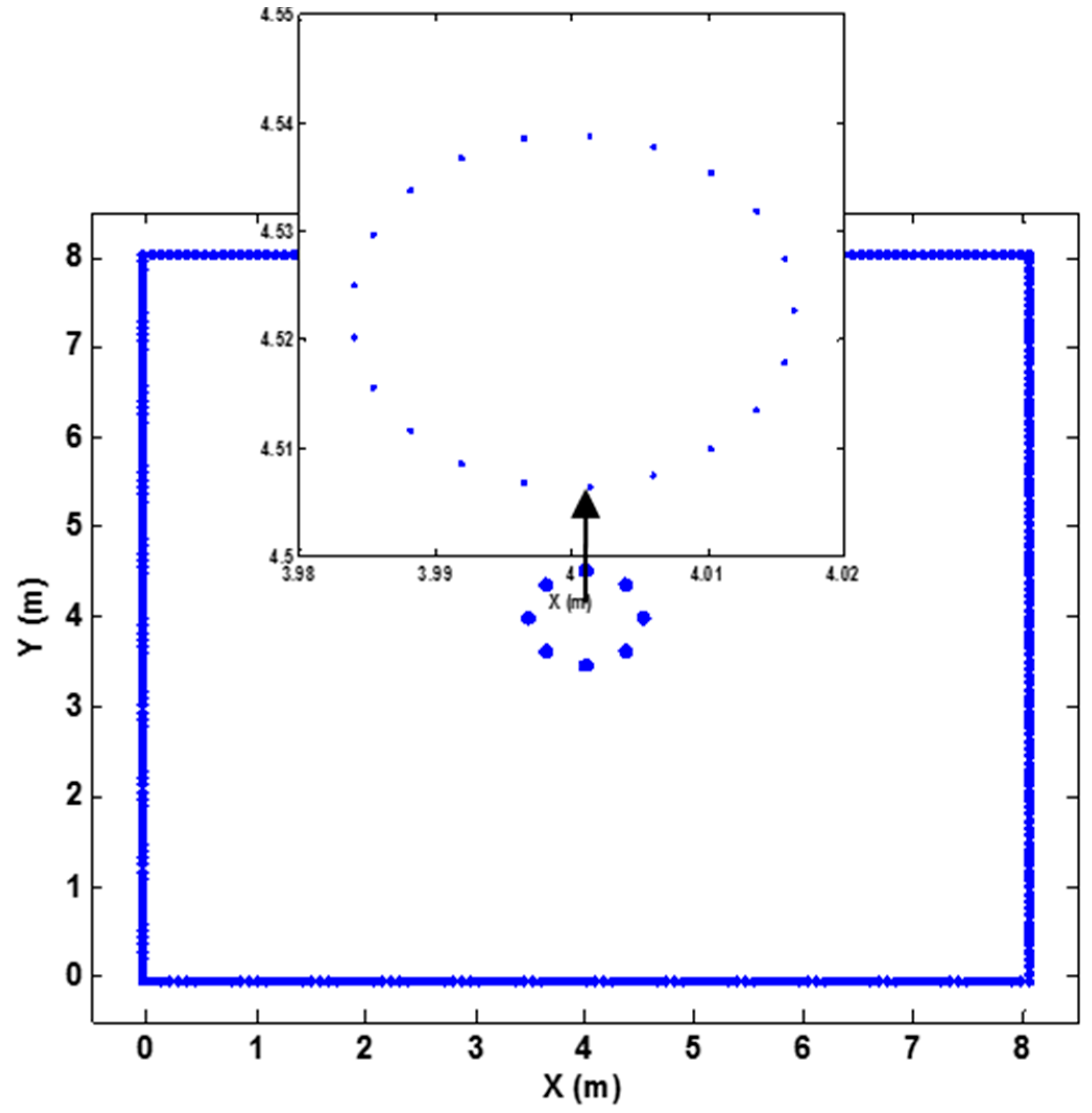
The former study assumed that stranded conductors have a smooth cylindrical structure, ignoring the influence of outer strands on the electric field E and the geometric factor g(r) in the model.
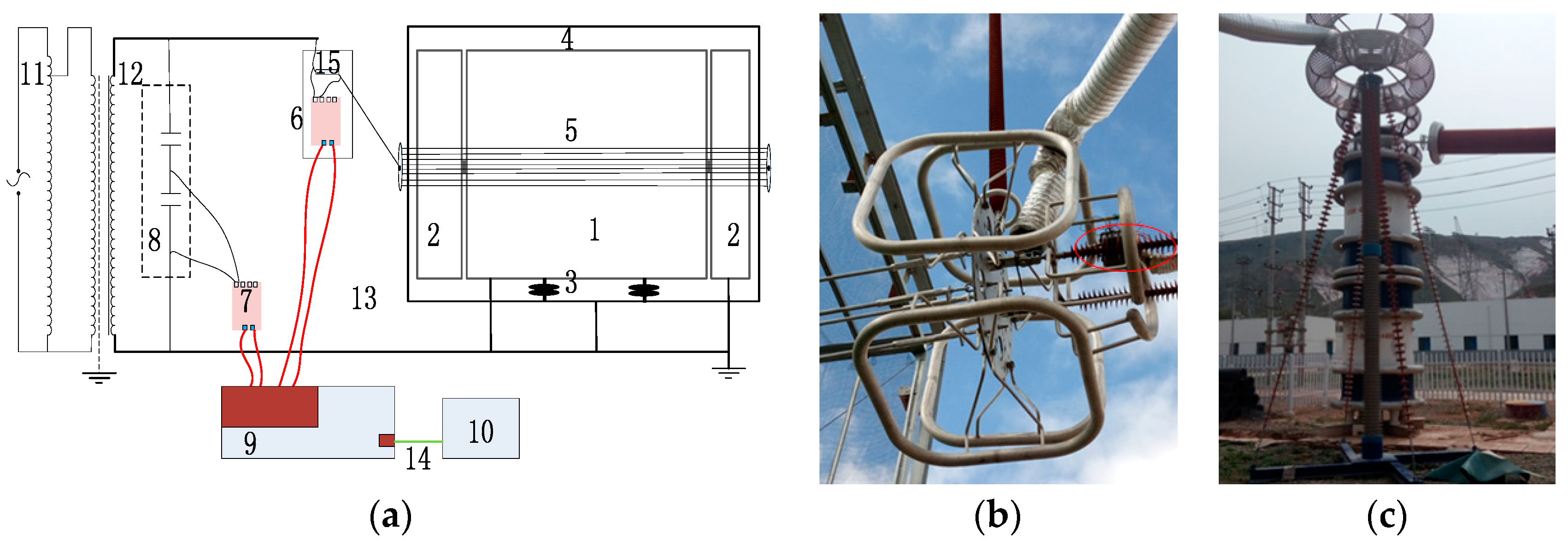
In this paper, the authors calculated the electric field strength
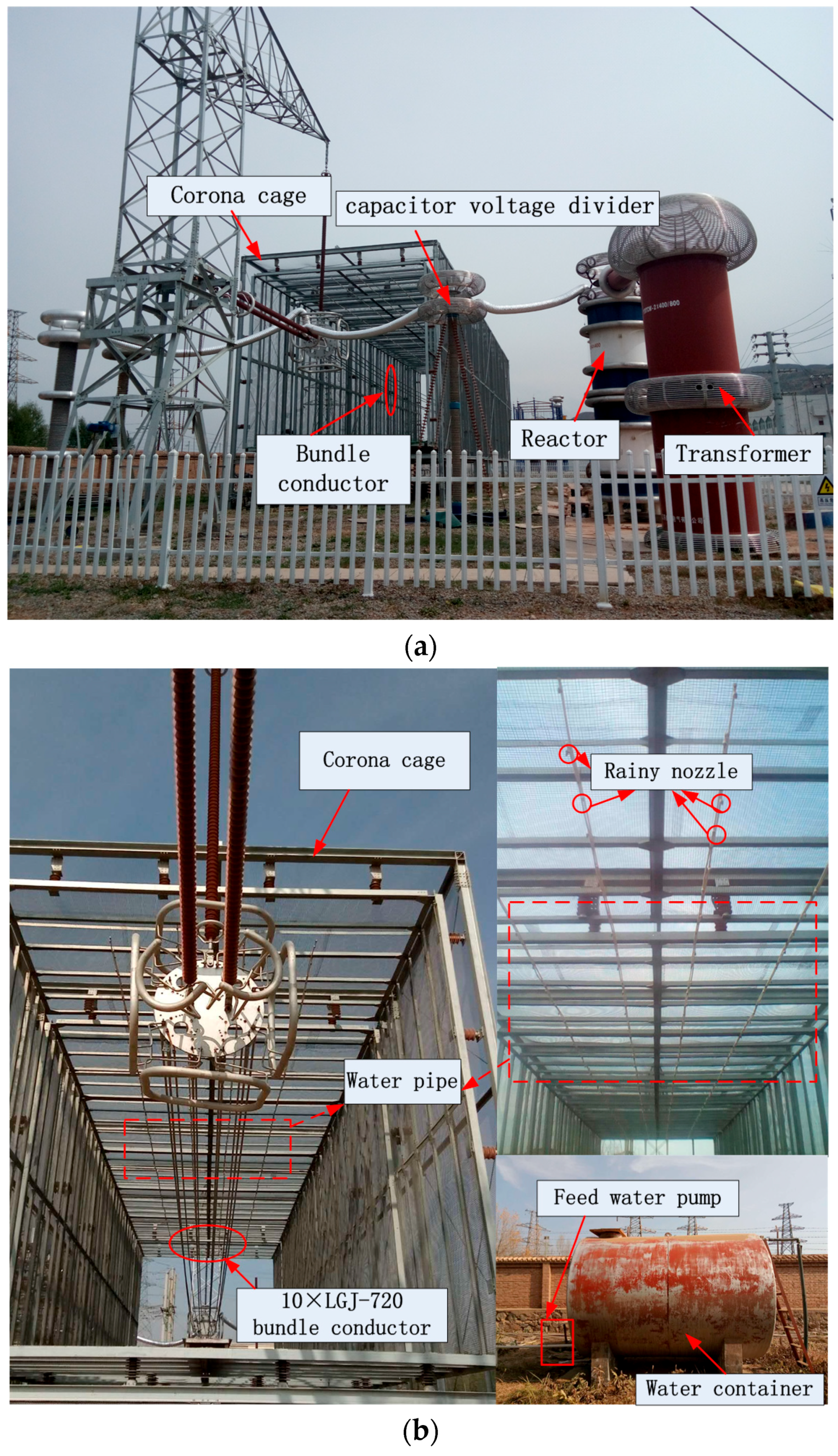
E around the bundle conductors considering the outer strands based on the charge simulation method, as shown in
Figure 6.
Assuming that the voltage applied to the conductor was
Ut, then:
where
Qcond is the simulated charge on the conductor;
Qcage is the simulated charge on the walls of the corona cage;
Pcond1 and
Pcond2 are the potential coefficients of
Qcond at the charge-emitting points on the conductor surfaces and charge-matching points on the corona cage walls;
Pcage1 and
Pcage2 are the potential coefficients of
Qcage at the charge-emitting points on the conductor surfaces and charge-matching points on the corona cage walls. fx_cond and fy_cond denote the field intensity coefficients of
Qcond in the
X- and
Y-directions at any point in the field,
fx_cage and
fy_cage are the field intensity coefficients of
Qcage in the
X- and
Y-directions at any point in the field.
Qcond and
Qcage can be obtained by solving Formulae (3) and (4) simultaneously, and then the electric field distribution at any point in the field can be obtained from Formulae (5) and (6) based on the superposition principle:
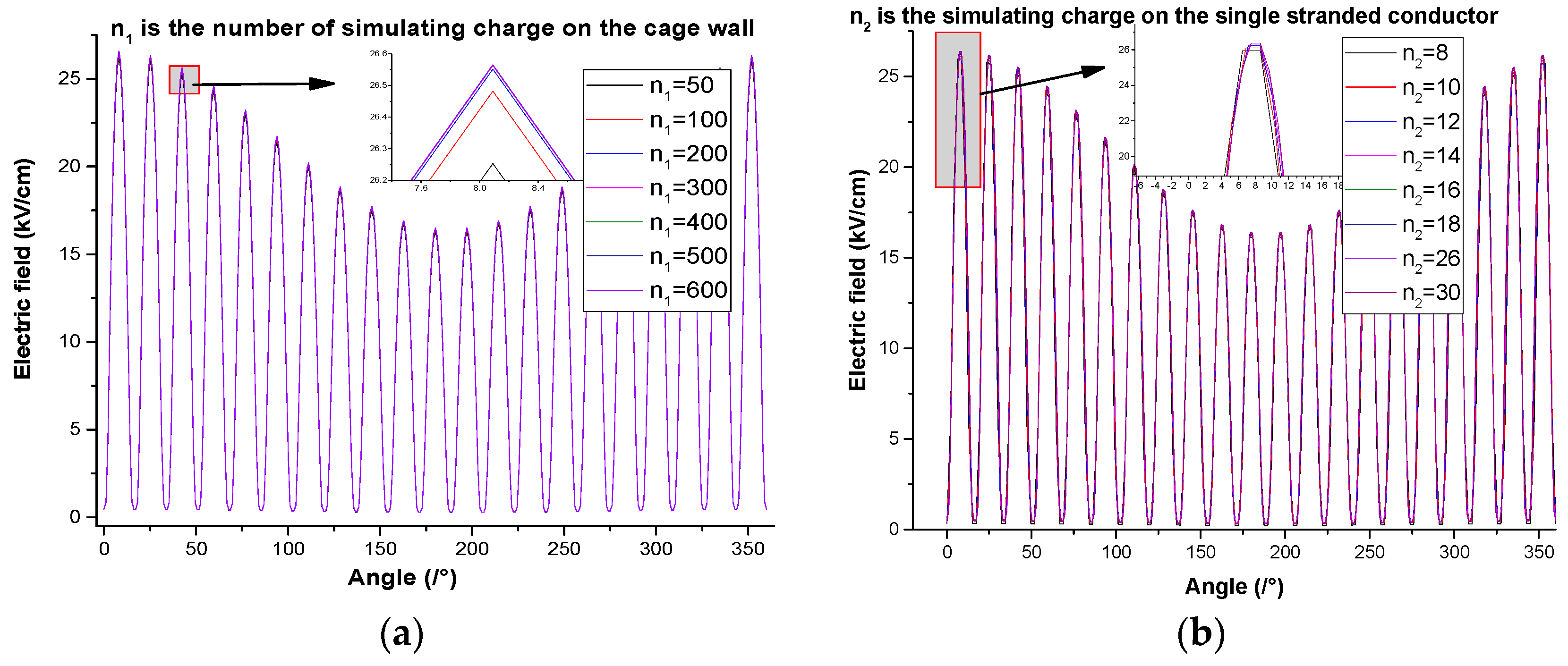
Figure 7a illustrates the electric fields on the walls of the corona cage calculated using different simulated charges, the computation error of the electric field between two adjacent calculation results is shown in
Table 6; when the number of simulated charges on the corona cage exceeds 300, the electric field intensity of the stranded conductor remains unchanged.
Figure 7b shows the calculated electric field distribution on the surface of the stranded conductor calculated by using different charges on each strand, the computation error of electric field between two adjacent calculation results is shown in
Table 7; when the number of charges on a single strand exceeds 14, the calculated electric field on the strand surface remains unchanged. Therefore, 17 simulated charges were applied to each strand of the outer strands of sub-conductors for these simulations, and 400 simulated charges were applied to the corona cage wall. In this way, the electric field on the surface of the stranded conductor was determined.
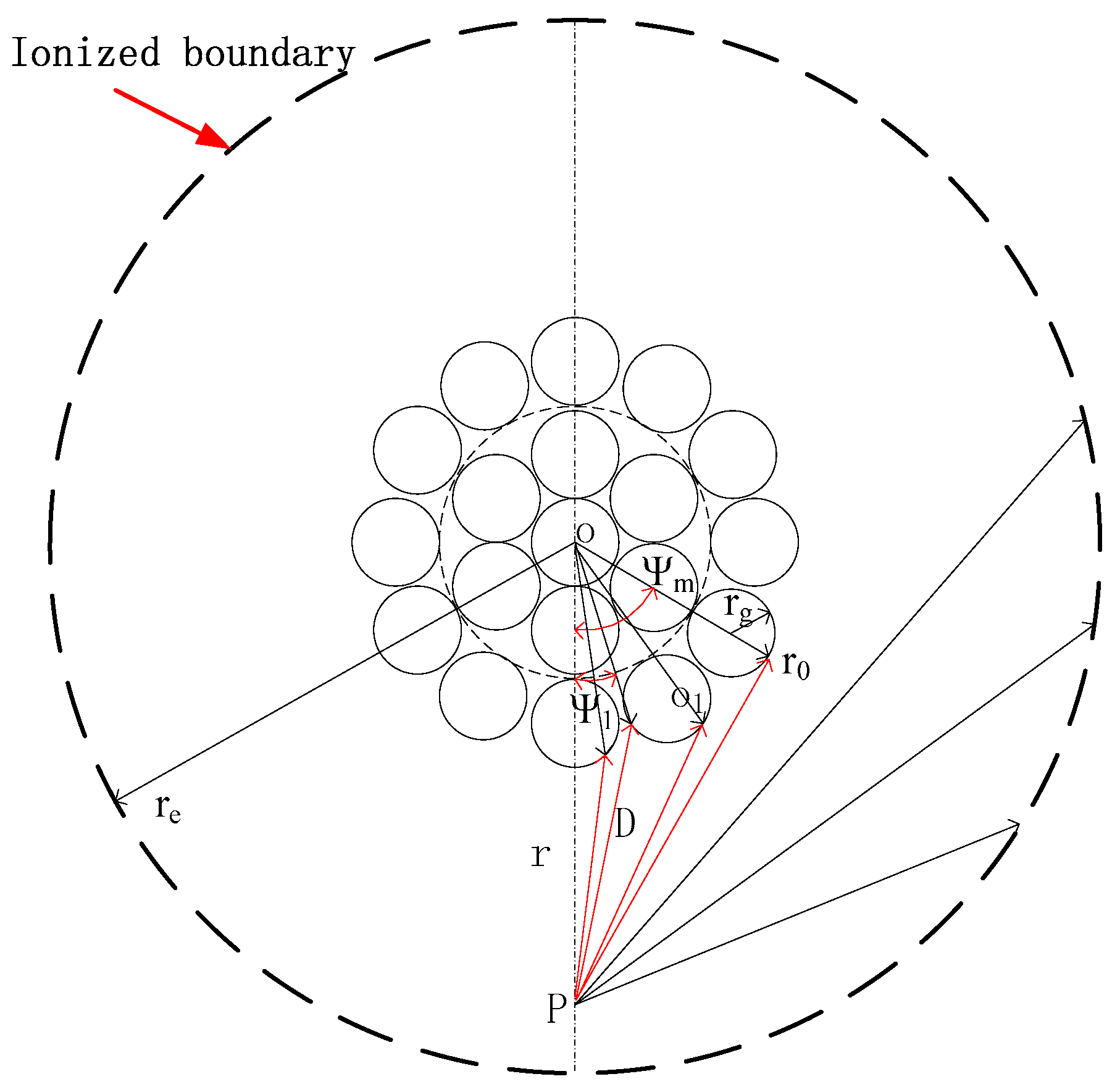
For the stranded conductor, the geometric factor
g(
r) can also be decomposed into the product of the radial component
grad(
r) and the axial component
gaxial(
r). The axial component
gaxial(
r) is the same as that of the smooth conductor, but the radial component
grad(
r) is different, as shown in Formula (8). Photon emission in the radial direction in the ionised zone is shown in
Figure 8.
In the formula,
where,
rg the radius of the outer strand,
n is the number of strands in the outer layer.
4.3. Equivalent Roughness Coefficient of Bundled Conductors
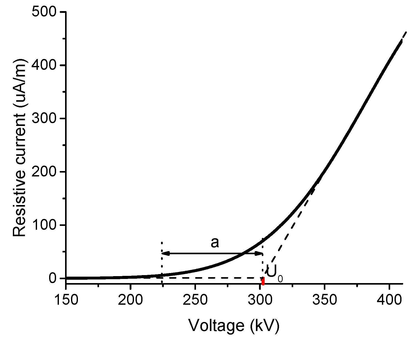
The equivalent roughness coefficient of the conductor,
m, is defined by:
where,
Uincc is the corona onset voltage of the stranded conductor, kV; and
Uincs is the corona onset voltage of ideal conductors having the same outer diameter as the stranded conductor, kV.
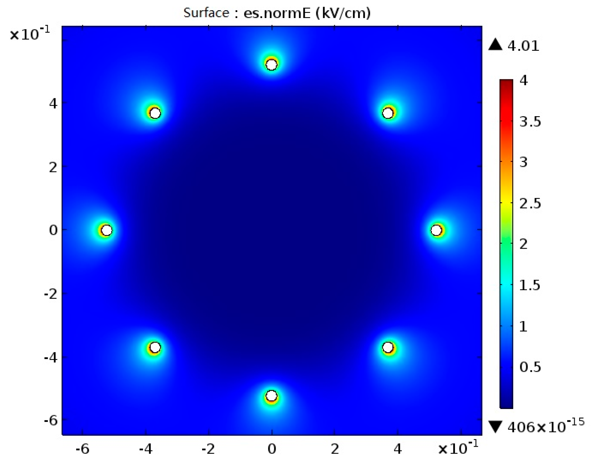
For the 6 × LGJ720, 8 × LGJ720, 10 × LGJ720 and 8 × LGJ630 bundled conductors, due to the number of outer stands being 21, 21 simulation charges were evenly arranged on the periphery of the circle with the same radius of each sub-conductor to simulate the electric field around an ideal smooth conductor, as seen in
Figure 9. The comparison of the conductor surface electric fields between ideal smooth cylindrical conductors and stranded conductors is shown in
Figure 10.
The corona onset voltage of the ideal smooth conductor with the same radius and bundle type (roughness coefficient
m = 1) is calculated for an altitude of 2200 m above sea level. In addition, the surface roughness coefficients for the four different weather conditions were calculated (
Table 9), whereby the roughness coefficient of the wet conductor and that under rainy conditions was the ratio of the tested corona onset voltage to the calculated corona onset voltage of the ideal smooth conductor under the dry weather conditions. It can be seen from
Table 6 that, for the LGJ720 bundled conductor, the roughness coefficient shows a decreasing trend with increasing numbers of bundles under the same meteorological conditions.
For wet conductors, or under rainy conditions, there are suspended, or fixed, water droplets on the conductor surface. The presence of water droplets changes the surface state and reduces the equivalent roughness coefficient of a conductor. Due to the joint effects of gravity, adhesion, surface tension, and the electric field force, water droplets will be deformed and vibrate at a frequency of twice that of the electric field frequency [
26]; near the peak AC voltage, water droplets are flattened, while near the zero-crossing point of the voltage, they become conical and finally drop, forming smaller droplets, which are ejected to surrounding areas.
The roughness of the wet conductor lies between that of the dry conductor and the conductor under rainy conditions. This can be explained as follows: the conductor surface gradually dries, owing to the “Asakawa effect” with longer application of voltage under wet conductor conditions, and the number of water droplets on the conductor surface decreases such that the surface irregularities are reduced and the roughness is increased, but remains smaller than that in a dry conductor. Under rainy conditions, the roughness coefficient of the conductor decreases with increasing rainfall intensity and tends to reach saturation. The number of water droplets on the conductor surface increases with rising rainfall intensity at low rainfall intensities, which alters the electric field on the conductor surface and reduces the corona onset voltage. With further increases in rainfall intensity, the surface tends to reach saturation, and the continuously increasing rainfall intensity plays a limited role in reducing the roughness coefficient, as the water droplets are quickly replaced after falling.


